Abstract
Wildlife–vehicle collisions (WVCs) remain a significant cause of animal mortality worldwide, particularly in regions experiencing rapid road network expansion. During the COVID-19 pandemic, a number of studies reported decreased WVC rates, attributing this trend to reduced traffic volumes. However, the validity of the simplified assumption that “fewer vehicles means fewer collisions” remains underexplored from a mechanistic perspective. This study aims to reevaluate that assumption using two simulation-based models that incorporate both the physics of vehicle movement and behavioral parameters of road-crossing animals. Employing an inverse modeling approach with quasi-realistic traffic scenarios, we quantify how vehicle speed, spacing, and animal hesitation affect collision likelihood. The results indicate that approximately 10% of modeled cases contradict the prevailing assumption, with collision risk peaking at intermediate traffic densities. These findings challenge common interpretations of WVC dynamics and underscore the need for more refined, behaviorally informed mitigation strategies. We suggest that integrating such approaches into road planning and conservation policy—particularly under the European Union’s ‘Vision Zero’ framework—could help reduce wildlife mortality more effectively in future scenarios, including potential pandemics or mobility disruptions.
1. Introduction
Wildlife–vehicle collisions (WVCs) represent a major conservation and safety challenge across the globe. In Europe alone, an estimated 194 million birds and 29 million mammals are killed annually on roads [1], with ungulates accounting for over one million deaths each year [2,3]—a mortality scale comparable to that caused by legal hunting. These figures underscore the magnitude of road networks as ecological filters and drivers of population decline.
While the societal and ecological costs of road mortality are well documented, metaphors have occasionally been used to describe its devastating impact. One such example is the expression “Moloch of the asphalt,” which dates back to early 20th-century American journalism. Originally referring to an ancient deity of the Ammonite and Canaanite-Levant civilizations associated with child sacrifice, “Moloch” became a metaphor for the destructive power of automobiles and urbanization [4]. Though evocative, such analogies are best viewed as rhetorical devices illustrating the perceived brutality of modern traffic systems, particularly given the high volume of animal deaths [5,6].
Against this backdrop, the COVID-19 pandemic provided a unique, unintended experiment: a large-scale reduction in human mobility, often referred to as the Anthropause [7]. This global pause in travel and economic activity led to various ecological responses, one of the most frequently cited being a decrease in wildlife–vehicle collision(s) (WVCs). This observation forms a central part of the Anthropause argument [7]. The Anthropause revolves around a significant global reduction in modern human activities, particularly travel, and explores how we can share space with wildlife on our crowded planet [8]. The WVC decrease phenomenon is primarily attributed to a reduced traffic load, which can be measured through metrics such as lower traffic congestion, fewer vehicles on the roads, and a decrease in vehicle kilometers traveled [7,9,10,11,12,13,14]. This interpretation is frequently summarized by the assumption that “fewer vehicles leads to fewer WVCs,” a premise that underlies much of the Anthropause-related WVC literature.
While the assumption that reduced traffic universally leads to fewer WVCs remains widespread, the recent literature urges caution, as the monitoring strategies employed across WVC studies vary considerably, introducing potential sources of heterogeneity in reported outcomes. These methodological differences span the geographic context (e.g., urban vs. rural settings) [15,16], the temporal resolution and duration of monitoring [17], the degree of reliance on citizen science data [18,19,20,21,22,23], and the characteristics of the road network examined—ranging from ones a few hundred meters in size to major highways [23,24,25]. While reported animal mortality rates vary across studies, species, and environmental setups, a general trend appears to be quasi-universally accepted: lower instances of WVCs are associated with reduced traffic pressures.
Despite the prevalence of this assumption, a closer examination of the emerging literature reveals a more nuanced picture. During the early months of the pandemic, when strict lockdown measures dramatically altered human mobility patterns, several studies attempted to quantify changes in WVCs across diverse ecological and geographic contexts. A targeted search in Web of Science using search strings combining ‘COVID OR pandemic,’ ‘lockdown’, ‘animal *’, “wildlife-vehicle collision *” OR “animal road kill *” identified relevant research from more than 20 countries or regional setups. These studies were highly heterogeneous in design, yet their findings could be broadly classified into three outcome categories: (1) a decrease in WVCs, (2) an increase in WVCs, and (3) no effect. Each publication contributes to the overall percentage of categories. This classification scheme supports a bottom-up approach in ecological research, which is widely utilized in the literature on the Anthropause [7]. Although the first category dominates, roughly 20% of studies reported no effect, and 10% documented an unexpected increase in roadkill despite reduced traffic volumes [15,26,27,28,29,30]. This heterogeneity challenges the assumption of a universal traffic–road mortality relationship, suggesting that additional ecological, behavioral, and environmental variables may mediate the effect of traffic reductions on wildlife road mortality.
Building on this observed heterogeneity, a deeper examination reveals that a notable twofold paradox emerges. First, a non-negligible number of cases indicate that lockdown-related traffic conditions had little or no significant impact on animal road mortality, and in some cases, WVCs even increased. Interestingly, among the cases analyzed, most ‘no effect’ and ‘increased WVC’ results were reported as exceptions or deviations in studies that involved multiple setups or comparisons across different species [15,26,27,28,29,30]. This pattern suggests that the outcomes of traffic changes are not uniformly predictable and are likely influenced by species-specific biological, ecological, behavioral, and phenological traits. These traits, together with collision dynamics shaped by car movements, driver behavior, road characteristics, and environmental factors, likely contribute to the observed heterogeneity. At its core, the incumbent generalization appears to rest on three fragile assumptions: (1) epistemically, a circular argument suggesting that “less traffic ‘equates’ to fewer road casualties”; (2) the notion that conflicting outcomes across taxa and contexts are mere exceptions; and (3) comparability across inconsistent metrics related to species richness, road types, and traffic proxies.
The second paradox stems from an equally striking observation: a significant rise in human–vehicle collisions (HVCs) during the same lockdown periods. Despite widespread mobility restrictions and reduced traffic volumes, pedestrians and cyclists fatalities did not decrease as expected—in several countries, they even increased [31]. National reports confirm that the UK recorded a 46% increase in HVC incidents during the lockdown, the USA 22.5%, Australia 4.4%, and Malaysia 8% [32,33]. Comparable patterns were noted in Italy, Germany, Greece, India, and Turkey, based on governmental statistics and independent communications. Although measurement methodologies varied, a consistent trend emerges: HVC levels remained high or even rose during the Anthropause. This pattern was likely exacerbated by increased cycling, reduced police presence, higher driving speeds, and persistent deficits in pedestrian and cyclist infrastructure.
This divergence between WVC and HVC trends fundamentally challenges the assumed linearity of the traffic–mortality relationship. It invites a reexamination of alternative dynamics, such as the nonlinear relationship between traffic density and vehicle speed observed in traffic theory [34,35]. Notably, Stiles et al. [36] proposed that lower traffic volumes can paradoxically increase crash risk by facilitating higher vehicular speeds—suggesting that reduced congestion does not necessarily equate to safer roads for either humans or wildlife.
Importantly, similar complexity is evident in the pre-pandemic WVC literature. While certain variables—such as proximity to natural habitats, gentle topography, road width, and seasonality—have shown consistent associations with elevated wildlife mortality risk [37], others—most notably traffic volume, road infrastructure type, and distance to urban centers—have demonstrated context-dependent and sometimes contradictory effects. Rather than serving as universally predictive variables, these factors have often been used post hoc to delineate WVC hotspots—localized areas with disproportionately high roadkill incidence [38,39,40,41]. This retrospective emphasis underscores a broader limitation: the field has largely relied on observational data without predictive modeling frameworks capable of integrating ecological, behavioral, and traffic-related variables.
In this study, we examine the potential for such an alternative generalization by developing and comparing two simplified but conceptually distinct models of WVC likelihood of a random WVC event. The first is a species-centered model, which posits that the likelihood of a WVC decreases exponentially based on the inverse of the frequency of an animal’s road crossings. The second is a horizontal interception model based on the mechanics of interception between two horizontally moving objects. It considers no vertical component, no acceleration, and constant velocity, time, and displacement range during their movement. This model examines how animals and vehicles interact on roadways, considering both parties’ movement patterns and the factors influencing the likelihood of collisions. Its approach resembles an agent-based model random walk simulation with drift, meaning consistent directional movement.
By comparing the outputs of these two models under normal and restricted traffic conditions, we aim to assess whether they yield divergent predictions and to identify the key parameters that influence the likelihood of WVCs. In carrying this out, we aim to develop a more generalizable and predictive framework—one that transcends post hoc interpretations and advances toward an explicitly mechanistic understanding of wildlife–vehicle collision risk. Based on this rationale, we hypothesize that reductions in traffic volume do not lead to a uniform decrease in WVCs. Instead, we propose that collision likelihood may follow a nonlinear response, with risk potentially increasing at intermediate traffic densities due to emergent interactions between vehicle spacing, speed, and animal road-crossing behavior.
2. Materials and Methods
The core epistemology of our methodology is defined as a blend of the two major schools of thought in ecology, which is necessary for addressing practical environmental problems. This includes the bottom-up approach, which accumulates empirical evidence from case studies and statistical patterns, versus the top-down approach, which generates general laws that then inform explanations for specific cases. We generate quasi-realistic data using various equations representing the physics of a WVC event. We supplement these equations with appropriate data from Monte Carlo simulations and conduct tests that simulate observations from real-world scenarios or controlled experiments (Figure 1).
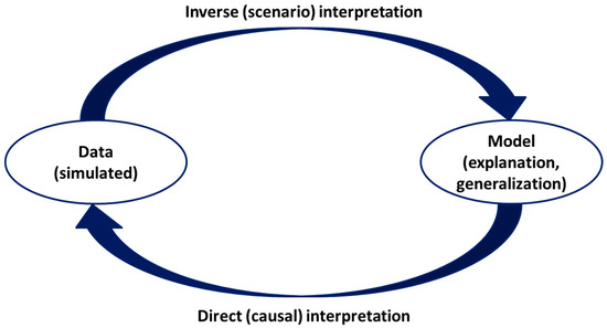
Figure 1.
A general scheme illustrates the rationale of the methodology of the approach we follow in this paper. The primary characteristic is that we employ an inverse model interpretation using simulated data to influence WVC events.
The modeling framework incorporates two conceptually distinct approaches. Model 1 is a species-centered behavioral model in which the likelihood of a wildlife–vehicle collision (WVC) decreases with reduced road-crossing frequency, following an exponential decay function. Model 2 applies a simplified ballistic formulation, conceptualizing WVCs as horizontal interception events governed by vehicle speed, inter-vehicle spacing, and animal movement rate. These models capture complementary aspects of WVC dynamics—exposure-driven versus mechanically driven risk—and allow comparative evaluation under normal and restricted traffic conditions.
To avoid repetition and establish clear simplifying assumptions in our two models, we will make the following distinction: we will not use the terms’ likelihood’ and ‘probability’ interchangeably. Since most published evidence on WVCs involves observed data, “likelihood” is a more appropriate approach for our study. Likelihood measures how plausible a parameter value is given the observed data. At the same time, probability refers to the likelihood of a specific event occurring and is calculated based on known parameters or conditions. This distinction is important because the outcomes of our models are based on simulated combinations of various variables, parameters, and coefficients related to animals, vehicles, and road conditions. Additionally, the differences in likelihood outcomes from the same model, when using different ranges of parameter values, can yield negative results, which is not possible for probabilities.
2.1. WVCs as a Simplified Horizontal Ballistics Problem
The collision of a vehicle with an animal or a pedestrian is generally not classified as a ballistic event. Ballistics focuses on the angle at which a projectile is launched, with its trajectory determined by horizontal and vertical motions. Notably, these two types of motion do not interact with each other. Then, the ‘ballistics’ of a WVC considers only the horizontal motion, and the launch angle φ is 0, meaning cos(φ) = 1. We consider forces such as friction or drag to be negligible in this case. For the definition of parameters, variables, or constants used hereafter, refer to Table 1.

Table 1.
Variables and factors of the vehicle–animal–motorway triptych that interfere with a wildlife–vehicle collision incident. The variables, constants, and equations used in our WVC ballistics problem are presented in bold.
A WVC incident occurs in a stretch of road after encountering a traveling vehicle with speed sv and a roaming animal crossing the motorway with speed sw (Figure 2). For both colliding subjects, at a point or stretch of the road, the distance traveled in intersecting trajectories equals the product of speed (sv or sw, respectively) by time. Heuristically, the likelihood of a ground-roaming animal colliding with a vehicle, denoted by k hereafter, could be estimated after the time it takes to cross the road of width π (and x lanes) and the time separation between vehicles.
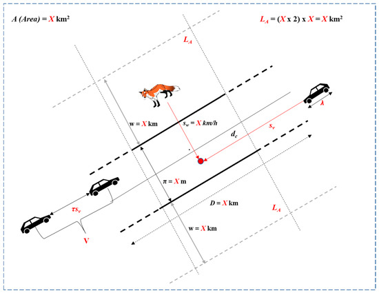
Figure 2.
A hypothetical WVC incident featuring a ground-roaming animal, the minimum variables, factors, and equations (X), and data necessary to examine it as a ballistics problem. Red symbols denote the analytical components of the model—variables, parameters, and expressions used in the equations (e.g., v, sv, A, La, and X)—as well as the collision point and the measured or derived distances. Black and gray graphics depict the scene (roadway, vehicles, animal), while gray dashed lines indicate lane or road boundaries, whose lengths are labeled in red to correspond to their respective variables.
The animal’s crossing time equals tw = π/sw (units converted accordingly, in km and h). A WVC will occur if the vehicle’s speed sv (and distance d from the crossing point, i.e., the time to reach the crossing point) is within a critical distance dc equivalent to the stretch of road of width π at the time the animal begins its crossing with a roaming speed of sw. The time to transport N vehicles over a critical distance is as follows:
dc = sv × tw = (sv/sw) × π
In a general form, the probability that an animal crosses the road n times and then gets run over during its n + 1st attempt is as follows:
p = k × (1 − k) n
Using general population and behavior data for an animal, a valid approximation of this probability might be expressed as follows:
p = n × k
Equivalently, this probability per unit time is given by the following:
where WVCr is the rate of roadkill incidents (e.g., individuals per day) and R is the population at risk in the road vicinity.
p = WVCr/R
Another heuristic calculation for the crossing frequency n can be deduced indirectly as follows:
where w is the average location distance of the animal to the road, in km; sw is the mean roaming speed of the animal, in km/day; and ρ is the ratio of animal roaming time/day. Combining the expressions mentioned above, we arrive at the following heuristic equations: the size of the population at risk is as follows:
n = (ρ × sw)/w
R = WVCr/n × k
And an alternative estimation of the collision likelihood k of a WVC is as follows:
where Iv is the average inter-vehicle spacing (km). This formulation ensures that k remains a dimensionless ratio, as it is derived from the quotient of two distances and scaled by the inverse of animal speed.
k ≈ (dc/Iv) × (1/sw)
Table 1 summarizes and defines the variables and factors related to vehicles, motorways, and wildlife influencing the probability of a WVC. Equations (1)–(7) represent a system used to determine k, which corresponds to the likelihood of a WVC event. This approach is advantageous as it reduces the number of parameters, constants, and even equations from Table 1 that require specific measurements, which can introduce significant uncertainty in accurately solving the ballistics problem. For instance, variable/factor V8, in Table 1, represents the congestion factor. By definition, the congestion factor is influenced by traffic restriction measures and typically represents the ratio of actual traffic volume to the road’s maximum capacity. One variable that affects the congestion factor is V6, where V = τ × sv, with τ representing the driver’s reaction time to a potential hazard, such as an animal or a person crossing the road. The average reaction time of a driver when responding to a road obstacle can vary based on several factors, including the driver’s alertness, experience, and the time of day. Here are some general findings regarding reaction times: (1) daylight reaction time is approximately 1.5 s; (2) nighttime reaction time is approximately 2.5 s; and (3) the general average reaction time is around 0.75 to 1 s. These durations indicate the time it takes for a driver to perceive an obstacle and initiate a response, such as moving their foot from the accelerator to the brake pedal. Variability in the parameter τ, which ranges from 0.75 to 2 s, creates significant uncertainty in the accuracy of predictions for any equations of interest, especially the congestion factor.
2.2. Exploration of Equations as a System of the Ballistics Problem
The derived equations reveal that factors influenced by COVID-19 confinement measures, such as human mobility and travel restrictions, do not directly affect the likelihood k of a WVC incident nor the size of the population at risk R. Instead, they aim to identify the determinants of traffic volume that are affected by human confinement or reduced mobility measures. Additionally, vehicle speed and congestion, along with vehicle fleet composition, λ, can either increase or decrease the likelihood of road mortality. This analytical framework enables us to test whether traffic volume reductions due to lockdowns lead to proportionally lower WVC rates, or whether other traffic dynamics, such as changes in speed and spacing between vehicles, introduce nonlinear or unexpected effects.
Since the likelihood k of a WVC event is expressed in Equations (2), (3) and (7), the following simulation models are developed to examine their behavior under different assumptions.
- Model 1—The exponential decay version:
Deducing an approximation of k from Equation (2), we obtain the following:
p = k × (1 − k)n
Assuming that k << 1, algebraic manipulations allow us to demonstrate that (1 − k)n≈ e−1 ⇔ k ≈ 1 − e(−1/n). This formula can be written alternatively as k ≈ 1 − e(−w/ρ.sv), using Equation (5) for n, if data on an animal’s roaming behavior is available and accurate (Appendix A).
- Model 2—The horizontal ballistic version:
Deducing an approximation of k from Equation (7), we obtain the following:
k ≈ (dc/Iv) × (1/sw)
This equation relates k to dc, Iv, and sw. It suggests that k is proportional to the ratio of dc to Iv, scaled by 1/sw. The definitions of the critical distance dc, the average interval between vehicles Iv, and the roaming animal mean daily speed sw expressions correspond to V23, V10, and V14 in Table 1. Since Iv is inversely proportional to the congestion factor cf (V8 in Table 1), the factor average vehicle fleet length (V4 in Table 1) or the equation (V6, the minimum separation between vehicles) is also included in the k approximation. The solution for the approximation of k is Equation (9):
The corresponding probabilities p are directly proportional to k, according to Equations (2) and (3).
2.3. Simulations and Sensitivity Analyses
WVCs present inherent complexities as a ballistics problem. The primary challenge lies not in finding exact solutions to the equations outlined above (and in Table 1) but in the numerous variables involved. It is nearly impossible to use precise values for every variable (see Figure 2). Instead, it is more practical to utilize ranges of values within the system of equations. Conducting multiple simulations can serve as an effective alternative. This method involves running a series of computational experiments to investigate how the system behaves under various conditions. Such an approach enables the handling of nonlinear systems without simplification, while incorporating real-world variability and uncertainties. Ultimately, this leads to results that are more reflective of the actual wildlife–vehicle collision triad.
Table 2 presents the complex simulation model used in our study. This model includes several intermediate variables calculated using different forms of Monte Carlo simulations. Additionally, we have two pairs of output variables that relate to the likelihood k of a WVC event. Each pair corresponds to simulated normal traffic conditions compared to those during lockdown. For instance, the descriptive statistics (mean, standard deviation, mean standard error, and skewness) of the simulated likelihood k are calculated after conducting 103 Monte Carlo simulations for each intermediate variable, as shown in Table 2. The simulated likelihood kl follows the same rationale and simulation approach but differs in that it involves a higher vehicle speed, fewer vehicles, and a larger mean vehicle fleet.
Table 2.
The inverse models are based on data, using 103 Monte Carlo simulations per input variable. The equations are presented in Table 1. Output variables, two pairs, represent likelihoods per model per traffic condition. The first condition represents ‘normal traffic’, meaning no mobility restrictions; the second represents lockdown conditions. K* and kl* correspond to a WVC as a nonlinear relation of the animal road crossing frequency; it is Model 1. k and kl represent the approximation of a WVC as a ballistic mechanism; it is Model 2.
The two approximations of k (refer to Equations (8) and (9) above) examine a WVC event from different perspectives. The first approach focuses on animal behavior, while the second considers primarily vehicle dynamics. We can expect some differences in the results, as the first approach is a nonlinear relationship involving a single variable, n, which represents the frequency of animal crossings on the motorway per day. In contrast, the second approach involves seven variables. Specifically, (1) k is proportional to the ratio of dc to Iv, scaled by 1/sw; (2) dc is inversely proportional to sw; (3) Iv is inversely proportional to cf; (4) V is directly proportional to the product of t and sv; and (5) cf increases with N, λ, and V, but decreases with d. Calculations were performed using TREEPLAN SimVoi 311 add-in. Notice that to isolate the effects of the random number simulator seed over different simulations, we used the same random number generator seed in all simulations attempted.
In a complex model like ours, this approach provides valuable insights into how changes in the seven input variables impact the model’s output. This process helps validate the model by assessing its responsiveness to variations in input parameters, ensuring that the model is robust and reliable, and increasing confidence in its predictions. Sensitivity analysis was conducted using the TREEPLAN SensIt 162 add-in, resulting in either tornado or spider charts.
2.4. Controlling the Alternative Generalization
To evaluate whether our alternative modeling framework captures divergent outcomes in wildlife–vehicle collisions (WVCs) under varying traffic regimes, we conducted three hypothesis-driven tests based on the simulated outputs of Models 1 and 2. Both models were parameterized using the Monte Carlo formulations described in Table 2.
Hypothesis 1:
The likelihood values produced by the two models—Model 1 and Model 2—are statistically indistinguishable. The null hypothesis assumes that the observed likelihoods of the two models, L1 and L2, do not differ significantly, implying that both models perform equivalently in describing WVC outcomes. We tested this using the likelihood ratio test, where the test statistic is defined as −2log(L1/L2). The degrees of freedom (df) equal the difference in the number of parameters between the models (df = 6). The resulting statistic was compared to the critical value of the χ2 distribution with 6 df (see Appendix B).
Hypothesis 2:
While individual likelihood values cannot be negative, their pairwise differences can yield negative results. For instance, in the current case, where, e.g., Model 2 is applied to simulated normal traffic conditions compared to those during lockdown, the values L2k and L2kl cannot be negative individually. However, if L2k is smaller than L2kl for a certain range of values, then Δ(L2k − L2kl) will be negative. Identifying ranges of values where the models’ likelihood differences are examined yields negative results strongly supporting the alternative hypothesis, suggesting that it is possible to experience higher road mortality during lockdown traffic restrictions.
Hypothesis 3:
Sensitivity analysis is valuable in identifying the factors that most significantly influence the risk of WVCs. This hypothesis suggests that key driver-dependent behaviors, irrespective of traffic restrictions or road conditions, such as vehicle speed, alertness, and braking reaction time, are essential in determining variations in Δ(L2k − L2kl). The number of vehicles under two different traffic conditions—without and under lockdown restrictions—plays a significant role. In contrast, factors such as road width and the speed of roaming animals are of secondary importance.
3. Results
3.1. Model Behavior and Baseline Validation
Figure 3A,B display the simulated approximate likelihoods of Model 1 (k*/kl*, Equation (8)) and Model 2 (k/kl, Equation (9)) (see the Methods Section). These results are derived from 103 Monte Carlo simulations of the models outlined in Table 2. As expected, (1) both alternative models produce continuous data; (2) the simulated likelihood values for both models, under two different conditions (normal traffic vs. restricted traffic), are consistently greater than zero; and (3) the two models exhibit distinctly different trajectories.
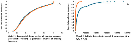
Figure 3.
Graphs of the two models discussed in the Methods Section. (A) Model 1 is based on an exponential decay that inversely relates to the frequency of road crossings by an animal. Since the core parameter, ‘frequency,’ remains unchanged across the two traffic conditions, and the same seed random number generator is used, the resulting curves almost overlap. (B) Model 2 utilizes a 7-parameter horizontal ballistic model. In this case, the Monte Carlo-simulated data (per equation) differs between the two traffic conditions, despite using the same seed random number generator as in Model 1.
3.2. Model Comparison and Statistical Testing (Hypothesis 1)
The null hypothesis when comparing the two models is that the observed likelihoods L1 and L2 (Figure 3A,B) do not differ significantly, implying that there is no effect or issue arising from their structure.
As shown in Appendix B, the test statistic employed, −2log (L1/L2), is compared to the critical value from the χ2 distribution with six degrees of freedom. The simulated data distribution used is Δ[(k − kl) − (k* − kl*)] (see Table 2), which is 2000 data points long since the following is true:
The overall variance of Δ[(k − kl) − (k* − kl*)] = 0.066, the degrees of freedom = 6, and the corresponding critical value of the χ2 distribution = 12.59. For the ratio λ,
And the test statistic −2log(L2/L1) = 7.31. Since the resulting test statistic (7.31) falls below the critical χ2 threshold, the null hypothesis cannot be rejected. This indicates that the models are not statistically distinguishable in terms of likelihood under the given simulated conditions.
A visual examination of Figure 3A,B further corroborates the statistical outcome. Both models produced smooth, unimodal distributions of likelihood values across simulated traffic densities. The probability surfaces exhibited overlapping confidence regions, particularly between traffic density values of 0.4 and 0.6, with no indication of skewness, multimodality, or abrupt inflections. Residual analysis revealed no localized clustering or anomalies.
Moreover, dispersion patterns were relatively symmetric and homoscedastic across the simulation space. The likelihood ratio (λ) remained stable across a wide range of input parameters, suggesting that the differences in structural formulation between the two models do not translate into meaningful divergence in predicted WVC likelihood.
In sum, the statistical and graphical analyses jointly demonstrate that the models, despite differing in their mechanistic underpinnings, yield comparable outputs under equivalent traffic conditions. As such, this result supports the null hypothesis: that no significant structural effect emerges between the two model frameworks when applied to simulated data derived from identical environmental and traffic parameters.
3.3. Model Divergence Under Traffic Regimes (Hypothesis 2)
Figure 4 illustrates the distribution of differences in likelihood values generated by Model 2 (L2, Equation (9)) under two traffic conditions normal and restricted conditions—as represented by Δ(k − kl). The cumulative relative frequency curve reveals a strongly left-skewed distribution, indicating that the majority of likelihood differences are slightly positive. In other words, most simulated values suggest that WVC likelihood is lower during lockdown traffic conditions.
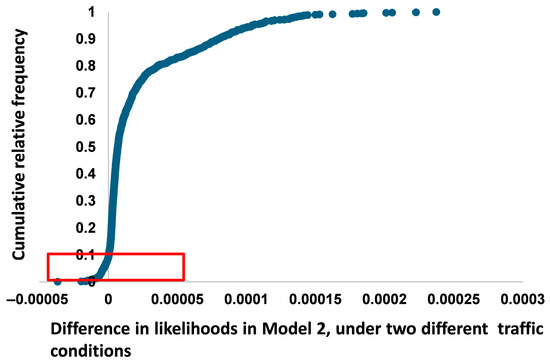
Figure 4.
Likelihood difference for Model 2 (L2, Equation (9)) under normal and restricted traffic conditions. The values highlighted in red in the sidebar represent the simulated data, showing that the likelihood of a wildlife–vehicle collision (WVC) event is greater under restricted mobility conditions than normal traffic conditions.
However, in 93 out of 1000 simulated cases (9.3%), the difference in likelihood is negative, meaning the model predicts a higher risk of wildlife–vehicle collisions under restricted traffic conditions. These cases appear as outliers on the distribution plot and are highlighted in red in the sidebar of Figure 4. The negative Δ(k − kl) values range from approximately −0.000027 to −0.0000014, with the majority of these concentrated around the lower tail of the distribution.
The steep increase in the cumulative frequency curve just after Δ = 0 confirms the rarity but statistical presence of these negative values. The interquartile range of Δ(k − kl) spans from 0.0000057 to 0.0000141, with a median value of 0.0000092, indicating a slight overall tendency toward positive likelihood differences. The minimum and maximum Δ values in the full sample range from −0.000027 to +0.000051. This outcome provides statistical support for the alternative hypothesis—that reductions in traffic do not universally reduce collision risk, and that certain ranges of traffic density may be associated with elevated WVC likelihood.
3.4. Sensitivity Analysis and Key Predictors (Hypothesis 3)
Figure 5 illustrates the results from the sensitivity analysis conducted on Model 2, which enhances the overall analysis presented in this study. The findings are significant in understanding the primary factors that contribute to variations in WVC events under different traffic conditions. This analysis clarifies the nuanced relationship between the commonly held belief that “fewer vehicles equals fewer WVCs” and the essential consideration that a driver’s behavior also plays a crucial role in such incidents. For example, under restricted traffic conditions, 17.6% of WVC events are attributed to higher vehicle speeds in low-congestion scenarios, while only 3.5% are linked to driver alertness. These findings support the interpretation by Stiles et al. [36], which states that “lower volumes lead to higher speeds”. This relationship can significantly alter both the type and severity of road crashes, particularly in the context of lockdown policies enacted during the COVID-19 pandemic.
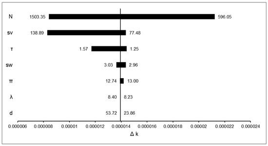
Figure 5.
Sensitivity analysis of the likelihood difference for Model 2 (L2, Equation (9)) under normal and restricted traffic conditions. Although the number of circulating vehicles is in first position and fewer vehicles influences the overall result of WVCs, the vehicle speed (sv) and the driver’s reaction time (τ) have a drastic influence on the overall model outputs.
In terms of contribution to Δk, the number of circulating vehicles (N) produced the largest effect, shifting likelihood values by more than 1.6 × 10⁻⁵. Vehicle speed (sv) followed, altering Δk by roughly 1.2 × 10⁻⁵, while driver reaction time (τ) contributed changes of about 8 × 10⁻⁶. In contrast, animal speed (sw), encounter probability (π), vehicle spacing (λ), and crossing distance (d) had comparatively smaller effects, with Δk shifts typically below 4 × 10⁻⁶.
Overall, all three hypotheses tested are supported by the simulated data. The results collectively validate the feasibility of an alternative generalization for WVC dynamics, offering a nuanced understanding that goes beyond the simplistic “fewer vehicles = fewer collisions” paradigm.
4. Discussion
Wildlife–vehicle collisions (WVCs) are typically documented only after they occur, based on field evidence or mortality records. By accumulating data on WVCs under specific environmental conditions, road and traffic factors, seasonal or diurnal variations, and animal roaming behavior [42,43,44,45,46], researchers can identify hotspots where the risk of WVCs is significantly elevated [47,48,49,50,51]. Such empirical knowledge, along with technical and safety specifications, constitutes the bulk of conservation measures that mitigate excessive mortality for certain flag species at a local scale, or in motorways crossing landscapes and ecosystems of conservation importance [29,39,52,53,54,55,56,57,58].
Animal road mortality is a significant conservation issue that also raises concerns about road safety. Numerous studies have documented WVC monitoring schemes in various countries and settings [59]. These schemes provide a foundation for assessing the severity of the WVC problem and highlight the efforts of conservationists to incorporate technical and safety specifications into road infrastructure planning to mitigate its impact. Importantly, such schemes also contribute to the detection and documentation of rare or poorly studied species, offering crucial records of distribution or presence in otherwise under-surveyed regions [60,61]. In Tier 4 countries (formerly known as developed countries), particularly in Europe, this issue is closely linked to the effects of modernization and the strategy for trans-European connection infrastructures, such as motorways, train networks, pipelines, and powerlines. The examples presented in the previous sections were intended to highlight a primary weakness of the WVC reports: the confusion between the probability and likelihood of a WVC event. Published results refer to observed WVC outcomes, denoted by O, without practically considering the set of parameters of the ‘vehicle(s)–motorway–animal(s)’ system and the real-life stochastic WVC process, denoted by θ. Then, the Anthropause argument reduces the estimate θ—that would be a plausible choice given the observed outcomes O—to the circular ‘fewer vehicles—fewer casualties’, which has already been proven weak in real-life lockdown conditions [36]. Addressing the WVC conservation challenge involves minimizing the probability P(O|θ) or maximizing L(θ|O) and not accurately recording O.
The second challenge related to thought arises from the fact that the COVID-19 pandemic, its duration, and the public health restrictions on human mobility did not unfold in a neutral or process-wise stable environmental context. Processes of modernization, such as urbanization and industrialization, along with rural depopulation, land abandonment, and the concentration of agricultural activities on fertile land, create circumstances that facilitate forest recovery [62]. In many European countries, the migration of rural populations to urban centers, the abandonment of remote villages, and the decline of small-scale local agriculture contribute to this recovery, as predicted by the Forest Transition Theory [62,63]. Additionally, the literature indicates a notable trend of wild animal recovery that coincides with the recovery of forests [64], as many species—including various ungulates, carnivores, and forest-dwelling birds—are known to recolonize regenerating habitats once ecological conditions become favorable.
A crucial aspect often overlooked in the literature is the lack of comparability in baseline conditions over time. When examining data that spans several decades (e.g., 10 to 30 years) to assess the severity of wildlife–vehicle collisions (WVCs), it is essential to recalibrate at least three core variables: (1) the size of the at-risk population has significantly increased; (2) the available habitat and foraging areas have expanded; (3) the road network has developed significantly; and (4) the likelihood of WVCs is affected by these first three factors. These long-term ecological shifts have direct implications for model assumptions and parameterization. Increases in wildlife population density, habitat expansion near roads, and new road infrastructure change both the spatial probability of animal–road encounters and the frequency of crossing events. If these factors are not integrated or updated in model inputs, predictions may become decoupled from real-world dynamics. Therefore, temporal comparability and ecological realism must be carefully considered when using WVC data across multi-decadal periods for model calibration and interpretation.
In Greece, for example, modernization has significantly transformed the rural landscape. In the 1960s, the rural population accounted for 44% of the total, but by 2020, this figure had dropped to 20%, a decline that is not attributed to the COVID-19 pandemic and continues to decrease. In terms of forested areas, the percentage was 30% in 2010; however, recent publications of forest cadastral surveys have raised this figure to 62%. This change reflects the abandonment of rural land and the natural recovery of forested regions. As a result, the recovery of wildlife populations, such as brown bears, wild boars, wolves, and jackals, has been remarkable. To calculate the percentage of road mortality for these species, we need to establish a baseline population size. For instance, the estimated population of brown bears in Greece was between 100 and 120 individuals 20 to 25 years ago. The current population is estimated to be approximately 500 individuals [41]. The ratio of bear–vehicle collisions to the total population indicates the percentage of road mortality of this emblematic species. However, we need to clarify which population estimate should be used as the denominator in this calculation. For instance, it is quite infeasible to calculate the yearly number of individuals added to the total population.
This demographic shift—marked by rural depopulation and wildlife resurgence—has altered the spatial risk of road collisions. As wild fauna recolonize rural and peri-urban landscapes, the probability of WVCs increases. In parallel, vehicle–human collisions (HVCs), more frequent in urban areas, continue to pose serious safety concerns for pedestrians and cyclists. Though these two types of collisions differ in their ecological and geographic contexts, both are shaped by overlapping behavioral and infrastructural risk factors.
Understanding the causes of these events is therefore essential for informed road safety and conservation strategies. The main causes of WVCs include the following: (1) driving above the speed limit or too fast for road conditions, which reduces drivers’ reaction times and increases the likelihood of collisions; (2) impairment from alcohol and drugs, which affects judgment, coordination, and reaction times; and (3) drowsy driving, which can be just as dangerous as driving under the influence. In urban areas, pedestrians and cyclists face higher risks due to additional factors. A significant issue is the lack of proper infrastructure, such as sidewalks and bike lanes, which exacerbates this risk. Additionally, behaviors like running red lights and illegal overtaking are frequent causes of fatal collisions.
Beyond case-specific explanations, these observations call for a rethinking of how WVCs are conceptualized and modeled. The reliance on retrospective interpretation reveals a significant limitation common in much of the Anthropause literature: an overwhelming dependence on observational data without predictive frameworks. Within this context, two alternative approaches emerge for interpreting the varied outcomes of wildlife–vehicle collisions (WVCs) during lockdowns. The first approach follows the classical legal maxim, “Exceptio probat regulam in casibus non exceptis,” meaning that the exception proves the rule in cases not excluded. This principle, established in English law in the early 17th century, suggests that the existence of an exception implies a general rule applicable to all other cases. From this perspective, deviations from the expected pattern of “fewer vehicles leads to fewer WVCs” are seen as outliers. The second, more critical perspective questions whether these exceptions indicate a need for a revised understanding—one that can accommodate multiple causal mechanisms, nonlinear interactions, and species-specific behavioral dynamics. This rethinking requires a shift from merely correlational inferences to mechanistic modeling rooted in the physics and biology of wildlife–vehicle interactions [25]. From a conservation modeling perspective, this raises a foundational question: can WVCs be conceptualized as a deterministic outcome of a kinematic (ballistic) interception problem, governed not solely by traffic volume, but by the spatiotemporal dynamics of both vehicles and animals? Under such a framework, key parameters would include vehicle speed, inter-vehicle spacing, traffic density, and road width, as well as animal behavior, such as daily movement rates, crossing attempts, and habitat use near roads. Ideally, such a system could be formalized into a dimensionless metric that represents the ratio of two distances (the distance an animal needs to cross versus the distance a vehicle travels) or two speeds (the speed of the car compared to the speed of the animal) along intersecting trajectories.
Yet, despite these known causes, predictive modeling of WVCs remains limited. This gap is partially due to the post hoc nature of data collection, where the spatial and temporal patterns of WVCs are retrospectively analyzed without fully integrating mechanistic or behavioral models. The simulation-based approach presented in this study—particularly Model 2—was developed to address precisely this gap by offering a physics-based interpretation of WVC dynamics grounded in real-world constraints.
While our formulations mark a step forward, we acknowledge that the current models remain theoretical and require empirical validation to assess their predictive performance under actual field conditions. Future work will apply these formulations to multi-year datasets of wildlife–vehicle collisions collected across Mediterranean landscapes, especially in regions with species-specific mortality records and detailed traffic parameters [24,45]. Empirical testing will be essential for evaluating the generalizability of both the ballistic and behavior-based models and for refining parameter estimates across varying ecological and infrastructural scenarios.
Furthermore, the present models intentionally focus on core mechanical and behavioral determinants of collision risk—primarily vehicle dynamics and simplified road-crossing behavior. However, several ecological and anthropogenic variables could significantly modulate WVC likelihood. These include species-specific traits such as diel activity, movement speed, or road avoidance, as well as seasonal behavior shifts linked to migration, breeding, or dispersal. On the human side, factors such as driver fatigue, distraction, and variability in hazard perception—beyond the parameterization of reaction time—can also influence collision probability. Although these components were not incorporated in the present framework, future model iterations could integrate such variables as adjustable parameters or probability distributions, enhancing ecological realism and scenario-specific applicability. We argue that segmented policies—technical improvements for conservation on one hand and urban safety interventions on the other—are unlikely to yield comprehensive results. Instead, WVCs must be integrated into broader transportation safety frameworks. The European Commission’s road safety strategy for 2021–2030 and the ‘Vision Zero’ initiative, which aims for zero road fatalities by 2050, provide an opportunity for this integration [65].
To this end, future policy must be informed by models capable of predicting WVC risk across varying traffic scenarios and ecological contexts. The use of probabilistic and mechanistic models, as demonstrated in our approach, is a necessary step toward this goal. Additionally, integrating real-time traffic data and animal movement data into such models would enhance their precision and practical utility.
Within this evolving technological landscape, the models developed here serve not as fixed constructs, but as adaptable frameworks. Grounded in biomechanical and behavioral principles, they provide a scalable foundation for incorporating additional ecological and anthropogenic variables as new data become available. This structural flexibility ensures that predictive accuracy can improve over time, facilitating a gradual shift from observational generalizations to dynamic, evidence-based forecasting. As such models mature, they could be integrated into decision support systems at national road agencies or environmental ministries. For instance, the probabilistic outputs can inform risk zoning along motorways where targeted mitigation (e.g., fencing, overpasses) is more likely to yield conservation gains. Furthermore, emerging machine learning pipelines now enable the real-time ingestion of GPS-tagged animal data and road traffic feeds, offering future opportunities for automated WVC prediction frameworks.
5. Conclusions
This study challenges the simplistic assumption that reduced traffic volume inherently leads to fewer wildlife–vehicle collisions. By modeling collision likelihoods as stochastic outcomes influenced by a suite of behavioral, mechanical, and environmental parameters, we offer a more nuanced framework for understanding road mortality during events such as the COVID-19 lockdowns. The two models developed here—one based on exponential decay of crossing attempts and another on a mechanistic ballistic interpretation—highlight the nonlinearity and complexity of WVC dynamics.
Our results demonstrate that, in a notable subset of scenarios, reduced vehicle numbers can paradoxically increase WVC risk, primarily due to elevated vehicle speeds and reduced driver vigilance in low-congestion environments. This finding underscores the need to shift from post hoc reporting of WVC counts to predictive, likelihood-based modeling that can inform dynamic traffic policy.
The implications are both scientific and policy-oriented: model-based WVC forecasting tools should be embedded within transport safety strategies, especially those aspiring to reach the European Commission’s ‘Vision Zero’ target. Based on our findings, we recommend: (1) incorporating traffic density thresholds into road safety planning, acknowledging that WVC risk may increase at intermediate traffic volumes; (2) prioritizing dynamic speed regulation in areas with known wildlife activity, especially during periods of reduced traffic when higher vehicular speeds are more likely; (3) implementing species-specific mitigation (e.g., fencing, crossing structures) informed by local traffic and animal movement patterns; and (4) integrating driver behavior parameters, such as reaction time and vehicle spacing, into future collision risk assessments.
Future work should focus on validating these recommendations across different biogeographical contexts, enhancing them with real-time data streams, and coupling them with habitat and movement ecology to ensure ecologically meaningful mitigation.
Author Contributions
Conceptualization, A.Y.T.; methodology, A.Y.T.; software, A.Y.T.; validation, A.Y.T. and Y.G.Z.; formal analysis A.Y.T.; investigation, Y.G.Z.; resources, A.Y.T. and Y.G.Z.; data curation, A.Y.T. and Y.G.Z.; writing—original draft preparation, A.Y.T.; writing—review and editing, A.Y.T. and Y.G.Z.; visualization, A.Y.T. All authors have read and agreed to the published version of the manuscript.
Funding
This research received no external funding.
Institutional Review Board Statement
Not applicable.
Data Availability Statement
Data is contained within the article.
Acknowledgments
We dedicate this work to the loving memory of our colleague Niki Georgi, who passed away during the final stages of this study. A devoted member of our Department and a steadfast presence in the Biodiversity Conservation Laboratory, Niki supported us—and generations of students and colleagues—with unwavering care, professionalism, and kindness. Whether helping in the lab, preparing field materials, or simply offering quiet encouragement, her presence shaped our daily academic life in ways both big and small. May her memory continue to inspire through the students she guided and the knowledge she helped nurture.
Conflicts of Interest
The authors declare no conflicts of interest.
Appendix A
We are given the following equation: . We take the natural logarithm of both sides:
We divide both sides by n:
We exponentiate both sides:
We solve for k:
The reason we say “approximately” is that, in practice, we might use this formula in contexts where k is estimated or where the expression is part of a larger approximation.
Appendix B
The chi-square test (χ2) for homogeneity compares distributions across different populations. The likelihood ratio test (LRT) statistic compares two models: L1, which expresses the likelihood of the data under the null hypothesis, and L2, the likelihood under the alternative hypothesis. The formula is as follows:
This statistic approximately follows a χ2 distribution under the null hypothesis, with degrees of freedom equal to the difference in the number of parameters between the two models.
References
- Grilo, C.; Koroleva, E.; Andrášik, R.; Bíl, M.; González-Suárez, M. Roadkill risk and population vulnerability in European birds and mammals. Front. Ecol. Environ. 2020, 18, 323–328. [Google Scholar] [CrossRef]
- Langbein, J.; Putman, R.; Pokorny, B. Traffic collisions involving deer and other ungulates in Europe and available measures for mitigation. In Ungulate Management in Europe; Cambridge University Press: Cambridge, UK, 2011; pp. 215–259. ISBN 9780511974137. [Google Scholar]
- Linnell, J.D.C.; Cretois, B.; Nilsen, E.B.; Rolandsen, C.M.; Solberg, E.J.; Veiberg, V.; Kaczensky, P.; Van Moorter, B.; Panzacchi, M.; Rauset, G.R.; et al. The challenges and opportunities of coexisting with wild ungulates in the human-dominated landscapes of Europe’s Anthropocene. Biol. Conserv. 2020, 244, 108500. [Google Scholar] [CrossRef]
- Kadmon, B. Uncovering the Truth About Moloch: Separating Fact from Fiction; Independently Published: Chicago, IL, USA, 2023; ISBN 979-8376404836. [Google Scholar]
- Ibisch, P.L.; Hoffmann, M.T.; Kreft, S.; Pe’Er, G.; Kati, V.; Biber-Freudenberger, L.; DellaSala, D.A.; Vale, M.M.; Hobson, P.R.; Selva, N. A global map of roadless areas and their conservation status. Science 2016, 354, 1423–1427. [Google Scholar] [CrossRef]
- Grilo, C.; Borda-de-Água, L.; Beja, P.; Goolsby, E.; Soanes, K.; le Roux, A.; Koroleva, E.; Ferreira, F.Z.; Gagné, S.A.; Wang, Y.; et al. Conservation threats from roadkill in the global road network. Glob. Ecol. Biogeogr. 2021, 30, 2200–2210. [Google Scholar] [CrossRef]
- Rutz, C.; Loretto, M.-C.; Bates, A.E.; Davidson, S.C.; Duarte, C.M.; Jetz, W.; Johnson, M.; Kato, A.; Kays, R.; Mueller, T.; et al. COVID-19 lockdown allows researchers to quantify the effects of human activity on wildlife. Nat. Ecol. Evol. 2020, 4, 1156–1159. [Google Scholar] [CrossRef] [PubMed]
- Jones, N.; McGinlay, J.; Jones, A.; Malesios, C.; Holtvoeth, J.; Dimitrakopoulos, P.G.; Gkoumas, V.; Kontoleon, A. COVID-19 and protected areas: Impacts, conflicts, and possible management solutions. Conserv. Lett. 2021, 14, e12800. [Google Scholar] [CrossRef]
- Corlett, R.T.; Primack, R.B.; Devictor, V.; Maas, B.; Goswami, V.R.; Bates, A.E.; Koh, L.P.; Regan, T.J.; Loyola, R.; Pakeman, R.J.; et al. Impacts of the coronavirus pandemic on biodiversity conservation. Biol. Conserv. 2020, 246, 108571. [Google Scholar] [CrossRef]
- Schwartz, M.W.; Glikman, J.A.; Cook, C.N. The COVID-19 pandemic: A learnable moment for conservation. Conserv. Sci. Pract. 2020, 2, e255. [Google Scholar] [CrossRef]
- Bates, A.E.; Primack, R.B.; Moraga, P.; Duarte, C.M. COVID-19 pandemic and associated lockdown as a “Global Human Confinement Experiment” to investigate biodiversity conservation. Biol. Conserv. 2020, 248, 108665. [Google Scholar] [CrossRef]
- Perkins, S.E.; Shilling, F.; Collinson, W. Anthropause Opportunities: Experimental Perturbation of Road Traffic and the Potential Effects on Wildlife. Front. Ecol. Evol. 2022, 10, 833129. [Google Scholar] [CrossRef]
- Primack, R.B.; Bates, A.E.; Duarte, C.M. The conservation and ecological impacts of the COVID-19 pandemic. Biol. Conserv. 2021, 260, 109204. [Google Scholar] [CrossRef]
- Bates, A.E.; Primack, R.B.; Biggar, B.S.; Bird, T.J.; Clinton, M.E.; Command, R.J.; Richards, C.; Shellard, M.; Geraldi, N.R.; Vergara, V.; et al. Global COVID-19 lockdown highlights humans as both threats and custodians of the environment. Biol. Conserv. 2021, 263, 109175. [Google Scholar] [CrossRef]
- Balčiauskas, L.; Kučas, A.; Balčiauskienė, L. Mammal Roadkills in Lithuanian Urban Areas: A 15-Year Study. Animals 2023, 13, 3272. [Google Scholar] [CrossRef]
- Łopucki, R.; Kitowski, I.; Perlińska-Teresiak, M.; Klich, D. How Is Wildlife Affected by the COVID-19 Pandemic? Lockdown Effect on the Road Mortality of Hedgehogs. Animals 2021, 11, 868. [Google Scholar] [CrossRef]
- Pokorny, B.; Cerri, J.; Bužan, E. Wildlife roadkill and COVID-19: A biologically significant, but heterogeneous, reduction. J. Appl. Ecol. 2022, 59, 1291–1301. [Google Scholar] [CrossRef]
- Bíl, M.; Heigl, F.; Janoška, Z.; Vercayie, D.; Perkins, S.E. Benefits and challenges of collaborating with volunteers: Examples from National Wildlife Roadkill Reporting Systems in Europe. J. Nat. Conserv. 2020, 54, 125798. [Google Scholar] [CrossRef]
- Kishimoto, K.; Kobori, H. COVID-19 pandemic drives changes in participation in citizen science project “City Nature Challenge” in Tokyo. Biol. Conserv. 2021, 255, 109001. [Google Scholar] [CrossRef]
- Vardi, R.; Berger-Tal, O.; Roll, U. iNaturalist insights illuminate COVID-19 effects on large mammals in urban centers. Biol. Conserv. 2021, 254, 108953. [Google Scholar] [CrossRef]
- Basile, M.; Russo, L.F.; Russo, V.G.; Senese, A.; Bernardo, N. Birds seen and not seen during the COVID-19 pandemic: The impact of lockdown measures on citizen science bird observations. Biol. Conserv. 2021, 256, 109079. [Google Scholar] [CrossRef]
- Sánchez-Clavijo, L.M.; Martínez-Callejas, S.J.; Acevedo-Charry, O.; Diaz-Pulido, A.; Gómez-Valencia, B.; Ocampo-Peñuela, N.; Ocampo, D.; Olaya-Rodríguez, M.H.; Rey-Velasco, J.C.; Soto-Vargas, C.; et al. Differential reporting of biodiversity in two citizen science platforms during COVID-19 lockdown in Colombia. Biol. Conserv. 2021, 256, 109077. [Google Scholar] [CrossRef]
- Waetjen, D.; Shilling, F. Impact of COVID-19 on Traffic, Crashes, and Wildlife-Vehicle Collisions. In Proceedings of the International Conference on Ecology and Transportation (ICOET), Denver, CO, USA, 11–15 May 2025. [Google Scholar]
- Kouris, A.D.; Christopoulos, A.; Vlachopoulos, K.; Christopoulou, A.; Dimitrakopoulos, P.G.; Zevgolis, Y.G. Spatiotemporal Patterns of Reptile and Amphibian Road Fatalities in a Natura 2000 Area: A 12-Year Monitoring of the Lake Karla Mediterranean Wetland. Animals 2024, 14, 708. [Google Scholar] [CrossRef]
- Troumbis, A.Y.; Zevgolis, Y.G. Beyond Circumstantial Evidence on Wildlife–Vehicle Collisions During COVID-19 Lockdown: A Deterministic vs. Probabilistic Multi-Year Analysis from a Mediterranean Island. Ecologies 2025, 6, 42. [Google Scholar] [CrossRef]
- Bíl, M.; Andrášik, R.; Cícha, V.; Arnon, A.; Kruuse, M.; Langbein, J.; Náhlik, A.; Niemi, M.; Pokorny, B.; Colino-Rabanal, V.J.; et al. COVID-19 related travel restrictions prevented numerous wildlife deaths on roads: A comparative analysis of results from 11 countries. Biol. Conserv. 2021, 256, 109076. [Google Scholar] [CrossRef]
- LeClair, G.; Chatfield, M.W.H.; Wood, Z.; Parmelee, J.; Frederick, C.A. Influence of the COVID-19 pandemic on amphibian road mortality. Conserv. Sci. Pract. 2021, 3, e535. [Google Scholar] [CrossRef]
- Basak, S.M.; O’Mahony, D.T.; Lesiak, M.; Basak, A.K.; Ziółkowska, E.; Kaim, D.; Hossain, M.S.; Wierzbowska, I.A. Animal-vehicle collisions during the COVID-19 lockdown in early 2020 in the Krakow metropolitan region, Poland. Sci. Rep. 2022, 12, 7572. [Google Scholar] [CrossRef]
- Asari, Y. Decreased traffic volume during COVID-19 did not reduce roadkill on fenced highway network in Japan. Landsc. Ecol. Eng. 2022, 18, 121–124. [Google Scholar] [CrossRef]
- Abraham, J.O.; Mumma, M.A. Elevated wildlife-vehicle collision rates during the COVID-19 pandemic. Sci. Rep. 2021, 11, 20391. [Google Scholar] [CrossRef]
- Yasin, Y.J.; Grivna, M.; Abu-Zidan, F.M. Global impact of COVID-19 pandemic on road traffic collisions. World J. Emerg. Surg. 2021, 16, 51. [Google Scholar] [CrossRef]
- Department for Transport Reported Road Casualties Great Britain, Annual Report. Available online: https://www.gov.uk/government/statistics/reported-road-casualties-great-britain-annual-report-2020/reported-road-casualties-great-britain-annual-report-2020 (accessed on 15 April 2025).
- Office of Behavioral Safety Research Update to Special Reports on Traffic Safety During the COVID-19 Public Health Emergency: Third Quarter Data (Report No. DOT HS 813 069). Available online: https://www.nhtsa.gov/sites/nhtsa.gov/files/documents/traffic_safety_during_covid19_01062021_0.pdf (accessed on 15 April 2025).
- Chowdhury, D. Statistical physics of vehicular traffic and some related systems. Phys. Rep. 2000, 329, 199–329. [Google Scholar] [CrossRef]
- Nagatani, T. Traffic dispersion and its mapping to one-sided ballistic deposition. Phys. A Stat. Mech. Appl. 2007, 376, 641–648. [Google Scholar] [CrossRef]
- Stiles, J.; Kar, A.; Lee, J.; Miller, H.J. Lower Volumes, Higher Speeds: Changes to Crash Type, Timing, and Severity on Urban Roads from COVID-19 Stay-at-Home Policies. Transp. Res. Rec. J. Transp. Res. Board 2023, 2677, 15–27. [Google Scholar] [CrossRef]
- Pagany, R. Wildlife-vehicle collisions—Influencing factors, data collection and research methods. Biol. Conserv. 2020, 251, 108758. [Google Scholar] [CrossRef]
- Shilling, F.; Collinson, W.; Bil, M.; Vercayie, D.; Heigl, F.; Perkins, S.E.; MacDougall, S. Designing wildlife-vehicle conflict observation systems to inform ecology and transportation studies. Biol. Conserv. 2020, 251, 108797. [Google Scholar] [CrossRef]
- Spanowicz, A.G.; Teixeira, F.Z.; Jaeger, J.A.G. An adaptive plan for prioritizing road sections for fencing to reduce animal mortality. Conserv. Biol. 2020, 34, 1210–1220. [Google Scholar] [CrossRef]
- Zevgolis, Y.G.; Kouris, A.D.; Christopoulos, A.; Leros, M.; Loupou, M.; Rammou, D.-L.; Youlatos, D.; Troumbis, A.Y. Where to Protect? Spatial Ecology and Conservation Prioritization of the Persian Squirrel at the Westernmost Edge of Its Distribution. Land 2025, 14, 876. [Google Scholar] [CrossRef]
- Psaralexi, M.; Lazarina, M.; Mertzanis, Y.; Michaelidou, D.-E.; Sgardelis, S. Exploring 15 years of brown bear (Ursus arctos)-vehicle collisions in northwestern Greece. Nat. Conserv. 2022, 47, 105–119. [Google Scholar] [CrossRef]
- Rocha, L.M.D.; Rosa, C.; Secco, H.; Lopes, E.V. Hotspots and hotmoments of wildlife roadkills along a main highway in a high biodiversity area in Brazilian Amazonia. Acta Amaz. 2023, 53, 42–52. [Google Scholar] [CrossRef]
- Cook, T.C.; Blumstein, D.T. The omnivore’s dilemma: Diet explains variation in vulnerability to vehicle collision mortality. Biol. Conserv. 2013, 167, 310–315. [Google Scholar] [CrossRef]
- Sillero, N.; Poboljšaj, K.; Lešnik, A.; Šalamun, A. Influence of Landscape Factors on Amphibian Roadkills at the National Level. Diversity 2019, 11, 13. [Google Scholar] [CrossRef]
- Zevgolis, Y.G.; Kouris, A.; Christopoulos, A. Spatiotemporal Patterns and Road Mortality Hotspots of Herpetofauna on a Mediterranean Island. Diversity 2023, 15, 478. [Google Scholar] [CrossRef]
- Nguyen, H.K.D.; Fielding, M.W.; Buettel, J.C.; Brook, B.W. Predicting spatial and seasonal patterns of wildlife–vehicle collisions in high-risk areas. Wildl. Res. 2022, 49, 428–437. [Google Scholar] [CrossRef]
- Shilling, F.M.; Waetjen, D.P. Wildlife-vehicle collision hotspots at US highway extents: Scale and data source effects. Nat. Conserv. 2015, 11, 41–60. [Google Scholar] [CrossRef]
- Snow, N.P.; Williams, D.M.; Porter, W.F. A landscape-based approach for delineating hotspots of wildlife-vehicle collisions. Landsc. Ecol. 2014, 29, 817–829. [Google Scholar] [CrossRef]
- Bencin, H.L.; Prange, S.; Rose, C.; Popescu, V.D. Roadkill and space use data predict vehicle-strike hotspots and mortality rates in a recovering bobcat (Lynx rufus) population. Sci. Rep. 2019, 9, 15391. [Google Scholar] [CrossRef]
- Canal, D.; Camacho, C.; Martín, B.; de Lucas, M.; Ferrer, M. Fine-scale determinants of vertebrate roadkills across a biodiversity hotspot in Southern Spain. Biodivers. Conserv. 2019, 28, 3239–3256. [Google Scholar] [CrossRef]
- Valerio, F.; Basile, M.; Balestrieri, R. The identification of wildlife-vehicle collision hotspots: Citizen science reveals spatial and temporal patterns. Ecol. Process. 2021, 10, 6. [Google Scholar] [CrossRef]
- Ascensão, F.; Yogui, D.R.; Alves, M.H.; Alves, A.C.; Abra, F.; Desbiez, A.L.J. Preventing wildlife roadkill can offset mitigation investments in short-medium term. Biol. Conserv. 2021, 253, 108902. [Google Scholar] [CrossRef]
- Zimmermann Teixeira, F.; Kindel, A.; Hartz, S.M.; Mitchell, S.; Fahrig, L. When road-kill hotspots do not indicate the best sites for road-kill mitigation. J. Appl. Ecol. 2017, 54, 1544–1551. [Google Scholar] [CrossRef]
- Plante, J.; Jaeger, J.A.G.; Desrochers, A. How do landscape context and fences influence roadkill locations of small and medium-sized mammals? J. Environ. Manag. 2019, 235, 511–520. [Google Scholar] [CrossRef]
- Assis, J.C.; Giacomini, H.C.; Ribeiro, M.C. Road Permeability Index: Evaluating the heterogeneous permeability of roads for wildlife crossing. Ecol. Indic. 2019, 99, 365–374. [Google Scholar] [CrossRef]
- Van Niekerk, A.; Eloff, P.J. Game, fences and motor vehicle accidents: Spatial patterns in the Eastern Cape. S. Afr. J. Wildl. Res. 2005, 35, 125–130. [Google Scholar]
- Patrick, D.A.; Schalk, C.M.; Gibbs, J.P.; Woltz, H.W. Effective Culvert Placement and Design to Facilitate Passage of Amphibians across Roads. J. Herpetol. 2010, 44, 618–626. [Google Scholar] [CrossRef]
- Pinto, C.M.; Vargas Soto, J.S.; Flatt, E.; Barboza, K.; Whitworth, A. Identifying wildlife road crossing mitigation sites using a multi-data approach—A case study from southwestern Costa Rica. J. Environ. Manag. 2024, 361, 121263. [Google Scholar] [CrossRef]
- Guinard, E.; Billon, L.; Bretaud, J.-F.; Chevallier, L.; Sordello, R.; Witté, I. Comparing the effectiveness of two roadkill survey methods on roads. Transp. Res. Part D Transp. Environ. 2023, 121, 103829. [Google Scholar] [CrossRef]
- Hwang, J.-W.; Jo, Y.-S. Wildlife–Vehicle Collisions and Mitigation: Current Status and Factor Analysis in South Korea. Animals 2024, 14, 3012. [Google Scholar] [CrossRef]
- Zevgolis, Y.G.; Kouris, A.D.; Zannetos, S.P.; Selimas, I.; Kontos, T.D.; Christopoulos, A.; Dimitrakopoulos, P.G.; Akriotis, T. Invasion Patterns of the Coypu, Myocastor coypus, in Western Central Greece: New Records Reveal Expanding Range, Emerging Hotspots, and Habitat Preferences. Land 2025, 14, 365. [Google Scholar] [CrossRef]
- Mather, A.S. The Forest Transition. Area 1992, 24, 367–379. [Google Scholar]
- Mather, A.S.; Needle, C.L. The forest transition: A theoretical basis. Area 1998, 30, 117–124. [Google Scholar] [CrossRef]
- Arts, K.; Fischer, A.; van der Wal, R. Boundaries of the wolf and the wild: A conceptual examination of the relationship between rewilding and animal reintroduction. Restor. Ecol. 2016, 24, 27–34. [Google Scholar] [CrossRef]
- European Commission Road Safety Statistics in the EU. Available online: https://ec.europa.eu/eurostat/statistics-explained/index.php?oldid=630784 (accessed on 8 February 2025).
Disclaimer/Publisher’s Note: The statements, opinions and data contained in all publications are solely those of the individual author(s) and contributor(s) and not of MDPI and/or the editor(s). MDPI and/or the editor(s) disclaim responsibility for any injury to people or property resulting from any ideas, methods, instructions or products referred to in the content. |
© 2025 by the authors. Licensee MDPI, Basel, Switzerland. This article is an open access article distributed under the terms and conditions of the Creative Commons Attribution (CC BY) license (https://creativecommons.org/licenses/by/4.0/).