
Can a Non-Destructive Method Predict the Leaf Area of Species in the Caatinga Biome?

 , , , , , , , , , , and
Abstract
1. Introduction
2. Materials and Methods
3. Results
4. Discussion
5. Conclusions
Author Contributions
Funding
Institutional Review Board Statement
Data Availability Statement
Acknowledgments
Conflicts of Interest
References
- Legris, M. Light and temperature regulation of leaf morphogenesis in Arabidopsis. New Phytol. 2023, 240, 2191–2196. [Google Scholar]
- Lusk, C.H.; Grierson, E.R.P.; Laughlin, D.C. Large leaves in warm, moist environments confer an advantage in seedling light interception efficiency. New Phytol. 2019, 223, 1319–1327. [Google Scholar]
- He, J.; Reddy, G.V.P.; Liu, M.; Shi, P. A general formula for calculating surface area of the similarly shaped leaves: Evidence from six Magnoliaceae species. Glob. Ecol. Conserv. 2020, 23, e01129. [Google Scholar]
- Macário, A.P.S.; Ferraz, R.L.d.S.; Costa, P.d.S.; Brito Neto, J.F.d.; Melo, A.S.d.; Dantas Neto, J. Allometric models for estimating Moringa oleifera leaflets area. Ciência Agrotecnologia 2020, 44, e005220. [Google Scholar] [CrossRef]
- Adji, B.I.; Akaffou, D.S.; Kouassi, K.H.; Houphouet, Y.P.; De Reffye, P.; Duminil, J.; Jaeger, M.; Sabatier, S. Allometric models for non-destructive estimation of dry biomass and leaf area in Khaya senegalensis (Desr.) A. Juss., 1830 (Meliaceae), Pterocarpus erinaceus Poir., 1804 (Fabaceae) and Parkia biglobosa, Jack, R. Br., 1830 (Fabaceae). Trees 2021, 35, 1905–1920. [Google Scholar] [CrossRef]
- Pohlmann, V.; Lago, I.; Lopes, S.J.; Martins, J.T.d.S.; da Rosa, C.A.; Caye, M.; Portalanza, D. Estimation of common bean (Phaseolus vulgaris) leaf area by a non-destructive method. Semin. Cienc. Agrar. 2021, 42, 2163–2180. [Google Scholar]
- Salazar, J.C.S.; Melgarejo, L.M.; Bautista, E.H.D.; Di Rienzo, J.A.; Casanoves, F. Non-destructive estimation of the leaf weight and leaf area in cacao (Theobroma cacao L.). Sci. Hortic. 2018, 229, 19–24. [Google Scholar] [CrossRef]
- Zhang, W. Digital image processing method for estimating leaf length and width tested using kiwifruit leaves (Actinidia chinensis Planch). PLoS ONE 2020, 15, e0235499. [Google Scholar]
- Adhikari, R.; Li, C.; Kalbaugh, K.; Nemali, K. A low-cost smartphone controlled sensor based on image analysis for estimating whole-plant tissue nitrogen (N) content in floriculture crops. Comput. Electron. Agric. 2020, 169, 105173. [Google Scholar] [CrossRef]
- Dias, M.G.; Silva, T.I.d.; Ribeiro, J.E.d.S.; Grossi, J.A.S.; Barbosa, J.G. Allometric models for estimating the leaf area of lisianthus (Eustoma grandiflorum) using a non-destructive method. Rev. Ceres 2022, 69, 7–12. [Google Scholar] [CrossRef]
- Ribeiro, J.E.S.; Coêlho, E.S.; Pessoa, A.M.S.; de Oliveira, A.K.S.; de Oliveira, A.M.F.; Barros Júnior, A.P.; Mendonça, V.; Nunes, G.S. Nondestructive method for estimating the leaf area of sapodilla from linear leaf dimensions. Rev. Bras. Eng. Agric. Ambient.-Agriambi 2023, 27, 209–215. [Google Scholar] [CrossRef]
- Silva, T.I.d.; Ribeiro, J.E.d.S.; Dias, M.G.; Cruz, R.R.P.; Macêdo, L.F.; Nóbrega, J.S.; Sales, G.N.B.; Santos, E.P.d.; Costa, F.B.d.; Grossi, J.A.S. Non-destructive method for estimating chrysanthemum leaf area. Rev. Bras. Eng. Agrícola Ambient. 2023, 27, 934–940. [Google Scholar] [CrossRef]
- De Sousa, S.K.A.; Nascimento, R.G.M.; Rodrigues, F.H.S.; Viana, R.G.; da Costa, L.C.; Pinheiro, H.A. Allometric models for non-destructive estimation of the leaflet area in acai (Euterpe oleracea Mart.). Trees 2024, 38, 169–178. [Google Scholar] [CrossRef]
- Hernández-Fernandéz, I.A.; Jarma-Orozco, A.; Pompelli, M.F. Allometric models for non-destructive leaf area measurement of stevia: An in depth and complete analysis. Hortic. Bras. 2021, 39, 205–215. [Google Scholar] [CrossRef]
- Da Silva Júnior, J.B.; da Silva, S.I.; de Medeiros, P.R.; de Oliveira, A.F.M. Potential oil resources from underutilized seeds of Cynophalla flexuosa (Capparaceae) from coastal and semiarid regions of Northeast Brazil. Biocatal. Agric. Biotechnol. 2023, 51, 102771. [Google Scholar] [CrossRef]
- E Silva, É.E.d.M.; Paixão, V.H.F.; Torquato, J.L.; Lunardi, D.G.; de Oliveira Lunardi, V. Fruiting phenology and consumption of zoochoric fruits by wild vertebrates in a seasonally dry tropical forest in the Brazilian Caatinga. Acta Oecologica 2020, 105, 103553. [Google Scholar] [CrossRef]
- Dos Santos Magalhães, C.; da Silva, F.C.L.; Randau, K.P. Comparative morphoanatomic, histochemical, and phytochemical characterization of leaves of two species of the genus Cynophalla (DC.) J. Presl. Biochem. Syst. Ecol. 2024, 114, 104830. [Google Scholar] [CrossRef]
- Almeida, N.C.O.S.; Silva, F.R.P.; Carneiro, A.L.B.; Lima, E.S.; Barcellos, J.F.M.; Furtado, S.C. Libidibia ferrea (jucá) anti-inflammatory action: A systematic review of in vivo and in vitro studies. PLoS ONE 2021, 16, e0259545. [Google Scholar] [CrossRef]
- Oliveira, F.G.; Santos, F.d.S.; Lewis, G.P.; de Oliveira, R.P.; de Queiroz, L.P. Reassessing the taxonomy of the Libidibia ferrea complex, the iconic Brazilian tree “pau-ferro” using morphometrics and ecological niche modeling. Braz. J. Bot. 2024, 47, 1203–1219. [Google Scholar] [CrossRef]
- De Paulo Pereira, L.; da Silva, R.O.; Bringel, P.H.d.S.F.; da Silva, K.E.S.; Assreuy, A.M.S.; Pereira, M.G. Polysaccharide fractions of Caesalpinia ferrea pods: Potential anti-inflammatory usage. J. Ethnopharmacol. 2012, 139, 642–648. [Google Scholar] [CrossRef]
- Freire, F.C.d.J.; Silva-Pinheiro, J.d.; Santos, J.S.; Silva, A.G.L.d.; Camargos, L.S.d.; Endres, L.; Justino, G.C. Proline and antioxidant enzymes protect Tabebuia aurea (Bignoniaceae) from transitory water deficiency. Rodriguésia 2022, 73, e02062020. [Google Scholar] [CrossRef]
- Almeida, R.d.S.; Moura, L.B.; Araújo, M.P.d.; Gomes, A.C.; Medeiros, J.G.F.; Dornelas, C.S.M.; Lacerda, A.V.d. Biometriy of Seeds of Tabebuia aurea (Silva Manso) Benth. & Hook. f. ex. S. Moore and Seedling Growth After Different Periods of Water Immersion. Braz. Arch. Biol. Technol. 2023, 66, e23220697. [Google Scholar]
- Guedes, R.S.; Alves, E.U.; Melo, P.A.F.R.d.; Moura, S.d.S.S.; Silva, R.d.S.d. Storage of Tabebuia caraiba (Mart.) Bureau seeds in different packaging and temperatures. Rev. Bras. De Sementes 2012, 34, 433–440. [Google Scholar] [CrossRef]
- Mahmoud, A.H.; Mahmoud, B.K.; Samy, M.N.; Fouad, M.A.; Kamel, M.S.; Matsunami, K. Cytotoxic and antileishmanial triterpenes of Tabebuia aurea (Silva Manso) leaves. Nat. Prod. Res. 2022, 36, 6181–6185. [Google Scholar] [CrossRef]
- Wijayanti, E.D.; Rahayu, L.O.; Raharjo, S.J.; Hayuningtyas, D.P.; Wulandari, D.; Maharani, A.D.; Maulidina, I.; Febrianti, R. Antimicrobial activity of yellow tabebuia flower extract (Tabebuia aurea) against drug-resistant microbes. Berk. Penelit. Hayati 2024, 30, 144–151. [Google Scholar] [CrossRef]
- Ribeiro, J.E.d.S.; Coêlho, E.d.S.; Figueiredo, F.R.A.; Melo, M.F. Non-destructive method for estimating leaf area of Erythroxylum pauferrense (Erythroxylaceae) from linear dimensions of leaf blades. Acta Botánica Mex. 2020, 127, e1717. [Google Scholar] [CrossRef]
- Boyacı, S.; Küçükönder, H. A research on non-destructive leaf area estimation modeling for some apple cultivars. Erwerbs-Obstbau 2022, 64, 1–7. [Google Scholar] [CrossRef]
- Cargnelutti Filho, A.; Pezzini, R.V.; Neu, I.M.M.; Dumke, G.E. Estimation of buckwheat leaf area by leaf dimensions. Semin. Cienc. Agrar. 2021, 42 (Suppl. 1), 1529–1548. [Google Scholar] [CrossRef]
- Goergen, P.C.H.; Lago, I.; Schwab, N.T.; Alves, A.F.; Freitas, C.P.d.O.; Selli, V.S. Allometric relationship and leaf area modeling estimation on chia by non-destructive method. Rev. Bras. Eng. Agrícola Ambient. 2021, 25, 305–311. [Google Scholar] [CrossRef]
- Rodriguez-Paez, L.A.; Jarma-Orozco, A.; Jaraba-Navas, J.d.D.; Pineda-Rodriguez, Y.Y.; Pompelli, M.F. Leaf Area Estimation of Yellow Oleander Thevetia peruviana (Pers.) K. Schum Using a Non-Destructive Allometric Model. Forests 2023, 15, 57. [Google Scholar] [CrossRef]
- Alvares, C.A.; Stape, J.L.; Sentelhas, P.C.; Gonçalves, J.L.d.M.; Sparovek, G. Köppen’s climate classification map for Brazil. Meteorol. Z. 2013, 22, 711–728. [Google Scholar] [CrossRef]
- Dos Santos, H.G.; Jacomine, P.K.T.; Dos Anjos, L.H.C.; De Oliveira, V.A.; Lumbreras, J.F.; Coelho, M.R.; De Almeida, J.A.; de Araujo Filho, J.C.; de Oliveira, J.B.d.; Cunha, T.J.F. Sistema Brasileiro de Classificação de Solos; Embrapa: Brasília, DF, Brazil, 2018. [Google Scholar]
- Marquaridt, D.W. Generalized inverses, ridge regression, biased linear estimation, and nonlinear estimation. Technometrics 1970, 12, 591–612. [Google Scholar]
- Gill, J.L. Outliers, residuals, and influence in multiple regression. Z. Fuer Tierzuechtung Und Zuechtungsbiologie 1986, 103, 161–175. [Google Scholar]
- R Core Team. R Development Core Team R: A Language and Environment for Statistical Computing 2023; R Core Team: Vienna, Austria, 2023. [Google Scholar]
- Junges, A.H.; Anzanello, R. Non-destructive simple model to estimate the leaf area through midvein in cultivars of Vitis vinifera. Rev. Bras. Frutic. 2021, 43, e-795. [Google Scholar]
- Da Silva Ribeiro, J.E.; da Silva, A.G.C.; dos Santos Coêlho, E.; Lima, J.V.L.; Júnior, A.P.B.; da Silveira, L.M. A non-destructive method for predicting the leaflet area of Cassia fistula L.: An approach to regression models. S. Afr. J. Bot. 2023, 163, 30–36. [Google Scholar] [CrossRef]
- Shi, P.; Liu, M.; Yu, X.; Gielis, J.; Ratkowsky, D.A. Proportional relationship between leaf area and the product of leaf length and width of four types of special leaf shapes. Forests 2019, 10, 178. [Google Scholar] [CrossRef]
- Oliveira, P.S.; Silva, W.; Costa, A.A.M.; Schmildt, E.R.; Vitória, E.L.D. Leaf area estimation in litchi by means of allometric relationships. Rev. Bras. Frutic. 2017, 39, e-403. [Google Scholar]
- Gomes, F.R.; Silva, D.F.P.d.; Ragagnin, A.L.S.L.; Souza, P.H.M.d.; Cruz, S.C.S. Leaf area estimation of Anacardium humile. Rev. Bras. Frutic. 2020, 42, e-628. [Google Scholar]
- Li, Y.; Reich, P.B.; Schmid, B.; Shrestha, N.; Feng, X.; Lyu, T.; Maitner, B.S.; Xu, X.; Li, Y.; Zou, D. Leaf size of woody dicots predicts ecosystem primary productivity. Ecol. Lett. 2020, 23, 1003–1013. [Google Scholar]
- Verwijst, T.; Wen, D.-Z. Leaf allometry of Salix viminalis during the first growing season. Tree Physiol. 1996, 16, 655–660. [Google Scholar]
- Montelatto, M.B.; Villamagua-Vergara, G.C.; De Brito, C.M.; Castanho, F.; Sartori, M.M.; de Almeida Silva, M.; Guerra, S.P.S. Bambusa vulgaris leaf area estimation on short-rotation coppice. Sci. For. 2021, 49, e3394. [Google Scholar] [CrossRef]
- Toebe, M.; Soldateli, F.J.; de Souza, R.R.; Mello, A.C.; Segatto, A. Leaf area estimation of Burley tobacco. Cienc. Rural 2021, 51, e20200071. [Google Scholar] [CrossRef]
- Fanourakis, D.; Kazakos, F.; Nektarios, P.A. Allometric individual leaf area estimation in chrysanthemum. Agronomy 2021, 11, 795. [Google Scholar] [CrossRef]
- Ribeiro, J.E.d.S.; Côelho, E.d.S.; Lopes, W.d.A.R.; Silva, E.F.d.; Oliveira, A.K.S.d.; Oliveira, P.H.d.A.; Silva, A.G.C.d.; Jardim, A.M.d.R.F.; Silva, D.V.; Barros, A.P. Allometric equations to predict the leaf area of castor bean cultivars. Ciência Rural 2025, 55, e20230550. [Google Scholar] [CrossRef]
- Dos Santos Pessoa, A.M.; da Silva Ribeiro, J.E.; de Sousa Nunes, G.H.; da Silveira, L.M.; Medeiros, A.M.; dos Santos Pessoa, R.M.; do Rego, E.R. Allometric modelling to estimate the leaf area of purslane (‘Portulaca umbraticola Kunth.’). Aust. J. Crop Sci. 2024, 18, 310–317. [Google Scholar] [CrossRef]
- Shabani, A.; Ghaffary, K.A.; Sepaskhah, A.R.; Kamgar-Haghighi, A.A. Using the artificial neural network to estimate leaf area. Sci. Hortic. 2017, 216, 103–110. [Google Scholar] [CrossRef]
- Santos, J.N.B.; Jarma-Orozco, A.; Antunes, W.C.; Mendes, K.R.; Figueiroa, J.M.; Pessoa, L.M.; Pompelli, M.F. New approaches to predict leaf area in woody tree species from the Atlantic Rainforest, Brazil. Austral Ecol. 2021, 46, 613–626. [Google Scholar]
- Carvalho, J.O.; Toebe, M.; Tartaglia, F.L.; Bandeira, C.T.; Tambara, A.L. Leaf area estimation from linear measurements in different ages of Crotalaria juncea plants. An. Acad. Bras. Ciências 2017, 89, 1851–1868. [Google Scholar] [CrossRef]
- Da Silva Ribeiro, J.E.; Andrade Figueiredo, F.R.; Silva Nóbrega, J.; dos Santos Coêlho, E.; Melo, M.F. Leaf Area of Erythrina velutina Willd.(Fabaceae) by Using Allometric Equations. Floresta 2022, 52, 93–102. [Google Scholar] [CrossRef]
- Suárez, J.C.; Casanoves, F.; Di Rienzo, J. Non-Destructive estimation of the leaf weight and leaf area in common bean. Agronomy 2022, 12, 711. [Google Scholar] [CrossRef]
- Gonçalves, M.P.; Ribeiro, R.V.; Amorim, L. Non-destructive models for estimating leaf area of guava cultivars. Bragantia 2022, 81, e2822. [Google Scholar]
- Trachta, M.A.; Junior, A.Z.; Alves, A.F.; Freitas, C.P.d.O.d.; Streck, N.A.; Cardoso, P.d.S.; Santos, A.T.L.; Nascimento, M.d.F.d.; Rossato, I.G.; Simões, G.P. Leaf area estimation with nondestructive method in cassava. Bragantia 2020, 79, 472–484. [Google Scholar]
- Ribeiro, J.E.d.S.; Coêlho, E.d.S.; Oliveira, P.H.d.A.; Lopes, W.d.A.R.; Silva, E.F.d.; Oliveira, A.K.S.d.; Silveira, L.M.d.; Silva, D.V.; Barros Júnior, A.P.; Dias, T.J. Allometric models to estimate peanuts leaflets area by non-destructive method. Bragantia 2022, 81, e4522. [Google Scholar] [CrossRef]
- Amorim, P.E.C.; Pereira, D.d.F.; Freire, R.I.d.S.; Oliveira, A.M.F.d.; Mendonça, V.; Ribeiro, J.E.d.S. A non-destructive method for leaflet area prediction of Spondias tuberosa Arruda: An approach to regression models. Bragantia 2024, 83, e20230269. [Google Scholar]
- Amorim, P.E.C.; Oliveira, A.M.F.d.; Lima, J.L.; Sá, F.V.d.S.; Mendonça, V.; Ribeiro, J.E.d.S. Allometric models for non-destructive estimation of leaflet area of umbu-cajazeira (Spondias sp.). Ciência E Agrotecnologia 2024, 48, e009924. [Google Scholar]


| Descriptive Statistic | L | W | LW | LA |
|---|---|---|---|---|
| Cynophalla flexuosa | ||||
| Minimum | 3.482 | 2.199 | 8.545 | 6.634 |
| Maximum | 9.690 | 6.168 | 59.768 | 47.695 |
| Amplitude | 6.208 | 3.969 | 51.223 | 41.061 |
| Mean | 7.303 | 4.457 | 33.165 | 25.754 |
| Standard deviation | 1.098 | 0.678 | 9.227 | 7.315 |
| Coefficient of variation | 15.0 | 15.2 | 27.8 | 28.4 |
| Asymmetry a | −0.381 | −0.511 | −0.012 | 0.006 |
| Kurtosis + 3 b | 2.939 | 2.965 | 2.596 | 2.629 |
| Shapiro–Wilk | 0.003 ** | <0.0001 ** | 0.321 ns | 0.384 ns |
| Libidibia ferrea | ||||
| Minimum | 1.534 | 0.756 | 1.289 | 1.030 |
| Maximum | 3.784 | 2.328 | 8.574 | 6.803 |
| Amplitude | 2.250 | 1.572 | 7.285 | 5.773 |
| Mean | 2.438 | 1.336 | 3.383 | 2.651 |
| Standard deviation | 0.479 | 0.298 | 1.421 | 1.102 |
| Coefficient of variation | 19.6 | 22.3 | 42.0 | 41.6 |
| Asymmetry a | 0.558 | 0.837 | 1.086 | 1.049 |
| Kurtosis + 3 b | 2.688 | 3.104 | 3.652 | 3.526 |
| Shapiro–Wilk | <0.0001 ** | <0.0001 ** | <0.0001 ** | <0.0001 ** |
| Tabebuia aurea | ||||
| Minimum | 1.898 | 1.002 | 2.014 | 1.546 |
| Maximum | 28.967 | 6.518 | 188.807 | 126.440 |
| Amplitude | 27.069 | 5.516 | 186.793 | 124.894 |
| Mean | 12.468 | 3.180 | 45.602 | 33.396 |
| Standard deviation | 6.023 | 1.091 | 34.161 | 23.583 |
| Coefficient of variation | 48.3 | 34.3 | 74.9 | 70.6 |
| Asymmetry a | 0.360 | 0.060 | 1.246 | 1.027 |
| Kurtosis + 3 b | 2.596 | 2.841 | 5.160 | 4.392 |
| Shapiro–Wilk | 0.003 ** | 0.030 * | <0.0001 ** | <0.0001 ** |
| Equation Code | Model | R2 | r | d | MSE | RMSE | MAE | MAPE | ) |
|---|---|---|---|---|---|---|---|---|---|
| Cynophalla flexuosa | |||||||||
| 1 | Linear | 0.8997 | 0.9485 | 0.9729 | 5.367 | 2.316 | 1.862 | 0.0914 | |
| 2 | Linear | 0.9489 | 0.9005 | 0.9732 | 5.322 | 2.306 | 1.827 | 0.0844 | |
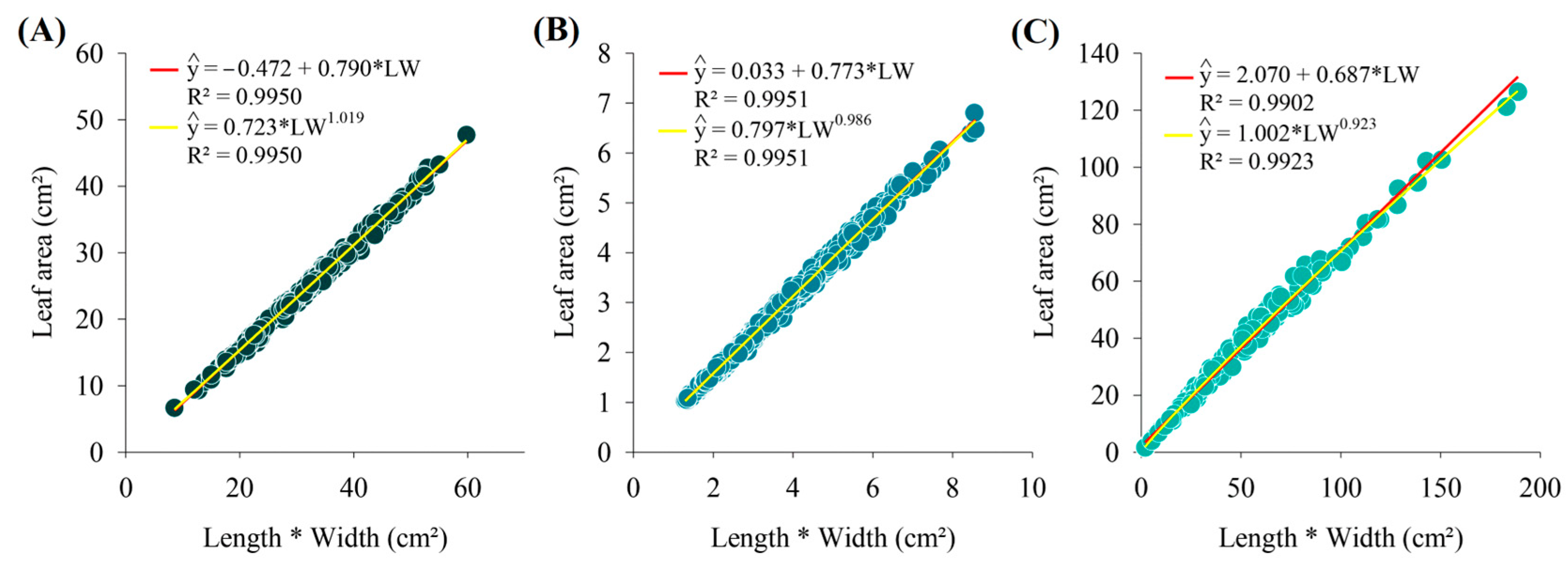
| 3 | Linear | 0.9950 | 0.9975 | 0.9987 | 0.266 | 0.516 | 0.406 | 0.0164 | |
| 4 | Power | 0.9108 | 0.9544 | 0.9763 | 4.769 | 2.184 | 1.751 | 0.0758 | |
| 5 | Power | 0.9153 | 0.9567 | 0.9776 | 4.532 | 2.129 | 1.676 | 0.0712 | |
| 6 | Power | 0.9950 | 0.9975 | 0.9987 | 0.265 | 0.515 | 0.405 | 0.0163 | |
| 7 | Exponential | 0.9077 | 0.9527 | 0.9750 | 4.946 | 2.224 | 1.762 | 0.0764 | |
| 8 | Exponential | 0.9147 | 0.9564 | 0.9770 | 4.567 | 2.137 | 1.662 | 0.0688 | |
| 9 | Exponential | 0.9147 | 0.9564 | 0.9770 | 4.567 | 2.137 | 1.662 | 0.0688 | |
| Libidibia ferrea | |||||||||
| 1 | Linear | 0.9146 | 0.9563 | 0.9772 | 0.103 | 0.322 | 0.250 | 0.1060 | |
| 2 | Linear | 0.9315 | 0.9651 | 0.9819 | 0.083 | 0.288 | 0.220 | 0.0892 | |
| 3 | Linear | 0.9951 | 0.9975 | 0.9987 | 0.005 | 0.077 | 0.058 | 0.0221 | |
| 4 | Power | 0.9314 | 0.9650 | 0.9820 | 0.083 | 0.288 | 0.216 | 0.0841 | |
| 5 | Power | 0.9331 | 0.9660 | 0.9822 | 0.081 | 0.285 | 0.216 | 0.0817 | |
| 6 | Power | 0.9951 | 0.9975 | 0.9987 | 0.005 | 0.076 | 0.058 | 0.0220 | |
| 7 | Exponential | 0.9254 | 0.9620 | 0.9799 | 0.090 | 0.301 | 0.219 | 0.0837 | |
| 8 | Exponential | 0.9113 | 0.9546 | 0.9753 | 0.108 | 0.329 | 0.256 | 0.0973 | |
| 9 | Exponential | 0.9113 | 0.9546 | 0.9753 | 0.108 | 0.329 | 0.256 | 0.0973 | |
| Tabebuia aurea | |||||||||
| 1 | Linear | 0.9223 | 0.9603 | 0.9794 | 43.190 | 6.572 | 4.958 | 0.6849 | |
| 2 | Linear | 0.8926 | 0.9447 | 0.9709 | 59.706 | 7.727 | 5.752 | 0.6037 | |
| 3 | Linear | 0.9902 | 0.9950 | 0.9975 | 5.459 | 2.336 | 1.856 | 0.0877 | |
| 4 | Power | 0.9424 | 0.9708 | 0.9850 | 32.011 | 5.657 | 4.375 | 0.1460 | |
| 5 | Power | 0.9394 | 0.9692 | 0.9838 | 33.837 | 5.817 | 4.241 | 0.1497 | |
| 6 | Power | 0.9923 | 0.9961 | 0.9980 | 4.295 | 2.072 | 1.591 | 0.0594 | |
| 7 | Exponential | 0.9167 | 0.9574 | 0.9758 | 48.088 | 6.934 | 5.655 | 0.2393 | |
| 8 | Exponential | 0.8973 | 0.9472 | 0.9677 | 61.331 | 7.831 | 6.408 | 0.2431 | |
| 9 | Exponential | 0.8973 | 0.9472 | 0.9677 | 61.331 | 7.831 | 6.408 | 0.2431 | |
Disclaimer/Publisher’s Note: The statements, opinions and data contained in all publications are solely those of the individual author(s) and contributor(s) and not of MDPI and/or the editor(s). MDPI and/or the editor(s) disclaim responsibility for any injury to people or property resulting from any ideas, methods, instructions or products referred to in the content. |
© 2025 by the authors. Licensee MDPI, Basel, Switzerland. This article is an open access article distributed under the terms and conditions of the Creative Commons Attribution (CC BY) license (https://creativecommons.org/licenses/by/4.0/).
Share and Cite
Silva, T.I.d.; Ribeiro, J.E.d.S.; Santos, T.S.d.; Correia, M.R.S.; Ribeiro, M.C.B.d.O.; Mendonça, A.J.T.; Silva, A.G.C.d.; Oliveira, P.H.d.A.; Coêlho, E.d.S.; Barros Júnior, A.P.; et al. Can a Non-Destructive Method Predict the Leaf Area of Species in the Caatinga Biome? Diversity 2025, 17, 234. https://doi.org/10.3390/d17040234
Silva TId, Ribeiro JEdS, Santos TSd, Correia MRS, Ribeiro MCBdO, Mendonça AJT, Silva AGCd, Oliveira PHdA, Coêlho EdS, Barros Júnior AP, et al. Can a Non-Destructive Method Predict the Leaf Area of Species in the Caatinga Biome? Diversity. 2025; 17(4):234. https://doi.org/10.3390/d17040234
Chicago/Turabian StyleSilva, Toshik Iarley da, João Everthon da Silva Ribeiro, Thainan Sipriano dos Santos, Marcos Roberto Santos Correia, Maria Carolina Borges de Oliveira Ribeiro, Allysson Jonhnny Torres Mendonça, Antonio Gideilson Correia da Silva, Pablo Henrique de Almeida Oliveira, Ester dos Santos Coêlho, Aurélio Paes Barros Júnior, and et al. 2025. "Can a Non-Destructive Method Predict the Leaf Area of Species in the Caatinga Biome?" Diversity 17, no. 4: 234. https://doi.org/10.3390/d17040234
APA StyleSilva, T. I. d., Ribeiro, J. E. d. S., Santos, T. S. d., Correia, M. R. S., Ribeiro, M. C. B. d. O., Mendonça, A. J. T., Silva, A. G. C. d., Oliveira, P. H. d. A., Coêlho, E. d. S., Barros Júnior, A. P., Silva, E. F. d., Rubio-Casal, A. E., de Lima, J. L. M. P., Silva, T. G. F. d., & Jardim, A. M. d. R. F. (2025). Can a Non-Destructive Method Predict the Leaf Area of Species in the Caatinga Biome? Diversity, 17(4), 234. https://doi.org/10.3390/d17040234