Article

Changes and Influencing Factors of Carbon Content in Surface Sediments of Different Sedimentary Environments Along the Jiangsu Coast, China

1
School of Marine Science and Engineering, Nanjing Normal University, Nanjing 210023, China
2
Jiangsu Key Laboratory of Ocean-Land Environmental Change and Ecological Construction, Nanjing Normal University, Nanjing 210023, China
*
Authors to whom correspondence should be addressed.
Diversity 2025, 17(3), 158; https://doi.org/10.3390/d17030158
Submission received: 31 December 2024 / Revised: 21 February 2025 / Accepted: 23 February 2025 / Published: 25 February 2025

Abstract

:
Coastal areas are essential for global ‘blue carbon’ burial, significantly impacting the global carbon cycle. To better understand the carbon burial capacity, impact factors, and response mechanisms of surface sediments in different coastline regions, this study investigated the surface sediments of the Spartina alterniflora vegetation, transition, and bare flat areas along Jiangsu coast in China. The results indicated significant changes in organic carbon (OC), inorganic carbon (IC), and various physicochemical property indicators between the three coastal environments. There were also significant differences in the important impact factors of OC and IC in each region. In areas of vegetation, OC and IC influenced each other, while nitrogen (N), clay, and sand were common impact factors. The pH only had a significant impact on OC. In the bare flat area, the important impact factors of OC and IC were identical: OC/IC, clay, salinity (SAL), and sand. However, the important impact factors of OC and IC in the transition area have undergone significant changes. The important impact factors of OC were N, total phosphorus (TP), total sulfur (TS), SAL, and sand. The partial least squares regression analysis results of IC were poor, and there were no important impact factors. This study refined the spatial distribution patterns and response mechanisms to the important impact factors of carbon in different coastal subregions, providing a basis for accurately evaluating the role of coastal wetlands in mitigating global climate change.

1. Introduction

Coastal areas are important sites for global ‘blue carbon’ burial, significantly impacting the global carbon cycle, which is crucial in mitigating global climate change [1,2]. Coastal areas have significant land–sea interactions [3,4,5,6] and unique spatiotemporal changes in salt marsh vegetation distribution, hydrodynamic processes, and geomorphic features [7]. Salt marsh vegetation is widely distributed in humid temperate to subtropical climates, typically occupying the upper silt–muddy intertidal zones. The presence of salt marsh vegetation profoundly alters local sedimentary environmental conditions. In vegetated salt marsh areas, plant growth reduces flow velocity, attenuates wave energy [8,9,10,11], and promotes sediment deposition and tidal flat accretion, thereby preventing surface erosion [12,13,14]. In contrast, bare flat areas without vegetation experience stronger hydrodynamic forces from currents and waves, making sediments more susceptible to erosion and transport [15,16,17]. Transitional areas between these areas demonstrate intermediate wave energy and wave height characteristics compared to vegetated and non-vegetated areas [8]. The difference in sedimentary environment conditions in different coastal areas will inevitably affect the efficiency of carbon burial in different parts of coastal areas. However, there is limited research on the carbon sequestration efficiency, main influencing factors, and response mechanisms in different sedimentary environments along the coast. This study aims to enhance the understanding of carbon storage capacity and key impact factors in coastal areas while providing a reference for accurately evaluating the status and role of coastal wetlands in global carbon cycling.
In the late 1970s, China’s Jiangsu Province introduced Spartina alterniflora from the United States to reduce wave impacts, strengthen embankments, encourage silt, and protect beaches. After approximately 40 years of growth, many S. alterniflora wetlands have developed in the coastal tidal flats of Jiangsu, and this has changed the original ‘bare flat’ attribute of the tidal flats and formed an obvious distribution pattern of S. alterniflora vegetation areas, transition areas, and bare flat areas. For the past few years, many studies have focused on the distribution pattern of organic carbon (OC) [18,19,20], sources of OC [21,22] in the coastal zone of Jiangsu, factors influencing carbon distribution in tidal flats [20,23,24], and the impact of S. alterniflora on coastal carbon sequestration [22,25,26,27,28,29]. However, there is little research on the distribution characteristics and important impact factors of inorganic carbon (IC) and OC content in different sedimentary environments. This study investigated S. alterniflora vegetation, transition, and bare flat areas at multiple transects along the Jiangsu coast by metering IC and OC content and the related physical and chemical properties of surface sediment to (1) reveal the change characteristics of various indicators of surface sediments in different sedimentary environments, (2) identify the important factors affecting the burial of OC and IC in vegetation, transition, and bare flat areas, and (3) analyze the response mechanisms of OC and IC burial in S. alterniflora vegetation, transition, and bare flat areas to the important impact factors.

2. Materials and Methods

2.1. Study Area

China is situated in the southeastern part of the Eurasian continent, characterized by high terrain in the west and lower elevations in the southeast. The western region features numerous mountains and plateaus, while the eastern coastal areas are dominated by hills and plains, forming a step-like descending slope that peaks at the Qinghai-Tibet Plateau in the southwest and gradually declines eastward. The Yangtze River and the Yellow River, the third and sixth longest rivers in the world, respectively, both originate from the Qinghai-Tibet Plateau and flow from west to east into the ocean. Jiangsu Province is in Eastern China. Under the influence of the Yellow, Huaihe, and Yangtze Rivers, a landform with low-lying terrain, numerous rivers and lakes, dense water networks, and plains has developed (Figure 1). The Jiangsu coast is a transitional zone between the Subei Plain in the west and the Yellow Sea in the east. It has a unique geographical location with a straight coastline. The sediment from the river flowing into the sea is redistributed under seawater, forming a silty and muddy coastline dominated by fine sand, silt, and clay. The tidal flats are extremely gentle, with an average slope of 0.2‰. A large number of S. alterniflora grows on the tidal flat, which changes the original sedimentary environment of the tidal flat and divides the tidal flat into vegetation area, transition area (0–300 m from the edge of the S. alterniflora wetland to the sea), and bare flat area (300 m beyond the edge of the S. alterniflora wetland to the sea). The seawater transport capacity is weak in the S. alterniflora growing area. While the influence of S. Alterniflora is weakened in the transition area, and the seawater transport capacity is increased, the bare flat area is far away from the S. alterniflora growing area, and the seawater transport capacity is stronger. The land near the coast grows Phragmites australis, Imperata cylindrica, Suaeda glauca, and other plants. Jiangsu belongs to the East Asian monsoon climate zone, located in the transition zone between warm temperate and subtropical zones, with a warm and humid climate and four distinct seasons: cold winters and hot summers, rainy and hot seasons, abundant rainfall, and concentrated rainfall.

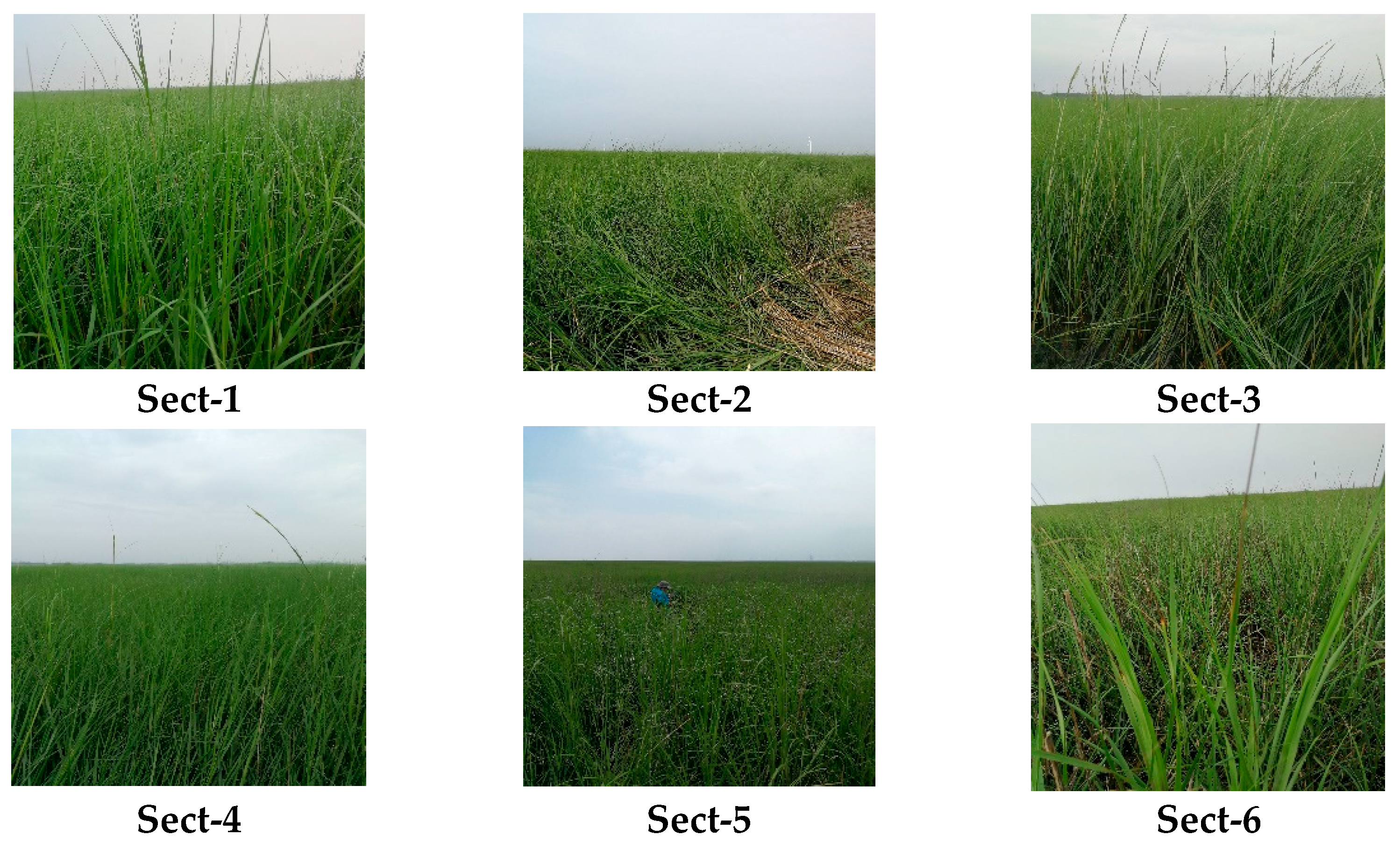
2.2. Sample Collection

In July 2022, a field investigation was carried out on the coast of Jiangsu Province. According to the research objectives and the topography of tidal flats, six representative sampling transects with S. alterniflora in Sheyang Port (Sect-1), Huangshagang (Sect-2, Sect-3), Dongtai Estuary (Sect-4), Dulonggang (Sect-5), and Xiaoyangkou Town (Sect-6) were finally selected (Figure 1 and Figure 2). Stainless-steel sampling shovels were used to collect surface sediment samples (0–3 cm) from the vegetation area (S. alterniflora), transition area, and the bare flat area at intervals of 30–60 m in each transect. Then, 114 surface sediment samples were collected from the 6 transects (33 surface sediment samples from S. alterniflora wetland, 37 surface sediment samples from the transition area, and 44 surface sediment samples from the bare flat area). The collected samples were refrigerated and transported to the laboratory for sample pretreatment and experimentation. Samples were tested for sediment particle size, total carbon (TC), OC, nitrogen (N), pH, salinity (SAL), total phosphorus (TP), and total sulfur (TS).

2.3. Laboratory Analyses

The initial pretreatment process for samples used for carbon content (TC and OC), pH, SAL, TP, and TS testing was the same. Approximately 15 g of the sediment sample was weighed and freeze-dried at −60 °C. It was ground in an agate mortar and passed through a 200-mesh fine sieve. The ground sample was divided into three parts: one for measuring TC, TP, and TS, one for measuring pH and SAL, and one for further processing to measure OC.
TC content analysis was performed by directly weighing the low-temperature freeze-dried and ground samples. Samples for OC content analysis also needed to be further processed into freeze-dried and ground samples. Then, 2 g of the low-temperature freeze-dried and ground samples was weighed and put in a 50 mL centrifuge tube, 10 mL of 10% hydrochloric acid was added to take IC away from the sample, and then ultra-pure water was added to dilute. The sample was then centrifuged to remove the supernatant, which was repeated multiple times until the solution was nearly neutral. It was then dried at low temperature, ground finely, and weighed for measurement. The OC and TC contents were measured using the Vario MAX element analyzer (Elementar Co, Hesse-Darmstadt, Germany) with a test error of less than 0.5%. As IC was removed from the sample to measure OC, the OC content measured by the instrument was larger than the OC content in the natural sample. To eliminate this error, a simple mathematical method can correct the results and obtain the true OC result (Equation (1)). The IC content result can be obtained by subtracting the actual OC content from the total carbon content (Equation (2)):
OC T = O C M × 1 T C × 1 O C T 1 ,
IC = TC OC T ,
where OC T is the actual organic carbon content (%), O C M is the measured organic carbon content (%) after removing IC, TC is the measured total carbon content, and IC is the inorganic carbon content (%).
Then, 5 g of freeze-dried and ground samples were weighed and pressed into pellets under 30 tons of high pressure using boric acid. After sample preparation, the TP and TS contents were measured using an X-ray fluorescence element analyzer (PANalytical Co. Almelo, The Netherlands), with a less than 5% measurement error.
To measure pH and SAL, 2.5 g of the freeze-dried and ground sample was put into a 10 mL test tube before ultra-pure water was added at a sediment:water ratio of 1:2.5. The test tube was covered with the lid, shaken thoroughly to mix the sediment and water, and then placed on the test tube rack for 3 min. An SX751 multi-parameter water quality meter (Sanxin Instrument Co., Shanghai, China) was used to determine pH and SAL levels. The probe was submerged in water during the measurement, a reading was taken three times, and the average value was calculated.
Approximately 1 g of sediment was separated and placed in a 100 mL glass beaker, followed by adding 10 mL of 10% hydrogen peroxide to eliminate organic matter from the sample. Subsequently, 5 mL of diluted hydrochloric acid was added to remove the calcium cementing material in the sample. The mixture was then diluted with ultra-pure water and allowed to stand for 24 h before siphoning off the supernatant. We repeated this process multiple times until the solution was nearly neutral. Sodium hexametaphosphate was introduced to disperse the sample, which was subjected to ultrasonic agitation using a shaker. Finally, particle size measurements were conducted using a Mastersizer 3000 laser particle size analyzer (Malvern Co., Malvern, UK). The analytical error of the instrument was less than 2%.

2.4. Research Methods and Data Processing

All experimental data were statistically analyzed to obtain the maximum, minimum, and average values. The coefficient of variation (CV) and other indicators reflecting the data distribution characteristics and basic composition were also obtained. Box plots were used to display the dispersion of the data, and comparisons between multiple sets of data were used to show the differences in the indicators in each area.
The partial least squares regression (PLSR) method [30] was employed to identify the important impact factors of IC and OC in the vegetation, transition, and bare flat areas. The PLSR method is a linear multivariate model associating two data matrices (X and Y). This model combines the advantages of principal components, canonical correlation, and linear regression analyses, while effectively addressing multicollinearity issues between variables [31]. The PLSR method has been proven to determine the significance of impact factors [20,32,33]. The importance of independent variables was measured by the variable importance in projection (VIP) value [34], and the action direction of the independent variables was represented by regression coefficients (RCs) [35]. R2 and Q2 express the model’s explanatory ability and predictive ability, and the closer R2 and Q2 are to 1, the stronger the explanatory ability and predictive ability [34].
The data analysis was conducted using Excel 2016, GRAPHER 11, and SIMCA14.1 software packages.

3. Results

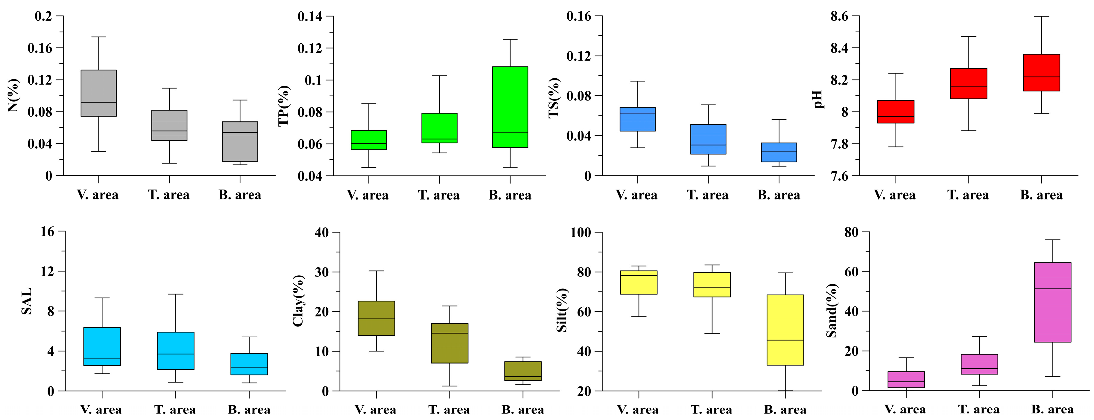
3.1. Change Characteristics of Physicochemical Properties of Surface Sediments

In the sampling section, all indicators showed significant changes in vegetation, transition, and bare flat areas (Figure 3 and Table 1). The N content of surface sediment in the vegetation area ranged from 0.03 to 0.44%, with an average of 0.11%; in the transition area, it ranged from 0.02 to 0.11%, with an average of 0.06%; in the bare flat area, it ranged from 0.01 to 0.09%, with an average of 0.05%. The average N content gradually decreased from the vegetation area to the transition and bare flat areas. Still, the CV was relatively large across different regions, indicating high data dispersion. The TP content of surface sediments in the vegetation area ranged from 0.05 to 0.09%, with an average of 0.06; in the transition area, it ranged from 0.05 to 0.13%, with an average of 0.07%; in bare flat areas, it ranged from 0.05 to 0.13%, with an average of 0.08%. The CV and the average TP content gradually increased from the vegetation area to the transition and bare flat area. The TS content of surface sediments in the vegetation area ranged from 0.03 to 0.14%, with an average value of 0.06%; in the transitional area, it ranged from 0.01 to 0.07%, with an average value of 0.04%; in the bare flat area, it ranged from 0.01% to 0.06%, with an average value of 0.03%. The mean TS content gradually decreased from the vegetation area to the transitional and bare flat areas, and the CV gradually increased. The pH value of surface sediment in the vegetation area ranged from 7.70 to 8.24, with an average value of 7.98; in the transition area, it ranged from 7.88 to 8.59, with an average value of 8.16; in the bare flat area, it ranged from 7.99 to 8.60, with an average value of 8.20. The average pH value gradually increased from the vegetation area to the transition and bare flats areas, and the CV remained very small. The SAL values of surface sediments in the vegetation area ranged from 1.71 to 14.40 g/kg, with an average value of 4.52 g/kg; in the transition area, they ranged from 0.88 to 21 g/kg, with an average value of 4.74 g/kg; in the bare flat area, they ranged from 0.81 to 8.82 g/kg, with an average value of 2.97 g/kg. The average SAL value gradually decreased from the vegetation area to the transition and bare flats area, with a large CV and scattered data. The clay, silt, and sand content, which reflect the grain size of the sediment, also showed regular changes between the three regions. The average values of clay and silt in the vegetation area were the highest, and the average values of sand were the lowest, at 18.95%, 74.87%, and 6.23%, respectively. The clay, silt, and sand contents in the transition area were at a medium level, at 12.53%, 69.97%, and 17.50%, respectively. The average values of clay and silt in bare flat areas were lowest, and the average values of sand were highest, at 5.73%, 49.07%, and 45.17%, respectively. The CVs of clay and silt gradually increased from the vegetation area to the transition and bare flat areas, and the CV of sand gradually decreased from the vegetation area to the transition and bare flat areas.

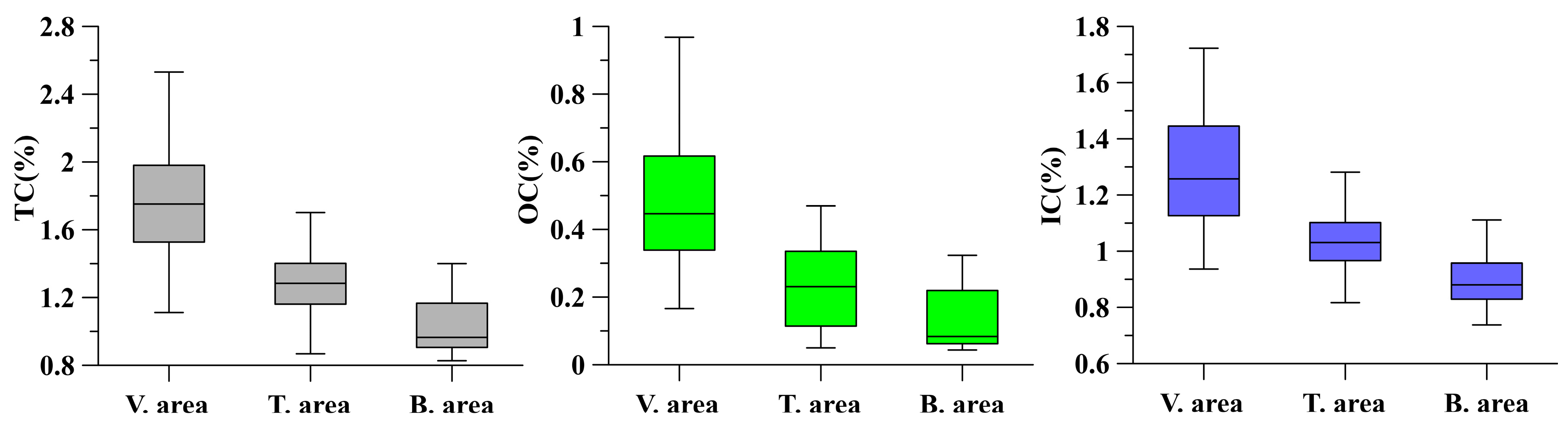
3.2. Variation Characteristics of OC and IC Content in Surface Sediments

These transects’ TC, OC, IC, and CV contents showed regular changes (Figure 4 and Table 1). In the vegetation area, the content of TC ranged from 1.11 to 2.53%, the average value was 1.77%, and CV was 21.14. In the transition zone, the content of TC ranged from 0.87 to 1.86%, with an average of 1.29% and a CV of 18.98. In the bare flat area, the content of TC ranged from 0.83 to 1.40%, the average value was 1.02%, and the CV was 15.76. The mean value of TC and CV decreased gradually from the vegetation area to the transition and bare flat area. In the vegetation area, OC content ranged from 0.17 to 0.97%, with an average value of 0.47% and a CV of 39.72. In the transitional area, OC content ranged from 0.05 to 0.47%, with an average value of 0.24% and a CV of 51.21. In the bare flat area, OC content ranged from 0.04 to 0.32%, with an average value of 0.12% and a CV of 71.19. The mean value of OC decreased gradually, whereas the CV increased gradually from the vegetation area to the transition and bare flat areas. In the vegetation area, IC content ranged from 0.94 to 1.727%, with an average value of 1.29% and a CV of 16.73. In the transitional area, IC content ranged from 0.82 to 1.64%, with an average value of 1.06% and a CV of 15.15. In the bare flat area, IC content ranged from 0.74 to 1.11%, with an average value of 0.90% and a CV of 9.64. The CV and the mean value of IC decreased gradually from the vegetation area to the transition and bare flat areas. The data also showed that the IC content was much higher than the OC across all three areas.

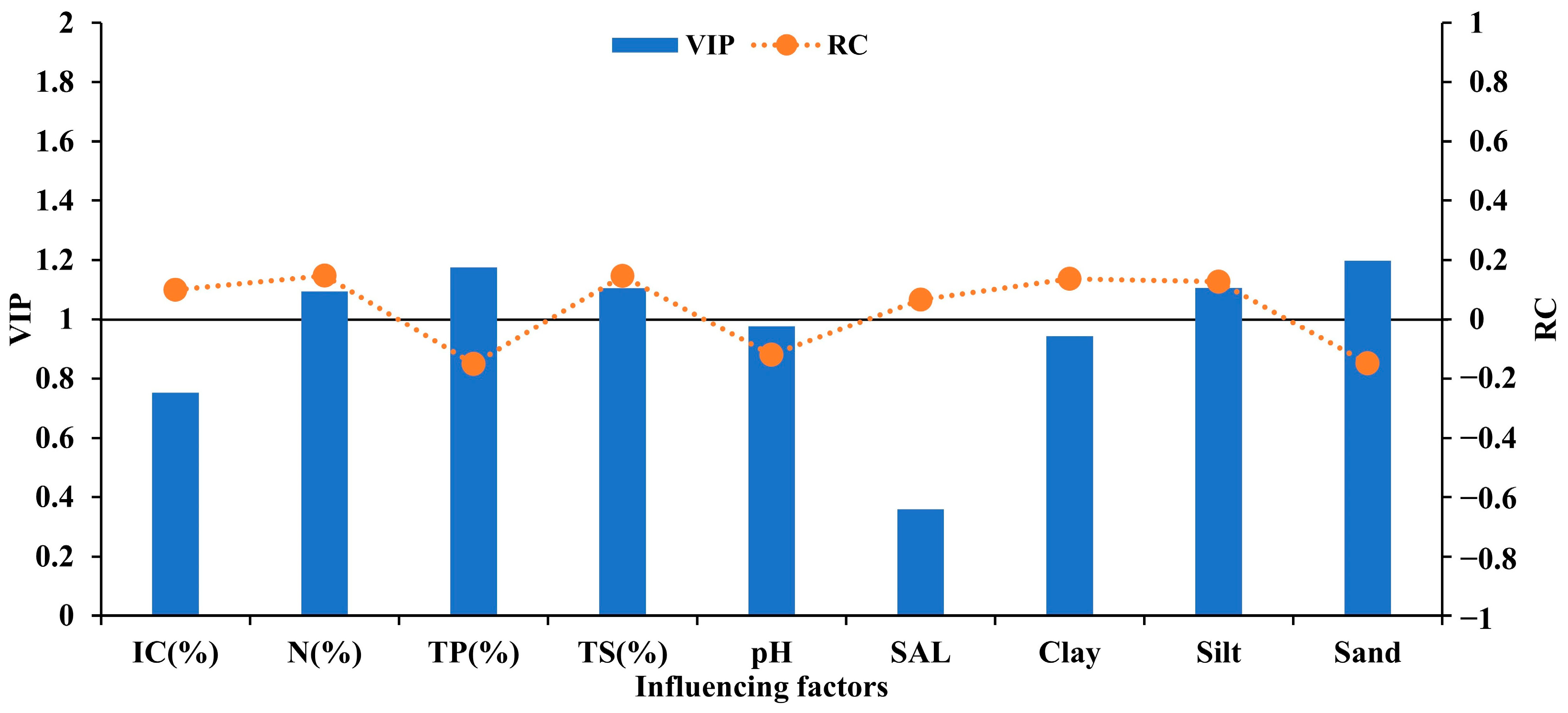
3.3. Identification of the Importance of Factors Affecting IC and OC

The PLSR model was used to analyze all sample data across the different areas to identify important factors affecting the spatial distribution of IC and OC content.
In the vegetation area, OC was used as the dependent variable, and IC, N, TP, TS, pH, SAL, clay, silt, and sand were used as independent variables for the PLSR analysis. The results showed that the best forecast accuracy of OC could be obtained by extracting one principal component (Table 2), with an R2 of 0.6421, demonstrating that the selected independent variables had good results on the impact factors of OC. The maximum Q2 value was 0.5797, indicating that the model displayed a good fit. The importance of impact factors on OC content can be ranked as follows: sand (VIP = 1.39) > IC (VIP = 1.29) > N (VIP = 1.24) > clay (VIP = 1.18) > pH (VIP = 1.01) > TP (VIP = 0.87) > TS (VIP = 0.67) > SAL (VIP = 0.49) > silt (VIP = 0.08), in which the VIP values of sand, IC, N, clay, and pH were greater than 1, which were important impact factors of OC content. The RC values of IC, N, TS, SAL, and clay were positive and positively impacted the OC content. The RC values of TP, pH, silt, and sand were negative and adversely impacted the OC content (Figure 5a). IC was used as a dependent variable. OC, N, TP, TS, pH, SAL, clay, silt, and sand were independent variables for the PLSR analysis. The results showed that the optimal forecast accuracy of IC could be obtained by extracting four principal components (Table 2). The R2 value reached 0.8037, indicating that the prediction results of the selected independent variables were good, and the maximum Q2 value was 0.7124, showing that the fitting degree of the prediction model was also good. The importance scores of IC content were as follows: OC (VIP = 1.73) > sand (VIP = 1.53) > clay (VIP = 1.12) > N (VIP = 1.02) > TS (VIP = 0.83) > pH (VIP = 0.65) > TP VIP = (0.38) > silt (VIP = 0.26) > SAL (VIP = 0.14), where OC, sand, clay, and N (with a VIP value greater than 1) were important impact factors for IC content. The RC values of OC, N, TP, TS, pH, and clay were positive and positively affected IC content. The RC values of SAL, silt, and sand were negative, which had a negative impact on IC content (Figure 5b).
In the transition area, OC was used as the dependent variable and IC, N, TP, TS, pH, SAL, clay, silt, and sand were used as independent variables for the PLSR model analysis. The results showed that the optimal forecast accuracy of OC could be obtained by extracting one principal component (Table 3). The R2 value was 0.7941, indicating that the selected independent variables had good prediction results. The maximum Q2 value was 0.7724, demonstrating that the PLSR model fit well. The importance of the factors influencing OC content was ranked as follows: sand (VIP = 1.20) > TP (VIP = 1.18) > silt (VIP = 1.11) > TS (VIP = 1.11) > N (VIP = 1.09) > pH (VIP = 0.98) > clay (VIP = 0.94) > IC (VIP = 0.75) > SAL (VIP = 0.36), in which the VIP values of sand, TP, TS, and N were greater than 1, meaning they were important impact factors for OC content. The RC values of IC, N, TS, SAL, clay, and silt were positive and positively impacted the OC content. The RC values of TP, pH, and sand were negative, which had a negative impact on OC content (Figure 6). IC was used as a dependent variable. OC, N, TP, TS, pH, SAL, clay, silt, and sand were independent variables for the PLSR model analysis. The results showed that the optimal forecast accuracy of IC could be obtained by extracting two principal components (Table 3). However, the R2 value reached 0.3800, demonstrating that the prediction results of the selected independent variables were not ideal. The maximum Q2 value was only 0.2715, indicating that the degree of fit of the model was also poor.
In the bare flat area, PLSR analysis was performed with OC as the dependent variable and IC, N, TP, TS, pH, SAL, clay, salt, and sand as independent variables. The results showed that extracting two principal components obtained the best OC forecast accuracy (Table 4). The R2 value was 0.9057, demonstrating that the prediction results of the selected independent variables were excellent, with a maximum Q2 value of 0.8886, demonstrating an optimal fitting degree for the model. The importance of the factors influencing OC content was as follows: sand (VIP = 1.33) > clay (VIP = 1.30) > silt (VIP = 1.26) > IC (VIP = 1.17) > N (VIP = 0.83) > TS (VIP = 0.77) > TP (VIP = 0.77) > pH (VIP = 0.62) > SAL (VIP = 0.58). The VIP values of sand, clay, silt, and IC, which are important impact factors of OC content, were greater than 1. The RC values of IC, N, TS, SAL, clay, and silt were positive, which resulted in a positive effect on the OC content. The RC values of TP, pH, and sand were negative, which negatively impacted the OC content (Figure 7a). IC was used as the dependent variable. OC, N, TP, TS, pH, SAL, clay, silt, and sand were independent variables for the PLSR model analysis. The results showed that the best forecast accuracy of IC could be obtained by extracting two principal components (Table 4). The R2 value reached 0.8339, demonstrating that the prediction results of the selected independent variables were good, and the maximum Q2 value reached 0.7985, demonstrating that the fitting degree of the PLSR model was also good. Scores for the importance of IC content were as follows: sand (VIP = 1.51) > silt (VIP = 1.44) > clay (VIP = 1.41) > OC (VIP = 1.33) > SAL (VIP = 0.89) > N (VIP = 0.20) > TS (VIP = 0.18) > TP (VIP = 0.10) > pH (VIP = 0.05). OC, sand, silt, and clay, with VIP values greater than 1, were important impact factors of IC content. The RC values of OC, TP, pH, SAL, silt, and clay were positive and positively impacted the IC content. The RC values of N, TS, and sand were negative, affecting the IC content (Figure 7b).

4. Discussion

4.1. Discussion on the Reasons for the Changes in Various Indicators

The N content gradually decreased from the vegetation to the transition and bare flat areas, primarily due to the nature of N. Previous studies have indicated a close relationship between N and OC [36,37], both of which are vital components of organic matter. The vegetation area had the highest OC content, whereas the bare flat area had the lowest OC content, leading to a similar trend in N distribution. The gradual decrease in TS content from vegetation to bare flats can be attributed to S. alterniflora growth, which is significantly enriched in sulfur [38,39,40,41]. This explains why the TS content decreased with the increasing distance from S. alterniflora. Phosphorus plays an essential role in plant growth. Some phosphorus present in sediments within the vegetation area was consumed by plant growth, resulting in a lower TP content compared to bare flat areas. The pH value was lowest in the vegetation area and highest in the bare flat area, and this may be related to the release of organic acids during the growth of S. alterniflora, which can reduce the pH of sediments [42,43]. The SAL gradually decreased from the vegetation area to the transition and bare flat areas, possibly related to organisms’ tidal action and salt retention capacity [20]. Changes in sediment particle composition (clay, silt, and sand) were mainly affected by hydrodynamic conditions. In the coastal vegetation area, the coast and vegetation obstruction weakened the carrying capacity of seawater, and finer sediment particles were deposited. However, in the bare flat area, which is relatively far from the coast and vegetation, stronger hydrodynamic conditions transported larger particles for deposition, consistent with existing regional research [20].

4.2. Response Mechanism of Organic/Inorganic Carbon Burial in the Vegetation Area to Important Impact Factors

There was a good correlation between OC and IC in vegetated areas (Table 5), indicating similar impact factors. It can be seen from Figure 4 that the important impact factors of IC and OC in the vegetated area were essentially the same. The OC and IC were important impact factors for each other. Owing to the growth of dense S. alterniflora in the vegetation area, IC brought about by seawater was easily deposited owing to the weakened transport capacity, resulting in the highest IC content in the vegetation area. Simultaneously, vegetation growth has led to the precipitation of more OC. OC and IC had high values in vegetated areas and were important impact factors. N, clay, and sand significantly affected both IC and OC. As an important nutrient element, N can stimulate plant growth and increase the enrichment of OC [44], and more than 90% of N exists in the form of organic combinations in sediments [45]. At the same time, the denser the plants grow, the more conducive they are to weakening the hydrodynamic forces and enriching the IC brought about by seawater. The increase in clay and decrease in sand are the direct results of the impact of vegetation on seawater dynamics. Fine particles have larger specific surface areas and can adsorb more OC. The sediment composed of fine particles has poor water permeability, which reduces OC’s decomposition ability, weakens the sediment’s respiration process, and increases the content of OC in the sediment [46]. Sand has poor water-holding and carbon adsorption capacities, which is not conducive to carbon enrichment [47]. In vegetated areas, reducing sand content is beneficial to the enrichment of carbon, so the amount of sand content would also significantly affect the change in carbon content. The ‘particle size effect’ [38] was significant in vegetation areas. The pH was an important factor influencing OC (but not IC) and was related to the factors affecting pH changes in the vegetation area. In the growth zone of S. alterniflora, releasing organic acids can reduce the pH [42,43]. Lower pH deposits generally carry more positive charges, which is beneficial to the sorption of negatively charged OC [48]. The change in pH is generally unrelated to IC, but a lower pH may lead to the decomposition of IC [49,50], and this means pH is not an important impact factor for IC in vegetation areas.

4.3. Response Mechanism of Organic/Inorganic Carbon Burial in the Transition Area to Important Impact Factors

In the transitional zone, the correlation between OC and IC was significantly reduced (Table 5), indicating that the factors impacting IC and OC in this region should also be relatively different. The PLSR analysis results showed that in the transition zone, the important impact factors of OC were N, TP, TS, silt, and sand (Figure 5), and the cumulative interpretation rate and fitting degree of the PLSR analysis results for IC were poor (Table 3). Therefore, discussing the important impact factors of IC in the transition area is meaningless. N, an important factor affecting OC enrichment in vegetation areas, will continue to affect OC enrichment because the transition area is close to the vegetation area. Still, its importance decreased (the VIP value decreased from 1.24 to 1.09). Phosphorus and sulfur are two nutrient elements required for plant growth; however, in the S. alterniflora growth area, TP decreased due to plant growth consumption, and TS increased due to the sulfur enrichment ability of S. alterniflora [38,39,40,41]. Therefore, TS and TP in the S. alterniflora growth area responded to this opposite change rather than influencing OC content. However, in the transition area, TP and TS were important impact factors for OC due to the reduction in phosphorus consumption and the weakening of the sulfur enrichment effect. After leaving the vegetation area, vegetation’s wave energy dissipation effect weakened, and seawater’s carrying capacity was enhanced, decreasing the clay content of fine particles and increasing the silt and sand content of coarse particles in sediments. Because the adsorption capacity of silt and sand for OC was not as strong as that of clay, the content of OC in sediments decreased. Silt and sand have large particles, and with an increase in their content, the ventilation and water permeability of the sediment increased, which can strengthen the breathing process of the sediment, and the amount of decomposed OC may increase. Therefore, an increase in silt and sand content led to a decline in the OC content of the surface sediment, which is an important factor influencing OC enrichment in the transition area.

4.4. Response Mechanism of Organic/Inorganic Carbon Burial to Important Impact Factors in the Bare Flat Area

In the bare flat area, the correlation between OC and IC increased again, reaching a good correlation (Table 5), which indicated that they had similar enrichment mechanisms and should have similar impact factors. The results of the PLSR analysis showed that the forecast accuracy and fitting degree of OC and IC were good (Table 4) and had the same important impact factors. OC, IC, clay, silt, and sand were important factors that impacted OC and IC in bare flats (Figure 6). Because the bare flat area is far from the vegetation area, sediment deposition was less affected by vegetation and the coast. It was mainly affected by the dynamic conditions of seawater. The hydrodynamics of the bare flat areas were the largest among the three regions, resulting in the maximum annual average sand content and the minimum average clay content. The ‘particle size effect’ of sediment particles on carbon was the most significant [38], and the sediment components were both important impact factors of OC and IC. Some played a positive role (fine-grained clay and silt), whereas others played a restraining role (coarse-grained sand). In tidal flat systems, both OC and IC were easily enriched in fine particles [20], and a good coupling relationship promoted their enrichment.

5. Conclusions

This study divided the Jiangsu coast into S. alterniflora vegetation, transition, and bare flat areas. The spatial differentiation of OC, IC, and various physicochemical properties of surface sediments and the important impact factors and response mechanisms of OC and IC in S. alterniflora vegetation, transition, and bare flat areas were studied. The results showed that OC, IC, N, TS, SAL, clay, and silt decreased from the S. alterniflora vegetation area to the transition and bare flat areas. At the same time, TP, pH, and sand increased from the S. alterniflora vegetation area to the transition and bare flat areas. The important impact factors of IC and OC also showed significant changes across each area. In the S. alterniflora vegetation areas, IC and OC were important impact factors, and N, clay, and sand were their common impact factors—only pH significantly affected OC. In the transition area, the PLSR analysis results of OC were ideal, and the important impact factors were N, TP, TS, silt, and sand. The PLSR analysis results of IC were poor, so it was difficult to explore the important impact factors of IC. In the bare flat area, OC and IC had the same important impact factors: OC/IC, clay, silt, and sand. In summary, grain size is an important factor that impacts carbon burial in different coastal regions.
Studying the physical and chemical properties of sediments in different coastal areas and the important influencing factors of carbon burial is beneficial for refining people’s understanding of the carbon burial capacity and contribution of different coastal areas. It can make people realize that increasing vegetation coverage in coastal tidal flats can not only sequester carbon through vegetation but also increase the accumulation of OC and IC in sediments, greatly improving the storage of coastal blue carbon and reducing the carbon dioxide content in the atmosphere, thereby slowing down the global warming. This also provides a basis for correctly evaluating the role and status of coastal areas in mitigating global climate change.

Author Contributions

Writing—original draft, data curation, visualization, investigation, software, L.X.; data curation, methodology, investigation, software, H.Y.; investigation, software, J.Y.; software, methodology, investigation, data curation, formal analysis, supervision, funding acquisition, conceptualization, Q.S.; data curation, investigation, Y.F. All authors have read and agreed to the published version of the manuscript.

Funding

This research received no external funding.

Institutional Review Board Statement

Not applicable.

Data Availability Statement

Data will be made available upon request.

Conflicts of Interest

The authors declare no conflicts of interest.

References

  1. Bai, J.; Zhang, G.; Zhao, Q.; Lu, J.; Cui, B.; Liu, X. Depth-distribution patterns and control of soil organic carbon in coastal salt marshes with different plant covers. Sci. Rep. 2016, 6, 34835. [Google Scholar] [CrossRef]
  2. Duarte, C.M.; Middelburg, J.; Caraco, N. Major role of marine vegetation on the oceanic carbon cycle. Biogeosciences 2005, 2, 1–8. [Google Scholar] [CrossRef]
  3. Pernetta, J.C.; Milliman, J.D. Land-Ocean Interactions in the Coastal Zone—Implementation Plan; IGBP Global Change Report No. 33. 215; International Geosphere-Biosphere Programme: Stockholm, Sweden, 1995. [Google Scholar]
  4. Shen, M. Review of “Sustainable development in east china sea evolution of resources and environment in coastal zone and bay area”. Geogr. Res. 2020, 39, 2427–2428. [Google Scholar]
  5. Shen, H.; Zhu, J. The land and ocean interactions in the coastal zone of china. Mar. Sci. Bull. 1999, 18, 11–17, (In Chinese with English abstract). [Google Scholar]
  6. Shu, Q.; Zhao, Y.; Hu, Z.; Yang, P.; Liu, Y.; Chen, Y.; Zhao, Z.; Zhang, M. Multi-proxy reconstruction of the Holocene transition from a transgressive to regressive coastal evolution in the northern Jiangsu Plain, East China. Palaeogeogr. Palaeoclimatol. Palaeoecol. 2021, 572, 110405. [Google Scholar] [CrossRef]
  7. Dussaillant, A.; Galdames, P.; Sun, C.L. Water level fluctuations in a coastal lagoon: El Yali Ramsar wetland, Chile. Desalination 2009, 246, 202–214. [Google Scholar] [CrossRef]
  8. Möller, I.; Spencer, T.; French, J.R.; Leggett, J.; Dixon, M. Wave Transformation Over Salt Marshes: A Field and Numerical Modelling Study from North Norfolk, England. Estuar. Coast. Shelf Sci. 1999, 49, 411–426. [Google Scholar] [CrossRef]
  9. Bouma, T.J.; Vries, M.B.D.; Low, E.; Kusters, L.; Herman, P.M.J.; Tánczos, I.C.; Temmerman, S.; Hesselink, A.; Meire, P.; Regenmortel, S.V. Flow hydrodynamics on a mudflat and in salt marsh vegetation: Identifying general relationships for habitat characterisations. Hydrobiologia 2005, 540, 259–274. [Google Scholar] [CrossRef]
  10. Schoutens, K.; Heuner, M.; Minden, V.; Ostermann, T.S.; Silinski, A.; Belliard, J.P.; Temmerman, S. How effective are tidal marshes as nature-based shoreline protection throughout seasons? Limnol. Oceanogr. 2019, 64, 1750–1762. [Google Scholar] [CrossRef]
  11. Neumeier, U. Velocity and turbulence variations at the edge of saltmarshes. Cont. Shelf Res. 2007, 27, 1046–1059. [Google Scholar] [CrossRef]
  12. Carling, P.A. Temporal and spatial variation in intertidal sedimentation rates. Sedimentology 1982, 29, 17–23. [Google Scholar] [CrossRef]
  13. French, J.R.; Spencer, T.; Murray, A.L.; Arnold, N.S. Geostatistical analysis of sediment deposition in two small tidal wetlands, Norfolk, UK. J. Coast. Res. 1995, 11, 308–321. [Google Scholar]
  14. Reed, D.J.; Spencer, T.; Murray, A.L.; French, J.R.; Leonard, L. Marsh surface sediment deposition and the role of tidal creeks: Implications for created and managed coastal marshes. J. Coast. Conserv. 1999, 5, 81–90. [Google Scholar] [CrossRef]
  15. Allen, J.R.L.; Duffy, M.J. Medium-term sedimentation on high intertidal mudflats and salt marshes in the Severn Estuary, SW Britain: The role of wind and tide. Mar. Geol. 1998, 150, 1–27. [Google Scholar] [CrossRef]
  16. Black, K.S.; Paterson, D.M.; Cramp, A. Sedimentary Processes in the Intertidal Zone; Geological Society Special Publication; Geological Society: London, UK, 1998. [Google Scholar]
  17. Li, H.; Yang, S. A review of influences of saltmarsh vegetation on physical processes in intertidal wetlands. Adv. Earth Sci. 2007, 6, 583–592, (In Chinese with English Abstract). [Google Scholar]
  18. Gao, J.; Bai, F.; Yang, G.; Ou, W. Distribution characteristics of organic carbon, nitrogen, and phosphor in sediments from different ecologic zones of tidal flats in north Jiangsu province. Quat. Sci. 2007, 27, 756–765, (In Chinese with English abstract). [Google Scholar]
  19. Zhang, H.; Yin, A.; Yang, X.; Wu, P.; Fan, M.; Wu, J.; Zhang, M.; Gao, C. Changes in surface soil organic/inorganic carbon concentrations and their driving forces in reclaimed coastal tidal flats. Geoderma 2019, 352, 150–159. [Google Scholar] [CrossRef]
  20. Yang, P.; Shu, Q.; Liu, Q.; Hu, Z.; Zhang, S.; Ma, Y. Distribution and factors influencing organic and inorganic carbon in surface sediments of tidal flats in northern Jiangsu, China. Ecol. Indic. 2021, 126, 107633. [Google Scholar] [CrossRef]
  21. Mao, Y.; Ma, Q.; Lin, J.; Chen, Y.; Shu, Q. Distribution and Sources of Organic Carbon in Surface Intertidal Sediments of the Rudong Coast, Jiangsu Province, China. J. Mar. Sci. Eng. 2021, 9, 992. [Google Scholar] [CrossRef]
  22. Liu, J.; Deng, D.; Zou, C.; Han, R.; Xin, Y.; Shu, Z.; Zhang, L. Spartina alterniflora saltmarsh soil organic carbon properties and sources in coastal wetlands. J. Soils Sediments 2021, 21, 3342–3351. [Google Scholar] [CrossRef]
  23. Li, T.; Zhang, G.; Wang, S.; Mao, C.; Tang, Z.; Rao, W. The isotopic composition of organic carbon, nitrogen and provenance of organic matter in surface sediment from the Jiangsu tidal flat, southwestern Yellow Sea. Mar. Pollut. Bull. 2022, 182, 114010. [Google Scholar] [CrossRef] [PubMed]
  24. Gong, Z.; Wen, T.; Jin, C.; Zhao, K.; Su, M. Distribution characteristics and influencing factors of soil organic carbon in tidal flat wetland of central Jiangsu, China. Chin. J. Appl. Ecol. 2023, 34, 2978–2984, (In Chinese with English Abstract). [Google Scholar]
  25. Zhang, G.; Bai, J.; Zhao, Q.; Jia, J.; Wang, X.; Wang, W.; Wang, X. Soil carbon storage and carbon sources under different Spartina alterniflora invasion periods in a salt marsh ecosystem. Catena 2021, 196, 104831. [Google Scholar] [CrossRef]
  26. Zhang, X.; Zhang, Z.; Li, Z.; Li, M.; Wu, H.; Jiang, M. Impacts of Spartina alterniflora invasion on soil carbon contents and stability in the Yellow River Delta, China. Sci. Total Environ. 2021, 775, 145188. [Google Scholar]
  27. Xu, X.; Wei, S.; Chen, H.; Li, B.; Nie, M. Effects of Spartina invasion on the soil organic carbon content in salt marsh and mangrove ecosystems in China. J. Appl. Ecol. 2022, 59, 1937–1946. [Google Scholar] [CrossRef]
  28. Sheng, Y.; Luan, Z.; Yan, D.; Li, J.; Xie, S.; Liu, Y.; Chen, L.; Li, M.; Wu, C. Effects of Spartina alterniflora Invasion on Soil Carbon, Nitrogen and Phosphorus in Yancheng Coastal Wetlands. Land 2022, 11, 2218. [Google Scholar] [CrossRef]
  29. Ding, X.; Wang, W.; Wen, J.; Feng, T.; Peñuelas, J.; Sardans, J.; Liang, C. Spartina alterniflora invasion differentially alters microbial residues and their contribution to soil organic C in coastal marsh and mangrove wetlands. Catena 2023, 230, 107246. [Google Scholar] [CrossRef]
  30. Wold, H. Soft modelling, the basic design and some extensions. In Systems Under Indirect Observation: Causality-StructurePrediction; Wold, H., Jöreskog, K.G., Eds.; North-Holland Publishing Company: Amsterdam, The Netherlands, 1982; Part II; pp. 1–54. [Google Scholar]
  31. Wold, S.; Sjöström, M.; Eriksson, L. PLS-regression: A basic tool of chemometrics. Chemom. Intell. Lab. Syst. 2001, 58, 109–130. [Google Scholar] [CrossRef]
  32. Fang, N.; Shi, Z.; Chen, F.; Wang, Y. Partial Least Squares Regression for Determining the Control Factors for Runoff and Suspended Sediment Yield during Rainfall Events. Water 2015, 7, 3925–3942. [Google Scholar] [CrossRef]
  33. Tong, L.; Fang, N.; Xiao, H.; Shi, Z. Sediment deposition changes the relationship between soil organic and inorganic carbon: Evidence from the Chinese Loess Plateau. Agric. Ecosyst. Environ. 2020, 302, 107076. [Google Scholar] [CrossRef]
  34. Shi, Z.; Ai, L.; Li, X.; Huang, X.; Wu, G.; Liao, W. Partial least-squares regression for linking land-cover patterns to soil erosion and sediment yield in watersheds. J. Hydrol. 2013, 98, 165–176. [Google Scholar] [CrossRef]
  35. Onderka, M.; Wrede, S.; Rodný, M.; Pfister, L.; Hoffmann, L.; Krein, A. Hydrogeologic and landscape controls of dissolved inorganic nitrogen (DIN) and dissolved silica (DSi) fluxes in heterogeneous catchments. J. Hydrol. 2012, 450–451, 36–47. [Google Scholar] [CrossRef]
  36. Xie, W.; Zhu, K.; Cui, Y.; Du, H.; Chen, J. Spatial distribution of soil carbon and nitrogen in Jiaozhou Bay estuarine wetlands. Acta Prataculturae Sin. 2014, 23, 50–60, (In Chinese with English abstract). [Google Scholar]
  37. Miao, P.; Xie, W.; Yu, D.; Chen, J.; Gong, J. Vertical distribution and seasonal variation of nitrogen, phosphorus elements in Spartina alterniflora wetland of Jiaozhou bay, Shangdong, China. Chin. J. Appl. Ecol. 2017, 28, 1533–1540, (In Chinese with English abstract). [Google Scholar]
  38. Gao, J.; Wang, Y.; Pan, S.; Zhang, R.; Li, J.; Bai, F. Spatial distributions of organic carbon and nitrogen and their isotopic compositions in sediments of the Changjiang Estuary and its adjacent sea area. J. Geogr. Sci. 2008, 18, 46–58. [Google Scholar] [CrossRef]
  39. Zhou, J.; Wu, Y.; Kang, Q.; Zhang, J. Spatial variations of carbon, nitrogen, phosphorous and sulfur in the salt marsh sediments of the Yangtze Estuary in China. Estuar. Coast. Shelf Sci. 2007, 71, 47–59. [Google Scholar] [CrossRef]
  40. Li, P.; Xie, W.; Wang, Z.; Yan, Q. Effects of Spartina alterniflora invasion on sulfur content temporal and spatial variation in tidal flat wetland of Jiaozhou Bay. Acta Sci. Circumstantiae 2019, 39, 870–879, (In Chinese with English abstract). [Google Scholar]
  41. Zhou, C.; An, S.; Deng, Z.; Yin, D.; Zhi, Y.; Sun, Z.; Zhao, H.; Zhou, L.; Fang, C.; Qian, C. Sulfur storage changed by exotic Spartina alterniflora in coastal saltmarshes of China. Ecol. Eng. 2009, 35, 536–543. [Google Scholar] [CrossRef]
  42. Chen, G.; Zheng, Z.; Chang, Z.; Luo, Y. Characteristics of anaerobic digestion and physicochemical properties of Spartina alterniflora at different growth stages. Trans. Chin. Soc. Agric. Eng. 2011, 27, 260–265, (In Chinese with English abstract). [Google Scholar]
  43. Bai, J.; Yan, J.; He, D.; Cai, J.; Wang, R.; You, W.; Xiao, S.; Hou, D.; Li, W. Effects of Spartina alterniflora invasion in eastern Fujian coastal wetland on the physicochemical properties and enzyme activities of mangrove soil. J. Beijing For. Univ. 2017, 39, 70–77, (In Chinese with English abstract). [Google Scholar]
  44. Li, C.; Li, Q.; Zhao, L.; Ge, S.; Chen, D.; Dong, Q.; Zhao, X. Land-use effects on organic and inorganic carbon patterns in the topsoil around Qinghai Lake basin, Qinghai-Tibetan Plateau. Catena 2016, 147, 345–355. [Google Scholar] [CrossRef]
  45. Stevenson, F.J. Organic form of soil nitrogen. In Nitrogen in Agricultural Soils; Stevenson, F.J., Ed.; American Society of Agronomy: Madison, WI, USA, 1982; pp. 101–104. [Google Scholar]
  46. Wang, H.; Xiao, C.; Li, C.; Li, Y.; Zhang, W.; Fu, X.; Le, Y.; Wang, L. Spatial variability of organic carbon in the soil of wetlands in Chongming Dongtan and its influential factors. J. Agro-Environ. Sci. 2009, 28, 1522–1528, (In Chinese with English abstract). [Google Scholar]
  47. Mao, D.; Wang, Z.; Li, L.; Miao, Z.; Ma, W.; Song, C.; Ren, C.; Jia, M. Soil organic carbon in the Sanjiang Plain of China: Storage, distribution and controlling factors. Biogeosciences 2015, 12, 1635–1645. [Google Scholar] [CrossRef]
  48. Wang, L.; Ying, R.; Shi, J.; Long, T.; Lin, Y. Advancement in study on adsorption of organic matter on soil minerals and its mechanism. Acta Pedol. Sin. 2017, 54, 805–818, (In Chinese with English abstract). [Google Scholar]
  49. Bughio, M.A.; Wang, P.; Meng, F.; Qing, C.; Kuzyakov, Y.; Wang, X.; Junejo, S.A. Neoformation of pedogenic carbonates by irrigation and fertilization and their contribution to carbon sequestration in soil. Geoderma 2016, 262, 12–19. [Google Scholar] [CrossRef]
  50. Raza, S.; Miao, N.; Wang, P.; Ju, X.; Chen, Z.; Zhou, J.; Kuzyakov, Y. Dramatic loss of inorganic carbon by nitrogen-induced soil acidification in Chinese croplands. Glob. Change Biol. 2020, 26, 3738–3751. [Google Scholar] [CrossRef]
Figure 1. Location of the study area and sampling sites.
Diversity 17 00158 g001
Figure 2. Vegetation of sampling transects.
Diversity 17 00158 g002
Figure 3. Comparison of content changes of each index in different regions (V. area, vegetation area; T. area, transition area; B. area, bare flat area).
Diversity 17 00158 g003
Figure 4. Variation characteristics of TC, OC, and IC in different areas (V. area, vegetation area; T. area, transition area; B. area, bare flat area).
Diversity 17 00158 g004
Figure 5. Importance of factors affecting the distribution of OC and IC (bars) and regression coefficients (lines) in the vegetation area. The straight line represents the threshold, above which the influence factor is important for prediction. (a) OC and (b) IC.
Diversity 17 00158 g005
Figure 6. Importance of factors affecting the distribution of OC and regression coefficients (lines) in the transition area. The straight line represents the threshold, above which the influence factor is important for prediction.
Diversity 17 00158 g006
Figure 7. Importance of factors affecting the distribution of OC and IC (bars) and regression coefficients (lines) in the bare flat area. The straight line represents the threshold, above which the influence factor is important for prediction. (a) OC and (b) IC.
Diversity 17 00158 g007
Table 1. Statistics of the sediment properties in the three areas.
TC (%)OC (%)IC (%)N (%)TP (%)TS (%)pHSALClay (%)Silt (%)Sand (%)
Vegetation
area
Mean1.770.471.290.110.060.067.994.5218.9574.876.23
Min.1.110.170.940.030.050.037.701.7110.0557.400.02
Max.2.530.971.720.440.090.148.2414.4037.9183.0224.73
CV21.1439.7216.7365.2914.4738.021.4163.4035.379.3796.62
Transition
area
Mean1.290.241.060.060.070.048.184.7412.5369.9717.50
Min.0.870.050.820.020.050.017.880.881.2536.942.47
Max.1.860.471.640.110.130.078.5921.0021.4483.5860.25
CV18.9851.2115.1547.5428.6649.021.8187.7750.1717.4092.52
Bare flat
area
Mean1.020.120.900.050.080.038.242.975.7349.0745.17
Min.0.830.040.740.010.050.017.990.811.6020.096.95
Max.1.400.321.110.090.130.068.608.8219.3379.5876.06
CV15.7671.199.6459.7334.1254.931.7869.2188.9237.0948.88
Note: TC, sediment total carbon content; OC/IC, sediment organic/inorganic carbon content; N, nitrogen; TP, total phosphorus; TS, total sulfur; SAL, salinity; CV, coefficient of variation.
Table 2. PLSR analysis for OC and IC in the vegetation area of Jiangsu coast.
VariableR2Q2ComponentsExplained
Variation in Y (%)
Cumulative Explained
Variation in Y (%)
Q2cum
OC0.64210.5797164.2164.210.5797
IC0.80370.7124153.1953.190.4907
220.9174.100.6157
32.5876.680.6882
43.6980.370.7124
Table 3. PLSR analysis for OC and IC in the transition area of Jiangsu coast.
VariableR2Q2ComponentsExplained
Variation in Y (%)
Cumulative
Explained
Variation in Y (%)
Q2cum
OC0.79410.7724179.4179.410.7724
IC0.38000.2715128.0728.070.2555
29.9338.000.2715
Table 4. PLSR analysis for OC and IC in the bare flat area of Jiangsu coast.
VariableR2Q2ComponentsExplained
Variation in Y (%)
Cumulative Explained
Variation in Y (%)
Q2cum
OC0.90570.8886189.2689.260.8782
21.3190.570.8886
IC0.83390.7985173.0673.060.7057
210.3383.390.7985
Table 5. The correlation between OC and IC in the vegetation, transition, and bare flat areas.
Vegetation AreaTransition AreaBare Flat Area
Correlation coefficient0.7010.5210.735
Disclaimer/Publisher’s Note: The statements, opinions and data contained in all publications are solely those of the individual author(s) and contributor(s) and not of MDPI and/or the editor(s). MDPI and/or the editor(s) disclaim responsibility for any injury to people or property resulting from any ideas, methods, instructions or products referred to in the content.

