Abstract
The study of assemblages of fish in their early phases in estuaries is an essential approach to understanding the functioning of these types of ecosystems and their role as nursery grounds for some marine fish species. The main aim of this study was to analyze the ichthyoplankton assemblage in the Bons Sinais Estuary, specifically to clarify the use of this area by species of socio-economic interest. This study identified 22 fish larval taxa among families, genera, and species. Gobiidae (54%), a group of resident species, dominated the community. The larval taxa of socio-economic importance (Thryssa sp., Clupeidae, Sillago sihama, Johnius dussumieri, Pellona ditchela, Pomadasys kaakan, Cichlidae, and Mugilidae) accounted for 23% of the total abundance. Larval density (N°/100 m3) varied spatially and temporally, with higher density and diversity values both in the middle zone and in the wet season. Multivariate analyses revealed that salinity, temperature, and water transparency had a strong influence on larval abundance and density. While most fish larvae were in the post-flexion stage, there was a predominance of pre-flexion larvae in the lower estuary and in the post-flexion stage in the middle and upper zones, especially for marine fish resources, showing the role of this estuarine habitat as a nursery area.
1. Introduction
The study of larval assemblages in estuaries is an essential tool for gaining in-depth knowledge of the estuarine food web, the life cycle, and the critical habitats of some fish species of commercial interest, and it can bring valuable contributions in the context of the ecosystem approach to fisheries management. The role of estuaries as nursery grounds for fish species has been studied worldwide, and progress had been made for several decades now [1,2,3,4,5,6,7,8]. Estuaries are unstable systems, generally having a limited number of fish species. However, they may support high abundances of organisms due to their high productivity, providing important nursery areas where ichthyoplankton encounter suitable conditions for enhanced development [9].
Estuaries have suitable conditions for the growth and development of fish larvae and juveniles, which are then recruited for the adult populations in the sea. The habitat’s diversity, food availability, moderate predation, limited competition, advantageous hydrodynamics, and favorable water temperature regimes are the most significant conditions that enable a high level of survival for fish in estuaries [10,11,12,13]. The adults inhabit the marine environment, where maturation and spawning occur, and then the larvae/post-larvae/juveniles enter shallow coastal areas and estuaries, where they spend the first months or years of life, benefiting from favorable conditions, before returning to the marine environment [14]. Some fish species are typical residents of the estuary habitats and complete their entire life cycle within these coastal ecosystems, while other species use these environments as a migratory route between their spawning and main feeding grounds [15,16]. Hence, the estuaries have the potential to sustain the production of local fish, some of which have commercial importance [17,18].
Physical processes, as well as biological activity and behavior, influence the dispersion/migration of fish larvae from marine into estuarine nursery areas [19,20,21]. The dispersion can occur through passive transport with the flood tide or by active swimming against ebb-tidal currents [21]. Many studies have shown that larvae smell sense can detect the physicochemical gradient between estuarine and marine waters and use it as a cue to enter the estuary [19]. Generally, the migration of marine fish species to the estuarine or coastal nursery areas takes place during the post-flexion larval stage or during the juvenile stage [22,23], after achieving an increase in swimming ability [24,25].
Within the estuary, the survival, growth, and spatiotemporal variation of the larvae and juveniles mainly depend on the ecological requirements for specific taxa coupled with the availability of suitable habitats [26] and the effect of biotic and abiotic processes. Temperature, salinity, river discharge, and turbidity are the main abiotic factors that explain the variations, whereas food availability and predation are key biotic factors [10,27]. River discharge plays a critical role in the ichthyoplankton assemblage as it has a direct influence on variations in salinity and turbidity as well as food availability through the transport of organic detritus and the seasonal variation in primary and secondary productivity [28,29,30,31]. Swimming and migratory behaviors play a crucial role in assuring that the larvae remain in favorable habitats within the estuary, avoiding being swept seaward, and affect prey encounter or predator avoidance [27,32].
Studies in estuaries in tropical and temperate latitudes mainly focus on larval fish diversity, spatial–temporal variations, and the effect of environmental parameters, e.g., [33,34,35]. However, few address the spatial distribution and abundance of the different fish larval stages, and this is necessary to determine the use of the estuary as a nursery area.
In Mozambique, despite the importance that fishery resources have for the economy and food security, studies on early fish life stages are scarce. The few include a study undertaken at Inhaca Island, southern Mozambique, on the ichthyoplankton community assemblage [36] and on Herklotsichthys quadrimaculatus larvae in the Sofala Bank [37], but none in the Zambézia Province where several important estuaries are present and are potentially important for the development of a diverse community of fish larvae. Therefore, the objective of this study was to analyze the assemblage of ichthyoplankton in the Bons Sinais Estuary (Zambézia) with respect to the influence of environmental factors and the distribution of fish larvae by development stage along the estuarine zones in order to determine the role of the Bons Sinais Estuary as a nursery area for species of socio-economic interest.
2. Materials and Methods
2.1. Description of the Study Area
The Bons Sinais Estuary (BSE) is located in the central region of Mozambique (Zambézia Province) and it is a result of the confluence of two tributaries, Licuar and Cuacua, near the city of Quelimane, from which it receives freshwater with river flow that varies seasonally. From the confluence, the estuary has a distance of approximately 30 km to flow into the Indian Ocean, at the Sofala Bank (extensive continental shelf of the Indian Ocean), one of the most important areas for industrial fisheries in Mozambique (Figure 1).
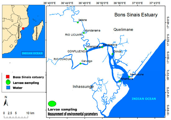
Figure 1.
The Bons Sinais Estuary (Mozambique) with defined sampling areas and points. Larvae samples were taken from Marrubune, Nhambire (lower estuary), Olinda, Chuabo Dembe, Karungo, Inhangome (middle estuary), Mundanama, and Hilalane (upper estuary).
The climate of the central part of Mozambique, where the BSE is located, is subtropical humid with a hot and wet summer from November to April and cooler and drier winters from May to October [38,39,40]; the mean annual precipitation and temperature are approximately 1400 mm and 25 °C, respectively. Using long-term records of precipitation and temperature of Quelimane City (1961–2000), ref. [40] found that the wettest period is from December to March, during which the precipitation ranges from 200 to 250 mm monthly. From May through October, precipitation is less than 100 mm; August, September, and October are the driest months, with less than 50 mm of precipitation. April and November are transitional between the wet and dry seasons, with average rainfalls of approximately 150 mm and 75 mm, respectively [40]. Monthly mean flow data for the main rivers in central Mozambique indicate that most of the runoff occurs during the flood period from January to April. The estuary receives an average of 500–840 m3 s−1 of freshwater per year from the Cuacua and Licuar tributaries [40]; the estuary is classified as a meso- to macro-tidal system with a tidal range of 4 m during spring tides [40].
2.2. Larvae Sampling
Fish larvae were collected using horizontally towed plankton nets (0.40 m in diameter and 1.5 m in length with 500 μm mesh sizes) at 8 selected sampling stations (Figure 1). In the lower estuary, sampling was conducted at two stations; at four stations in the middle estuary (two before the confluence of the tributaries and two after); and two in the upper estuary. The net used to sample the subsurface waters (at a depth of approximately 0.5 m for 05 min) was towed by a boat at a constant velocity, near the estuary margins. For each tow, a flowmeter (Hydro-Bios, manufactured by Hydro-Bios Apparatebau GmbH and sourced from Am Jägersberg 5-7, 24161 Altenholz, Germany) was attached to the net to measure the flow. The initial and final values of the flowmeter were recorded in order to calculate the volume of the filtered water.
Samples were collected monthly during daylight hours, during spring tides, from January 2018 to June 2021. Collections were carried out on two successive days to sample under approximate tidal ranges [41]. During plankton tows, water environmental parameters, including temperature and salinity, were measured by a metered YSI multi-parameter probe, and water transparency was measured using a Secchi disc.
After each tow, the zooplankton samples were transferred from the bucket of the net to containers and immediately fixed in 4% buffered formalin (pH = 8) to avoid shrinkage, mainly in newly hatched, yolk-sac larvae [42]. In the laboratory, a stereomicroscope was used to sort the fish larvae from other zooplankton before preservation in 99% analytical alcohol [43]. The density of larvae in each trawl was expressed as N°/100 m3, where the volume of water (m3) filtered by the net was determined from the flowmeter reading [41,44]. The identification of fish larvae of the ichthyoplankton samples was based on their shape, pigmentary and morphometric features, and in more advanced stages, on their meristic characteristics [42,45,46,47,48].
2.3. Data Analysis
Species richness and species diversity were estimated by estuarine zone. Species richness refers to the number of species, and species diversity to the Shannon–Wiener (H’) index [49]. Descriptive statistics were used to analyze the relative abundance of the larval taxa and larval growth stages (pre-flexion, flexion, and post-flexion). Analysis of variance (ANOVA) was used to evaluate the differences in larval diversity across estuarine zones, larval densities among estuarine zones (comprising eight locations), and months. Three estuarine zones were delineated: lower, middle, and upper. A t-test was used to compare larval density between seasons.
According to the local climate pattern, the wet season includes the period from November to April, whereas the dry season is from May to October. The spatial variation in the environmental parameters was determined using ANOVA, whereas a t-test was used to analyze seasonal changes after log(x + 1) data transformation. Correlation was used to analyze the relationship between the larval density and environmental parameters (salinity, temperature, and water transparency) after log(x + 1) data transformation.
The spatiotemporal variation in the structure of the fish larval assemblages was evaluated using permutational multivariate analysis of variance (PERMANOVA), constructed with the log(x + 1)-transformed abundance and Bray–Curtis similarity matrix, and testing with 9999 residual permutations under a type III (partial) model [50]. In addition, the spatial variation in the larval assemblage and the relationship between larval abundance and the environmental parameters were examined using canonical correspondence analysis (CCA) [51]. A complementary DistLM (distance-based linear model) was also performed to select the best explanatory environmental parameters. DistLM was used for the ichthyoplankton abundance log(x + 1)-transformation and Bray–Curtis similarity matrix, while data normalization and the Euclidean distance matrix were applied to environmental parameters [52]. Statistical analyses of the frequency of occurrence, larval density by zone, relative monthly abundance, canonical analysis, percentages of larvae in each larval stage by taxa, and length classes mainly included the most abundant taxa.
3. Results
3.1. Environmental Parameters
There was a significant variation in temperature on a seasonal basis (p < 0.05) with higher values in the wet season and lower values in the dry season in the three estuarine zones (Table 1). Within seasons, no significant changes in temperature were observed among estuarine zones (p > 0.05); therefore, the observed average values were, to some extent, conservative. Monthly variations in temperature among estuarine zones also had a conservative pattern. In the three zones, higher average temperatures were recorded from November to March (29 to 31.5 °C), whereas the lowest values were observed during June and July (23.5 and 26.6 °C).

Table 1.
Variations in temperature, salinity, and transparency by month and estuarine zone. The numbers represent averages and the standard error. The superscripts on the months refer to the seasons: W for wet and D for dry. The same superscript letter “a,a; b,b” on the environmental parameter averages indicate the absence of a significant difference within a season, whereas different letters “a,b; b,c” indicate significant differences.
Significant variations in salinity were observed among estuarine zones, as well as between seasons. Within seasons, salinity decreased toward the upper zone in both the dry and wet seasons. However, in the dry season, no significant variation in salinity was found between the middle and lower zones. Within estuarine zones, significant differences in salinity were found between dry and wet seasons in the middle and upper zones, but not in the lower zone. In the lower estuary, the highest average values were recorded from June to December when salinity exceeded 25, whereas the lowest average was recorded in March (15.5 ± 9.9). In the middle zone, the highest average values occurred from September to November (not in sequential order, 28.7 ± 0.6 to 30.5 ± 0.9), whereas the lowest occurred in March (5.3 ± 7.4). In the upper estuary, salinity conditions typical of fresh water were recorded from January to July and in December when the average salinity was less than 5. The lowest average was recorded in January and March (0.1 ± 0), whereas the highest was recorded in October (25.5 ± 3.5). The monthly average values showed that a major salinity gradient among estuarine zones occurred at the peak of the wet season (December to March) and in early dry season (May to July).
Water transparency was higher in the lower estuary than in the middle and upper estuaries in both the dry and wet seasons (p < 0.05); however, no significant variation was found between the upper and middle estuary (p > 0.05). Within estuarine zones, a significant difference was found between the dry and wet seasons in the upper zone (p > 0.05) but not in the lower and middle zones (p > 0.05). The average seasonal water transparency values in the middle and upper zones were higher in the wet than in the dry season. Despite the fact that no significant differences were found in the middle zone between seasons, a period of relatively low water transparency was observed from March to May (ranging from 16.5 ± 7.4 to 24 ± 7.9 cm).
3.2. Larval Taxa Composition, Abundance, Distribution, and Development Stage
A total of 22 fish larval taxa were identified among families, genera, and species. In terms of richness (number of taxa) variation by zone, 11 taxa were identified in the lower, 21 in the middle, and 13 in the upper zone. The middle zone had the highest Shannon–Wiener index (0.68 ± 0.07), followed by the upper zone (0.38 ± 0.07) and the lower zone (0.34 ± 0.08), with p < 0.01. Eight taxa dominated larval abundance, accounting for 97.2% of the total abundance. It was not possible to identify some taxa at the species level due to the delicate morphology of the fish larvae, the somewhat challenging sampling procedures, and the absence of specific literature. Some larval taxa were identified at the family level, namely, Gobiidae, Clupeidae, Leiognathidae, Blennidae, Polynimidae, Mullidae, Ariidae, Tetraodontidae, Sparidae, Ophichthidae, Mugilidae, Lutjanidae, Cynoglossidae, Cichlidae, and Gerreidae Gobiidae (54%), while Ambassis sp. (19.2%) and Thryssa sp. (9.7%) were the three most abundant taxa (Figure 2). The relative abundance of 14 taxa was less than 1% (Figure 2). Species of socio-economic importance accounted for 23.1% of the total relative abundance, namely, Thryssa sp. (9.7%), Clupeidae (6.2%), S. sihama (2.9%), J. dussumieri (2.5%), P. ditchela (1%), P. kaakan (0.6%), Cichlidae (<0.1%), and Mugilidae (<0.1%).
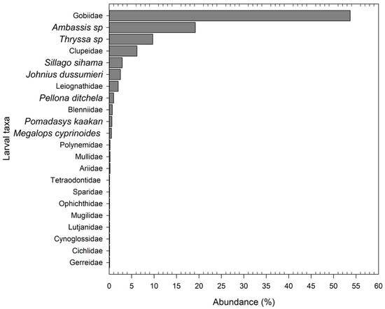
Figure 2.
Relative abundance of fish larvae in the Bons Sinais Estuary.
A significant variation in larval density (N°/100 m3) was observed among months, seasons, and estuarine zones. The highest densities were found at the sampling locations of the middle estuary zone. Therefore, the aggregated density averages by zones showed that the middle zone had a higher value than the lower and upper zones (Table 2). Furthermore, a significant difference was also found between the dry and wet seasons, with higher density in the wet season.
Table 2.
Larval abundance and density by sampling location, estuarine zone, and season. ANOVA was used to compare larval densities among sampling locations and among estuarine zones. Student’s t-test was used to compare densities between seasons.
Monthly average densities showed that lower values were recorded from April to August, with a minimum in June (10/100 m3), whereas high values were observed from September to March, with a peak in November (Figure 3).
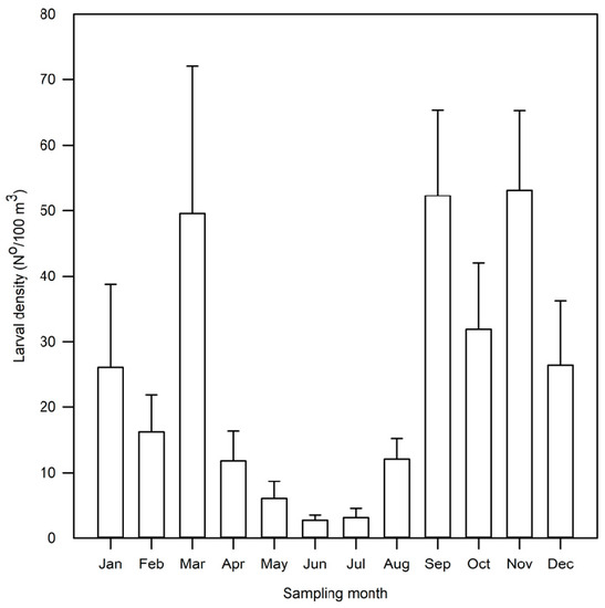
Figure 3.
Variation in larval density by month (p < 0.001). Bars indicate the monthly average (N°/100 m3) and standard deviation.
There were no significant differences in the larval density among estuarine zones for most of the larval taxa, although the averages differed in absolute values (Table 3). However, a significant difference was found in Gobiidae, the highest average density of which was found in the lower estuary. The frequency of occurrence (percentage of samples in which the taxa were identified) was lower than 50% for all taxa sampled in this study. Ambassis sp. and Gobiidae are the few taxa that had a frequency of occurrence higher than 10%. Gobiidae had concurrently the highest average density and frequency of occurrence. Larvae of Ambassis sp., Clupeidae, Thryssa sp., Gobiidae, J. dussumieri, Leiognathidae, and S. sihama were widely distributed in the estuary despite the distinct densities in the three estuarine zones.
Table 3.
Larval density and frequency of occurrence in relation to estuarine zones. The frequency of occurrence refers to the percentage of samples in which the larval taxa were sampled.
The monthly distribution of larval abundance varied by taxa. For most larval taxa, the lowest abundance was recorded in June and July, whereas the highest occurred in the period from September to March. More fish larvae were identified in the period from September to December, whereas fewer taxa were identified from January to August (Table 4). Gobiidae and Ambassis sp. larvae were identified in all months but with marked monthly variations. However, P. ditchela and P. kaakan larvae were sampled in a restricted period from September to December.
Table 4.
Monthly occurrence and relative abundance (%) of the most abundant larval taxa in the Bons Sinais Estuary.
Most of the sampled larvae were in the post-flexion stage (62.05%), whereas the flexion stage accounted for 7.22%, and the pre-flexion stage accounted for 30.72%. Larvae in the post-flexion stage were present in all larval taxa with the exception of Mullidae; the post-flexion stage was most predominant in Blennidae (76.92%), Thryssa sp. (92.02%), Clupeidae (68.91%), and S. sihama (46.43%). For J. dussumieri, the most abundant larvae stage was flexion, which accounted for 56.25% (Figure 4). The pre-flexion stage was most predominant in Gobiidae (53.42%), followed by S. sihama (41.07%) and J. dussumieri (20.83%). Only three larval taxa had the three larval developmental stages, namely, J. dussumieri, S. sihama, and Gobiidae.
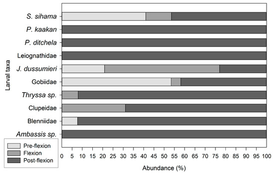
Figure 4.
The proportion of larvae among the most abundant taxa in each development stage.
In the middle and upper zones, there was a predominance of larvae in the post-flexion stage, 69% and 86.9%, respectively, whereas in the lower estuary, most larvae were in the pre-flexion stage (74.94%). The proportion of larvae in the pre-flexion stage decreased from the lower estuary to the upper estuary, whereas for the flexion and post-flexion stages, the proportions decreased in the opposite direction. Therefore, the middle estuary had intermediate proportions of larvae in the three stages of development (Figure 5).
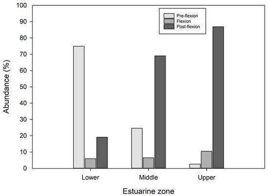
Figure 5.
The proportion of fish larvae by developmental stage within the estuarine zones.
In Gobiidae and S. sihama, the pre-flexion specimens dominated the lower zone (Figure 6).
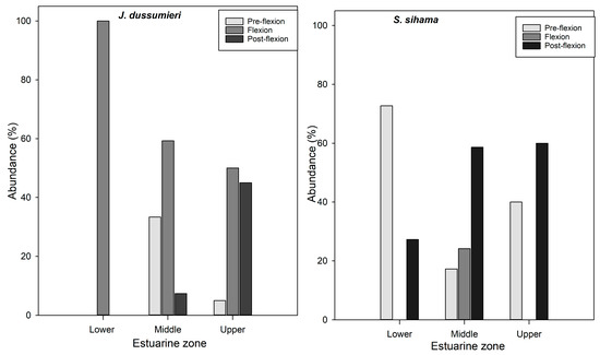
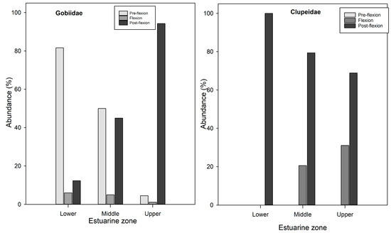
Figure 6.
Distribution of fish larvae in different developmental stages across estuarine zones in the Bons Sinais Estuary. The figure shows the larval taxa with fairly high abundances in the three developmental stages.
In some taxa, the distribution of length classes was wide, consisting of specimens of a few millimeters and relatively larger ones, such as Gobiidae, S. sihama, J. dussumieri, and Ambassis sp. Other taxa had a very narrow length class distribution, such as P. ditchela and Leiognathidae (Figure 7 and Table 5). These results are related to the presence and abundance of larvae in each taxon in the pre-flexion, flexion, and post-flexion stages.
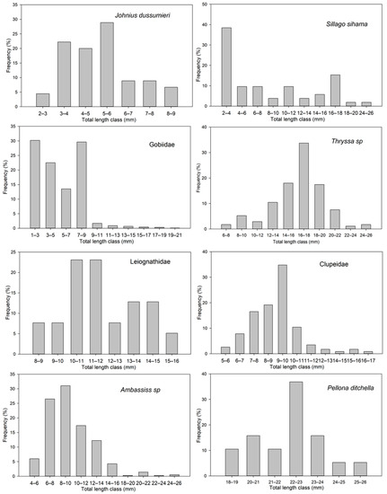
Figure 7.
Total length classes (mm) of the eight most abundant fish larval taxa in the Bons Sinais Estuary.
Table 5.
Total length range and the average of the developmental stages for the most abundant larval taxa.
3.3. Relationship between Environmental Variables and Larval Assemblage
A significant positive correlation between larval density (N°/100 m3) and temperature (p < 0.01) and a significant negative correlation between density and transparency (p = 0.01) were found (Figure 8). However, no significant correlation was found between larval density and salinity (p = 0.178). High larval densities (e.g., higher than 50/100 m3) were mostly associated with a temperature range from 26 to 32 °C and a water transparency range from 20 to 40 cm. In relation to the salinity gradient, the highest larval densities were found mostly for high values (25 to 33). However, there were peaks of larval density that were associated with lower values of salinity (0 to 5). Therefore, the scatter plot shows peaks of larval densities at the lower and upper limits of the salinity range (Figure 8).
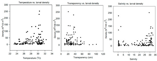
Figure 8.
Scatter plot of larval density (N°/100 m3) and environmental parameters (temperature, water transparency, and salinity).
The two-way PERMANOVA results showed that there were no significant interactions between the estuarine zone and the season in both comparisons of larvae abundance and density (season × estuarine zone: p > 0.05). Conversely, the larvae density and abundance among the estuarine zones and between seasons showed significant differences (p < 0.05) (Table 6).
Table 6.
Results of the two-way PERMANOVA (9999) comparing the assemblage structure of fish larvae using abundance and density data according to the factors: estuarine zone and season. df = degrees of freedom; MS = mean square; F = F statistics.
The first canonical axes of the CCA explained 66.02% of the variance in the taxa–environment parameter relationships, whereas the second axis explained 33.98% (Figure 9 and Table 7). For some larval taxa, there was a clear relationship between their assemblages and environmental parameters. For instance, Blennidae, J. dussumieri, S. sihama, and Gobiidae may be linked to intermediate levels of salinity and transparency.
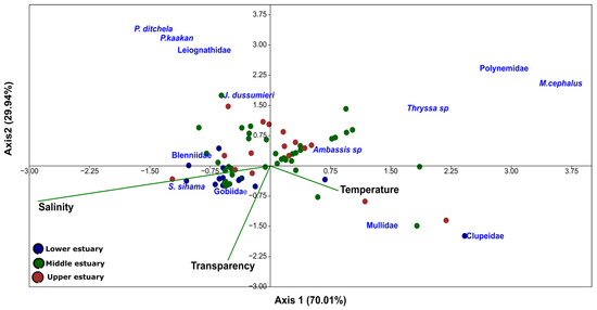
Figure 9.
Canonical correspondence analysis of fish larval distribution in the Bons Sinais Estuary. The CCA was performed using the most abundant larval taxa of the Bons Sinais Estuary. Arrows represent quantitative environmental variables, and the nominal variable (estuarine zone) is indicated by symbols. The angle between two vectors reflects the degree of correlation between variables. The angle between a vector and each axis is related to its correlation with the axis.
Table 7.
Results from the canonical correspondence analysis (CCA) of fish larval taxa in the Bons Sinais Estuary.
According to the environmental parameter vectors of CCA and the results of the complementary distance-based linear model DistLM (Table 8), the combination of water transparency, salinity, and temperature gradients adequately explained the variation in the fish larval assemblage. Furthermore, the DistLM results showed that the variation in the fish larval assemblage related to each environmental parameter or the paired selections had small differences.
Table 8.
Distance-based linear model (DistLM) of Bray–Curtis similarities between samples in terms of the abundance of fish larvae relative to the environmental parameters. RSS = residual sum of squares; R-squared = the absolute amount of variation as a proportion of the total variation.
4. Discussion
The results of this study showed a clear representation of the post-flexion phases of most sampled taxa in the BSE, especially in the middle and upper areas. This can be explained by the environmental and biological characteristics of the system. A significant presence of early phases in the lower estuary was also recorded, showing the relevance of the coastal area for the spawning of some of the fish species studied.
4.1. Environmental Parameters
The environmental parameters varied according to the climate regime of the area where the BSE is located. While there was significant seasonal and spatial variation in salinity and water transparency, the temperature variation was significant at the seasonal level but conservative across the estuary zones.
Salinity changes in estuaries reflect the degree of marine water dilution due to the inflow of freshwater from the continental watershed and precipitation [53]. The lowest values of salinity in the three estuarine zones occurred in the wettest months and the highest in the driest period. Considering that the wet season begins in November [38], the decrease in salinity in the estuary was evident from December, when the flows of the rivers that supply water to the estuary achieved significant increases. On the other hand, in the upper estuary, salinity averages of less than 5 were still recorded in the first months of the dry season, namely, May to June. A previous study found similar results [54] in the BSE by noting strong spatial gradients and seasonal variations in salinity, and concluded that the estuary is river-dominated during the wet season and sea-tide-dominated during the dry season.
Regarding temperature in some tropical and temperate estuaries, this parameter has lower spatial gradients [55,56,57]. However, it changes more with seasonality [55,56,58,59], as was found in this study; stronger variations were observed with the change in season. Estuarine water temperatures tend to reflect riverine conditions during increased runoff in the wet season, with the sea having a stronger influence during dry conditions [60]. Spatial and seasonal gradients have been observed in some temperate estuaries [61,62]. The spatial gradients can result from the differential heating and cooling between the upper and lower estuary, and the effect of tides [62].
The optical properties in the BSE’s middle and upper zones had similar patterns, as there were no significant differences in water transparency between the zones; however, the average values of both zones were lower than that of the lower estuary. In estuaries, the spatial gradient in water transparency is linked to the concentrations of dissolved and particulate organic matter (which typically increase from lower to upper estuarine reaches) and cohesive sediments in the water column [63]. Therefore, low values of water transparency occur toward lower salinity waters, as found in this study. In terms of seasonality, the lowest water transparency usually occurs in the wet season due to increased organic matter input from the watershed [64]. However, the location of the zone of maximum turbidity (estuarine turbidity maximum—ETM), which corresponds to the lowest water transparency, varies according to the location of the freshwater–saltwater interface, which in turn strongly depends on the river flow and the tidal flow [64,65]. In this way, the position of the ETM changes seasonally [66,67], moving downstream during the wet season, but during the dry season or obstructed river flow, it moves to the upper estuary [31,65,68,69]. Measurements in the upper zone were likely taken in locations that, in the dry season, were at the interface between freshwater and seawater, with the lowest water transparency, but the interface moved downstream in the wet season. On the other hand, erosion and the accumulation of sediments seaward are features of estuaries in which ebb currents are stronger than flood currents [70]—as in the BSE—where ebb currents peak in the wet season [54].
4.2. Larval Taxa Composition, Abundance, Distribution, and Development Stage
In this study, few taxa dominated the abundance of fish larvae; thus, the Gobiidae, a group mostly formed by estuarine resident species, alone accounted for 54% of the ichthyoplankton. Species of socio-economic importance accounted for approximately 23% of the total relative abundance, with major proportions of Thryssa sp. and Clupeidae, probably Hilsa kelee and Sardinella albella, due to their representation in adult fisheries [71]. Larval density and abundance differed greatly among the estuarine zones, seasons, and months.
Although larvae and juvenile fish density tend to be higher in estuaries than in adjacent habitats, species diversity associated with their nursery areas is lower than that in the adjacent marine areas [72]. High species diversity in juvenile and adult fish, but a contrastingly low species diversity in ichthyoplankton, has been found in many estuaries, for example, the Matang Estuary, Malaysia [73], and the St. Lucia Estuary, South Africa [20,22]. The significant fluctuation in salinity in estuaries is a key factor for the reduction in estuarine ichthyoplankton diversity and the dominance of a few estuarine resident or spawning and marine euryhaline species [73]. Other factors that influence the diversity and abundance of fish larvae and juveniles include the geomorphology of the estuary, habitat heterogeneity, and a well-established environmental gradient. It has been widely recognized that larger estuaries with high freshwater discharge volumes, long transition areas, and well-developed spatial salinity gradients host more species and tend to have good recruitment of estuarine-dependent species during their early life stages [23,74,75,76]. In Bons Sinais, increased freshwater discharge and a well-developed salinity gradient occurred at the peaks of the wet season and in the early dry season.
The community composition and relative abundance of different taxa sampled in this study have similarities to those reported for Indo-Pacific estuaries [33,73,77,78], where Gobiidae is widespread and is usually the most abundant larvae in coastal zooplankton samples [42,79]. Gobiidae larval dominance, which has been likewise observed in many estuaries worldwide [30,43,80], may be related to the fact that it represents the highest number of fish species [42], with a relatively long duration of their larval phase [81], and the fact that the species undertake estuarine spawning as well as residency [6,33]. In addition, the benthic reproductive strategy in the family avoids the transportation of eggs out of the estuary, making them less subject to environmental fluctuations in surface waters [82]. The predominance of larvae hatching from benthic eggs rather than species that spawn pelagic eggs is also a common feature of nearshore/inshore waters [83], as seen in our study with the Gobiidae dominance. The relative abundance of Ambassis sp. found in this study was by far greater than that in other estuaries of the Indo-Pacific region [34,78,84]. However, a significant occurrence of the same genera of larval specimens was found in Pattani Bay [85]. In the St. Lucia estuarine system, A. productus, A. natalensis, and A. gymnocephalus represent more than 12% of the adult fish population [86].
Engraulidae (represented here by Thryssa sp.) and Clupeidae were among the most abundant taxa in the BSE. Similar results have been found in many temperate and tropical estuaries [34,87,88,89]. The high abundance of larvae of both families in the BSE may be related to their tolerance to salinity fluctuations and the high productivity of the area, as the spawning in these taxa mostly takes place inshore, but post-larval stages utilize the estuary and adjacent coastal waters as nursery grounds [73]. The Clupeidae H. kelee and S. albella and the Engraulidae T. vitrirostris and T. setirostris were the expected species in our samples because these taxa account for a significant proportion of the bycatch of a semi-industrial fishery along the Mozambique coast and represent the main component of the multispecies artisanal fishery inshore and in estuaries [71,90].
In general, the relative abundance of larvae of less than 5% is similar to that found in other Eastern African estuaries. However, for S. sihama, the estuary has a relatively higher percentage than that in the Mngazi Estuary [13] and other subtropical South African estuaries [75]. Conversely, the relative abundances of Mugilidae and Sparidae in Bons Sinais are lower in comparison to the data obtained in some South African estuaries [23,75,78]. These differences may be related to the tolerance of these taxa in relation to the salinity variation pattern in the estuary. S. sihama has significant tolerance to low salinity levels of 3 [91], including larvae and early juveniles [92]. Most species of Mugilidae that are diadromous fish were also scarcely represented in the BSE during post-larval phases. Nevertheless, the juveniles of this family use the estuary as a migratory route to the freshwater section and return to the sea to complete maturation and spawning [93,94,95]. In the BSE, an analysis of the total length classes of the striped mullet (Mugil cephalus) revealed that mostly juveniles [96] represent the species. The lower abundance of mugilids in this study might be linked to the migration pattern of the early life stages to the estuary. For most of species of the family, the early larval phase occurs in the open sea. Then, the post-flexion specimens or early juveniles move inshore, where they spend a month before migration to the estuary in schools [97], which generally occurs at a total length of 15 to 25 mm [95,97]. However, larger juveniles of M. cephalus are usually concentrated within the littoral zone [97] and have great swimming ability, with a swimming speed of 47 cm s−1 [98] that will enable them to escape from piscivores.
Migration patterns and degree of dependence on the estuary can also explain the scarce abundance of Sparidae larvae in Bons Sinais Estuary despite adult fish of two species in the family (Crenidens crenidens and Acanthopagrus berda) being highly represented in the Zambezi Estuary [38], which flows into the same coastal area (the Sofala Bank), similar to the BSE. In Acanthopagrus berda, spawning occurs at the estuarine mouth, but the egg and early larval development take place at sea; the ingress into the estuaries is mainly during the juvenile and adult phases [99,100]. Crenidens Crenidens is regarded as a marine straggler species and the early life stages do not use the estuaries as growth grounds [95].
Despite the extremely low percentage (lower than 1%) of Cichlidae larvae, the occurrence of adults and juveniles in the BSE has been confirmed, mostly Oreochromis mossambicus [96]. In general, the occurrence of adults and larvae of O. mossambicus is confined to the upper reaches in permanently open estuaries due to physiological restrictions that pertain to limited high-salinity tolerances [101,102], as well as increased competition for food and higher predation rates by piscivorous fishes and birds [102]. In addition, the species prefer shallower areas and avoid higher water velocities; for additional shelter from predators, the juveniles utilize vegetated littoral zones until they reach maturity [101], but these areas were not included in our sampling procedures. The reproductive strategies in the Oreochromis genera can influence the sampling of early life phases as the females mouthbrood the eggs and larvae, and the fry are released at the swim-up stage when the swim bladder develops [103].
Most fish larvae were in the post-flexion stage; likewise, it was the most abundant larval stage for most of the identified taxa. In terms of zonation, there was a predominance of the pre-flexion stage in the lower estuary and of the post-flexion stage in the middle and upper zones. Typically, most larvae of marine species ingress into estuaries as post-flexion larvae and early juveniles [84] with abilities for active swimming and the selection of favorable margin current regimes for movement within the estuary [29,104].
Gobiidae was the only family with the most abundant larvae in the pre-flexion stage. In estuaries, the Gobiidae family is represented mainly by resident species that spawn within the estuaries [95]. Ambassis sp. also belongs to the estuarine taxa; the absence of pre-flexion and flexion larvae in the genus despite the wide distribution along the estuarine zones may be explained by the short duration of the pre-flexion stage [42]. On the other hand, some species in the genus spawn inshore [105] due to a limited tolerance to low-salinity habitats. A substantial percentage of pre-flexion larvae in S. sihama and J. dussumieri, regarded as marine species [106], may be an indication that the spawning of some populations occurs at the mouth of the estuary or near the coast.
The average total length of Clupeidae, Gobiidae, Thryssa sp, J. dussumieri, and S. sihama at the notochord flexion stage is within the range found in the bibliography for Indo-Pacific fish larvae [42], which refers to the families to which the taxa belong. Therefore, this study determined the average total length at the notochord flexion stage at the species level in S. sihama and J. dussumieri, whereas for Thryssa sp., it was at the genus level. Specimens longer than 5 mm dominated the total length classes in the most abundant marine larval taxa; that is, the minimum size that the larvae need to produce speeds great enough to influence dispersal, after notochord flexion, and the concomitant formation of the caudal fin [107].
The dispersion and survival of larvae greatly depend on their swimming performance, which allows them to overcome strong currents and ingress, be retained in estuaries, and search for optimal habitats for feeding and protection from predators. According to the critical swimming speed (CSS) of some larval fish families, currents in estuaries are somewhat stronger and stifle the ingress and retention of larvae. For instance, the CSS of 18.7 cm/s for Clupeidae [108], CSS of 18.4 cm/s for Blennidae [108], and CSS of 22.1 cm/s Scianidae [109] are lower than the maximum currents in the estuary of around 100 cm/s determined by [54] at spring tides. Under such severe hydrodynamic conditions, some species may use different strategies to be retained in the estuary, including short-range directional horizontal swimming against the axial currents, vertical migration, and the use of residual upstream flows, especially over shallower areas [29].
There was a consistent match among the relative abundances, densities, and frequencies of occurrence of the taxonomic groups. However, Clupeidae and Thryssa sp. had a low frequency of occurrence in the samples despite high relative abundances and high densities. This may be related to the seasonality of spawning, but as they are schooling taxa [42], fewer samplings can catch a considerable number of larvae.
An evident spatial variation in the overall larval density and taxa group diversity was found, as the middle zone differed greatly from the lower and upper zones. Furthermore, except for the Tetraondotidae, all taxa groups were sampled in the middle zone, suggesting that it has suitable conditions for many ichthyoplankton taxa; the upper and lower zones were shown to lack some taxa. Typically, peak larval density is associated with the transitional middle zone where environmental parameters (salinity, temperature, and water transparency) have intermediate values, generally high levels of food availability, as well as reduced competition [10,29,75]. However, the larval density of different taxa displayed different patterns in relation to the estuarine zones, despite significant differences being observed only in Gobiidae. The assemblage of juvenile fish in coastal nursery areas is mainly dependent on the individual species’ tolerance to the salinity gradient, with some taxa located mainly in estuarine waters and others more abundant in marine areas [102,110].
The overall larval density was higher in the wet season, and in terms of monthly variation, higher densities were observed from the late dry season (September, October) to the peak of the wet season (March), whereas lower densities were found in the early dry season (May to August). Therefore, there is a link between larval density variation and the precipitation cycle, which in turn affects the river flow and salinity gradients. The increase in river flow in the wet season is associated with increased organic detritus availability that supports the ecosystem’s food web and is the cue for fish ingress. In addition, the wet season is associated with higher temperatures that promote larval growth and lower water transparency, an essential factor for the protection of larvae against predation [35,111]. Increased river flow intensifies the size of estuarine plumes, which can reach the bottom by vertical mixing induced by strong spring tides [112]. The gradients in environmental parameters, namely, salinity, temperature, and turbidity, between the plume water and the saltier seawater are important factors for fish larval migration. Larvae use sense acuity and behavioral response to swim along the increasing cue concentration to ingress into the estuary [24]. There is a reduction in river flow from the early dry season (May to August) and a lowering of water temperature, which can explain the lower larval density found in this period. In the BSE, the current velocities are higher in the dry season (up to 100 m/s at spring tides) compared to the wet season, which are around 60 cm/s for the spring tides [54], a condition that may favor a major ingress of larvae in the later season.
A relative abundance distribution of different larval taxa among different months followed the same seasonality pattern displayed by the density, as the highest relative abundances were recorded from the late dry season (September) to the peak of the rainy season. From the distribution of the relative abundance among different months, it can be argued that spawning in Gobiidae and Ambassidae is continuous throughout the year, whereas Blennidae, Pellona ditchela, and Pomadasys kaakan have more restricted spawning periods.
4.3. Relationship between Environmental Variables and Ichthyoplankton Assemblages
In this study, correlation and multivariate analyses revealed a strong relationship between larval density and environmental parameters. In fact, salinity, temperature, and turbidity are considered crucial abiotic factors influencing the ichthyoplankton assemblage in a particular habitat [10].
The positive correlation between larval density and the temperature validates the fact that high densities were recorded in a period of relatively high temperatures of the year, in the late dry season and during the wet season. Similar to this study, a positive correlation between larval density and temperature was found in many other studies worldwide [35,73,113]. A strong correlation was found between water transparency and larval density. Reduced water transparency conditions provide greater protection to larvae from predation by preventing predators from seeing the larvae [6,114], but especially due to the cues provided by turbidity in high freshwater pulses in the wet season [24].
Despite the consensus according to which estuary larval density is strongly related to temperature, salinity, and turbidity [115], not all studies verify a positive correlation for the three parameters. For instance, studies undertaken in different estuarine systems [35,75,116] did not find positive correlations between larval density and salinity. In addition, in the present study, the weak correlation between larval density and salinity may result from the fact that there were density peaks in some larval taxa for both lower and high salinities. In fact, the highest relative abundances of Clupeids and Thryssa sp. occurred in January and March, respectively, when salinity was lower. The highest relative abundance of Ambassis sp., Gobiidae, Leiognathidae, and P. ditchela occurred from September to November, when salinity was high.
Multivariate analyses (PERMANOVA, distance-based linear model, and canonical analysis) confirmed significant spatial–temporal variation in larval abundance and its strong relationship with environmental parameters (temperature, salinity, and transparency). The distance-based linear model showed that salinity, temperature, and water transparency had a strong influence on larval abundance and density. The CCA elucidated the pattern of variation in larvae abundance at the taxa level in relation to the environmental parameters, revealing that each taxon had particular optimal levels of environmental factors. Higher larval abundance was associated with intermediate conditions of salinity and lower water transparency.
5. Conclusions
The results show that Gobiidae dominated the Bons Sinais Estuary ichthyoplankton assemblages, being present along the whole estuary and in every sampling month.
Most of the sampled fish larvae were in the post-flexion stage. Larvae in the pre-flexion stage dominated the lower estuary, whereas the post-flexion stage dominated the middle and upper zones. At the community level, salinity, water transparency, and temperature had a strong influence on larval abundance.
Larval density was higher from the late dry season (September, October) to the peak of the wet season (March); among estuarine zones, the highest density was in the middle zone. The results show that in most estuary-associated fish species the spawning is seasonal and synced with the increased temperature, decreased salinity, and increased turbidity of the wet season. This enables larval and early juvenile occupation of the estuary when river flow and plankton productivity increase.
This study demonstrated that the Bons Sinais Estuary serves as a nursery ground for some fish species with socio-economic value for larval growth, namely, Thryssa sp., Clupeidae, S. sihama, J. dussumieri, P. ditchela, P. kaakan, and Mugilidae. These results have implications for the local ecosystem management strategies that need to be improved and consider the estuary as a critical habitat for marine species, juveniles’ growth, and the subsequent recruitment of the open-sea populations.
The fact that post-flexion larvae, which are less vulnerable to capture by standard plankton nets, dominated the marine taxa, has implications for larval catchability and therefore sampling results. There is a need to use complementary sampling gears to increase the catchability of larvae with different movement behaviors. To increase the catchability of larvae with different diel behavior it is necessary to consider sampling in both daylight and at night.
Author Contributions
Conceptualization, J.M. and M.A.T.; methodology, J.M. and M.A.T.; software J.M. and F.L.; validation, F.L. and M.A.T.; formal analysis, F.L.; investigation, J.M.; resources, J.M. and M.A.T.; data curation, F.L.; writing—original draft preparation J.M.; writing—review and editing, J.M. and M.A.T.; visualization, J.M.; supervision, M.A.T. and F.L.; project administration, F.L. and J.M.; funding acquisition, J.M., M.A.T. and F.L. All authors have read and agreed to the published version of the manuscript.
Funding
This work was funded by Project BIOFISH-QoL (Reference Proposal: 330785505/2018): An integrative approach for enhancing the quality of life in fishing communities of the “Bons Sinais” Estuary (Mozambique) funded by Fundação para a Ciência e a Tecnologia (FCT I.P.) and Aga Khan Development Network (AKDN). The Ph.D. fellowship awarded to J. Mocuba was funded by the Mozambican Ministry of Science and Technology, Higher and Technical–Professional Education, and supported by the Western Indian Ocean Marine Science Association (WIOMSA) within the Marine Research Grant (MARG) program. F. Leitão has received Portuguese national funds from FCT under the contract program DL57/2016/CP1361/CT0008 and FCT 2022.04803.CEECIND. This study received Portuguese national support from FCT—Foundation for Science and Technology through projects UIDP/04326/2020 and LA/P/0101/2020.
Data Availability Statement
The data presented in this study are available upon request from the corresponding author. The data are not publicly available since the research project is still ongoing.
Acknowledgments
The authors would like to thank the National Institute for Fish Inspection of Mozambique (INIP) for the initial provision of laboratory equipment, and the former undergraduate students M. Nhaca, C. Mausse, and A. Piedade from the Eduardo Mondlane University for their collaboration in field and laboratory activities. Special thanks are extended to the colleagues Sara Tembe, Noca Furaca, Inocência Paulo, and Bonifácio Manuessa for coordinating the logistics for the fieldwork as well as for participating in the sampling tasks. Joana Cruz provided valuable assistance to identify some larval taxa.
Conflicts of Interest
The authors declare that they have no known competing financial interest or personal relationships that may appear to influence the work reported in this paper.
References
- June, F.C.; Chamberlin, J.L. The role of the Estuary in the Life History and Biology of Atlantic Menhaden. 1959. Available online: http://hdl.handle.net/1834/29218 (accessed on 27 April 2023).
- McDowall, R.M. The Role of Estuaries in the Life Cycles of Fishes in New Zealand. In Proceedings New Zealand Ecological Society; New Zealand Ecological Society (Inc.): Invercargill, New Zealand, 1976; Volume 23, pp. 27–32. [Google Scholar]
- Wallace, J.H.; Kok, H.M.; Beckley, L.E.; Bennett, B.; Blaber, S.J.M.; Whitfield, A.K. South African estuaries and their importance to fishes. S. Afr. J. Sci. 1984, 80, 203–207. [Google Scholar]
- Blaber, S.J.M.; Milton, D.A. Species composition, community structure and zoogeography of fishes of mangrove estuaries in the Solomon Islands. Mar. Biol. 1990, 105, 259–267. [Google Scholar] [CrossRef]
- Whitfield, A.K. Life-history styles of fishes in South African estuaries. Environ. Biol. Fishes 1990, 28, 295–308. [Google Scholar] [CrossRef]
- Blaber, S.J.M. Tropical Estuarine Fishes: Ecology. Exploit. Conserv. 2000, 2, 148–157. [Google Scholar]
- Bhat, M.; Nayak, V.N.; Chandran, S.; Ramachandra, T.V. Fish distribution dynamics in the Aghanashini estuary of Uttara Kannada, west coast of India. Curr. Sci. 2014, 106, 1739–1744. [Google Scholar]
- Sheaves, M.; Baker, R.; Nagelkerken, I.; Connolly, R.M. True value of estuarine and coastal nurseries for fish: Incorporating complexity and dynamics. Estuaries Coasts 2015, 38, 401–414. [Google Scholar] [CrossRef]
- Moyle, P.B.; Cech, J.J. Fishes: An Introduction to Ichthyology; Prentice Hall: Upper Saddle River, NJ, USA, 2000; 612p. [Google Scholar]
- Whitfield, A.K.; Pattrick, P. Habitat type and nursery function for coastal marine fish species, with emphasis on the Eastern Cape region, South Africa. Estuar. Coast. Shelf Sci. 2015, 160, 49–59. [Google Scholar] [CrossRef]
- Nagelkerken, I.; Sheaves, M.; Baker, R.; Connolly, R. The seascape nursery: A novel spatial approach to identify and manage nurseries for coastal marine fauna. Fish Fish. 2014, 16, 362–371. [Google Scholar] [CrossRef]
- Dolbeth, M.; Martinho, F.; Viegas, I.; Cabral, H.; Pardal, M.A. Estuarine production of resident and nursery fish species: Conditioning by drought events? Estuar. Coast. Shelf Sci. 2008, 78, 51–60. [Google Scholar] [CrossRef]
- Pattrick, P.; Strydom, N.A.; Wooldridge, T.H. Composition, abundance, distribution and seasonality of larval fishes in the Mngazi Estuary, South Africa. Afr. J. Aquat. Sci. 2007, 32, 113–123. [Google Scholar] [CrossRef]
- Vasconcelos, R.P.; Reis-Santos, P.; Costa, M.J.; Cabral, H.N. Connectivity between estuaries and marine environment: Integrating metrics to assess estuarine nursery function. Ecol. Indic. 2011, 11, 1123–1133. [Google Scholar] [CrossRef]
- Dolbeth, M.; Martinho, F.; Leitão, R.; Cabral, H.; Pardal, M.A. Strategies of Pomatoschistus minutus and Pomatoschistus microps to cope with environmental instability. Estuar. Coast. Shelf Sci. 2007, 74, 263–273. [Google Scholar] [CrossRef]
- Potter, I.C.; Hyndes, G.A. Characteristics of the ichthyofaunas of southwestern Australian estuaries, including comparisons with holarctic estuaries and estuaries elsewhere in temperate Australia: A review. Aust. J. Ecol. 1999, 24, 395–421. [Google Scholar] [CrossRef]
- Houde, E.D.; Rutherford, E.S. Recent trends in estuarine fisheries: Predictions of fish production and yield. Estuaries Coasts 1993, 16, 161–176. [Google Scholar] [CrossRef]
- Able, K.W. A re-examination of fish estuarine dependence: Evidence for connectivity between estuarine and ocean habitats. Estuar. Coast. Shelf Sci. 2005, 64, 5–17. [Google Scholar] [CrossRef]
- James, N.C.; Cowley, P.D.; Whitfield, A.K.; Kaiser, H. Choice chamber experiments to test the attraction of postflexion Rhabdosargus holubi larvae to water of estuarine and riverine origin. Estuar. Coast. Shelf Sci. 2008, 77, 143–149. [Google Scholar] [CrossRef]
- Harris, S.A.; Cyrus, D.P.; Beckley, L.E. The larval fish assemblage in nearshore coastal waters off the St Lucia Estuary, South Africa. Estuar. Coast. Shelf Sci. 1999, 49, 789–811. [Google Scholar] [CrossRef]
- Cowen, R.K.; Sponaugle, S. Larval dispersal and marine population connectivity. Annu. Rev. Mar. Sci. 2009, 1, 443–466. [Google Scholar] [CrossRef]
- Harris, S.A.; Cyrus, D.P. Occurrence of fish larvae in the St Lucia Estuary, KwaZulu-Natal, South Africa. S. Afr. J. Mar. Sci. 1995, 16, 333–350. [Google Scholar] [CrossRef]
- Strydom, N.A.; Whitfield, A.K.; Wooldridge, T.H. The role of estuarine type in characterizing early stage fish assemblages in warm temperate estuaries, South Africa. Afr. Zool. 2003, 38, 29–43. [Google Scholar] [CrossRef]
- Teodósio, M.A.; Paris, C.B.; Wolanski, E.; Morais, P. Biophysical processes leading to the ingress of temperate fish larvae into estuarine nursery areas: A review. Estuar. Coast. Shelf Sci. 2016, 183, 187–202. [Google Scholar] [CrossRef]
- Baptista, V.; Costa, E.F.; Carere, C.; Morais, P.; Cruz, J.; Cerveira, I.; Castanho, S.; Ribeiro, L.; Pousão-Ferreira, P.; Leitão, F.; et al. Does consistent individual variability in pelagic fish larval behaviour affect recruitment in nursery habitats? Behav. Ecol. Sociobiol. 2020, 74, 67. [Google Scholar] [CrossRef]
- Sheaves, M.; Johnston, R.; Johnson, A.; Baker, R.; Connolly, R.M. Nursery function drives temporal patterns in fish assemblage structure in four tropical estuaries. Estuaries Coasts 2013, 36, 893–905. [Google Scholar] [CrossRef]
- Arevalo, E.; Cabral, H.N.; Villeneuve, B.; Possémé, C.; Lepage, M. Fish larvae dynamics in temperate estuaries: A review on processes, patterns and factors that determine recruitment. Fish Fish. 2023, 24, 466–487. [Google Scholar] [CrossRef]
- Chícharo, M.A.; Chícharo, L.; Morais, P. Inter-annual differences of ichthyofauna structure of the Guadiana estuary and adjacent coastal area (SE Portugal/SW Spain): Before and after Alqueva dam construction. Estuar. Coast. Shelf Sci. 2006, 70, 39–51. [Google Scholar] [CrossRef]
- Teodósio, M.A.; Garel, E. Linking hydrodynamics and fish larvae retention in estuarine nursery areas from an ecohydrological perspective. Ecohydrol. Hydrobiol. 2015, 15, 182–191. [Google Scholar] [CrossRef]
- Faria, A.; Morais, P.; Chícharo, M.A. Ichthyoplankton dynamics in the Guadiana estuary and adjacent coastal area, South-East Portugal. Estuar. Coast. Shelf Sci. 2006, 70, 85–97. [Google Scholar] [CrossRef]
- Morais, P.; Chícharo, M.A.; Chícharo, L. Changes in a temperate estuary during the filling of the biggest European dam. Sci. Total Environ. 2009, 407, 2245–2259. [Google Scholar] [CrossRef]
- Houde, E.D.; Able, K.W.; Strydom, N.A.; Wolanski, E.; Arula, T. Reproduction, ontogeny and recruitment. Fish Fish. Estuaries A Glob. Perspect. 2022, 1, 60–187. [Google Scholar]
- Neira, F.J.; Potter, I.C.; Bradley, J.S. Seasonal and spatial changes in the larval fish fauna within a large temperate Australian estuary. Mar. Biol. 1992, 112, 1–16. [Google Scholar] [CrossRef]
- Balakrishnan, T.; Sundaramanickam, A.; Shekhar, S.; Muthukumaravel, K.; Balasubramanian, T. Seasonal abundance and distribution of ichthyoplankton diversity in the Coleroon estuarine complex, Southeast coast of India. Biocatal. Agric. Biotechnol. 2015, 4, 784–794. [Google Scholar] [CrossRef]
- Guerreiro, M.A.; Martinho, F.; Baptista, J.; Costa, F.; Pardal, M.Â.; Primo, A.L. Function of estuaries and coastal areas as nursery grounds for marine fish early life stages. Mar. Environ. Res. 2021, 170, 105408. [Google Scholar] [CrossRef]
- Hedberg, P.; Rybak, F.F.; Gullström, M.; Jiddawi, N.S.; Winder, M. Fish larvae distribution among different habitats in coastal East Africa. J. Fish Biol. 2019, 94, 29–39. [Google Scholar] [CrossRef]
- Leal, M.C.; Pereira, T.C.; Brotas, V.; Paula, J. Vertical migration of gold-spot herring (Herklotsichthys quadrimaculatus) larvae on Sofala Bank, Mozambique. West. Indian Ocean J. Mar. Sci. 2010, 9, 175–183. [Google Scholar]
- Abrantes, K.G.; Barnett, A.; Marwick, T.R.; Bouillon, S. Importance of terrestrial subsidies for estuarine food webs in contrasting East African catchments. Ecosphere 2013, 4, 1–33. [Google Scholar] [CrossRef]
- Palalane, J.; Larson, M.; Hanson, H.; Juízo, D. Coastal erosion in Mozambique: Governing processes and remedial measures. J. Coast. Res. 2016, 32, 700–718. [Google Scholar]
- Mazzilli, S. Understanding Estuarine Hydrodynamics for Decision Making in Data Poor Coastal Environments. Ph.D. Thesis, University of Cambridge, Cambridge Coastal Research Unit, Cambridge, UK, 2015. [Google Scholar]
- Barletta-Bergan, A.; Barletta, M.; Saint-Paul, U. Structure and seasonal dynamics of larval fish in the Caeté River Estuary in North Brazil. Estuar. Coast. Shelf Sci. 2002, 54, 193–206. [Google Scholar] [CrossRef]
- Leis, J.M.; Carson-Ewart, B.M. The Larvae of Indo-Pacific Coastal Fishes: An Identification Guide to Marine Fish Larvae; Leis, J.M., Carson-Ewart, B., Eds.; Brill: Leiden, The Netherlands, 2000; Volume 2. [Google Scholar]
- Ramos, S.; Cowen, R.K.; Ré, P.; Bordalo, A.A. Temporal and spatial distributions of larval fish assemblages in the Lima estuary (Portugal). Estuar. Coast. Shelf Sci. 2006, 66, 303–314. [Google Scholar] [CrossRef]
- Sampey, A.; Meekan, M.G.; Carleton, J.H.; McKinnon, A.D.; McCormick, M.I. Temporal patterns in distributions of tropical fish larvae on the North West Shelf of Australia. Mar. Freshw. Res. 2004, 55, 473–487. [Google Scholar] [CrossRef]
- Rathnasuriya, M.I.G.; Mateos-Rivera, A.; Skern-Mauritzen, R.; Wimalasiri, H.B.U.; Jayasinghe, R.P.P.K.; Krakstad, J.O.; Dalpadado, P. Composition and diversity of larval fish in the Indian Ocean using morphological and molecular methods. Mar. Biodivers. 2021, 51, 39. [Google Scholar] [CrossRef]
- Mwaluma, J.; Kaunda-Arara, B.; Strydom, N.A. A Guide to Commonly Occurring Larval Stages of Fishes in Kenyan Coastal Waters; Institute of Marine Sciences, University of Dar es Salaam and Western Indian Ocean Marine Science Association: Zanzibar, Tanzania, 2014. [Google Scholar]
- Kanou, K.; Kohno, H.; Tongnunui, P.; Kurokura, H. Larvae and juveniles of two engraulid species, Thryssa setirostris and Thryssa hamiltonii, occurring in the surf zone at Trang, southern Thailand. Ichthyol. Res. 2002, 49, 401–405. [Google Scholar] [CrossRef]
- Froese, R.; Papasissi, C. The use of modern relational databases for identification of fish larvae. J. Appl. Ichthyol. 1990, 6, 37–45. [Google Scholar] [CrossRef]
- Strong, W.L. Biased richness and evenness relationships within Shannon–Wiener index values. Ecol. Indic. 2016, 67, 703–713. [Google Scholar] [CrossRef]
- Anderson, M.J. Permutational Multivariate Analysis of Variance (PERMANOVA); Balakrishnan, N., Colton, T., Everitt, B., Piegorsch, W., Ruggeri, F., Teugels, J.L., Eds.; John Wiley & Sons, Ltd.: Hoboken, NJ, USA, 2017. [Google Scholar] [CrossRef]
- Rakocinski, C.F.; Lyczkowski-Shultz, J.; Richardson, S.L. Ichthyoplankton assemblage structure in Mississippi Sound as revealed by canonical correspondence analysis. Estuar. Coast. Shelf Sci. 1996, 43, 237–257. [Google Scholar] [CrossRef]
- Clarke, K.R.; Gorley, R.N.; Somerfield, P.J.; Warwick, R.M. Change in Marine Communities: An Approach to Statistical Analysis and Interpretation; Primer-E Ltd.: Plymouth, UK, 2014. [Google Scholar]
- Montagna, P.A.; Palmer, T.A.; Beseres Pollack, J. Conceptual model of estuary ecosystems. In Hydrological Changes and Estuarine Dynamics; Springer: New York, NY, USA, 2013; pp. 5–21. [Google Scholar] [CrossRef]
- Hoguane, A.M.; Gammelsrod, T.; Furaca, N.B.; Cafermane, A.C.; António, M.H. The residual circulation profile of the Bons Sinais Estuary in central Mozambique-potential implications for larval dispersal and fisheries. West. Indian Ocean. J. Mar. Sci. 2021, 1/2021, 17–27. [Google Scholar] [CrossRef]
- Fuentes-Yaco, C.; de León, D.A.S.; Monreal-Gómez, M.A.; Vera-Herrera, F. Environmental forcing in a tropical estuarine ecosystem: The Palizada River in the southern Gulf of Mexico. Mar. Freshw. Res. 2001, 52, 735–744. [Google Scholar] [CrossRef]
- Lane, R.R.; Day, J.W., Jr.; Marx, B.D.; Reyes, E.; Hyfield, E.; Day, J.N. The effects of riverine discharge on temperature, salinity, suspended sediment and chlorophyll a in a Mississippi delta estuary measured using a flow-through system. Estuar. Coast. Shelf Sci. 2007, 74, 145–154. [Google Scholar] [CrossRef]
- Fatema, K.; Maznah, W.W.; Isa, M.M. Spatial and temporal variation of physico-chemical parameters in the Merbok Estuary, Kedah, Malaysia. Trop. Life Sci. Res. 2014, 25, 1–19. [Google Scholar]
- Uncles, R.J.; Bloomer, N.J.; Frickers, P.E.; Griffiths, M.L.; Harris, C.; Howland, R.J.M.; Morris, A.; Plummer, D.; Tappin, A.D. Seasonal variability of salinity, temperature, turbidity and suspended chlorophyll in the Tweed Estuary. Sci. Total Environ. 2000, 251, 115–124. [Google Scholar] [CrossRef]
- Williams, A.B.; Benson, N.U. Interseasonal hydrological characteristics and variabilities in surface water of tropical estuarine ecosystems within Niger Delta, Nigeria. Environ. Monit. Assess. 2010, 165, 399–406. [Google Scholar] [CrossRef]
- Whitfield, A.K. A characterization of southern African estuarine systems. S. Afr. J. Aquat. Sci. 1992, 18, 89–103. [Google Scholar] [CrossRef]
- Uncles, R.J.; Stephens, J.A. The annual cycle of temperature in a temperate estuary and associated heat fluxes to the coastal zone. J. Sea Res. 2001, 46, 143–159. [Google Scholar] [CrossRef]
- Ward, L.G. Variations in physical properties and water quality in the Webhannet River estuary (Wells National Estuarine Research Reserve, Maine). J. Coast. Res. 2004, 10045, 39–58. [Google Scholar] [CrossRef]
- Chícharo, A.; Barbosa, A.B. Hydrology and biota interactions as driving forces for ecosystem functioning. Treatise Estuar. Coast. Sci. 2011, 10, 7–47. [Google Scholar]
- Azhikodan, G.; Hlaing, N.O.; Yokoyama, K.; Kodama, M. Spatio-temporal variability of the salinity intrusion, mixing, and estuarine turbidity maximum in a tide-dominated tropical monsoon estuary. Cont. Shelf Res. 2021, 225, 104477. [Google Scholar] [CrossRef]
- Uncles, R.J.; Stephens, J.A.; Harris, C. Runoff and tidal influences on the estuarine turbidity maximum of a highly turbid system: The upper Humber and Ouse Estuary, UK. Mar. Geol. 2006, 235, 213–228. [Google Scholar] [CrossRef]
- Duy Vinh, V.; Ouillon, S.; Van Uu, D. Estuarine Turbidity Maxima and variations of aggregate parameters in the Cam-Nam Trieu estuary, North Vietnam, in early wet season. Water 2018, 10, 68. [Google Scholar] [CrossRef]
- Vinh, V.D.; Ouillon, S. The double structure of the Estuarine Turbidity Maximum in the Cam-Nam Trieu mesotidal tropical estuary, Vietnam. Mar. Geol. 2021, 442, 106670. [Google Scholar] [CrossRef]
- Yu, Y.; Zhang, H.; Lemckert, C. Salinity and turbidity distributions in the Brisbane River estuary, Australia. J. Hydrol. 2014, 519, 3338–3352. [Google Scholar] [CrossRef]
- Garel, E. Present dynamics of the Guadiana estuary. Guadiana River Estuary. Investig. Past Present Future 2017, 15–37. [Google Scholar]
- Jiang, A.W.; Ranasinghe, R.; Cowell, P.; Savioli, J.C. Tidal asymmetry of a shallow, well-mixed estuary and the implications on net sediment transport: A numerical modelling study. Aust. J. Civ. Eng. 2011, 9, 1–18. [Google Scholar] [CrossRef]
- Mugabe, E.D.; Madeira, A.N.; Mabota, H.S.; Nataniel, A.N.; Santos, J.; Groeneveld, J.C. Small-scale fisheries of the Bons Sinais Estuary in Mozambique with emphasis on utilization of unselective gear. West. Indian Ocean. J. Mar. Sci. 2021, 1/2021, 59–74. [Google Scholar] [CrossRef]
- Unsworth, R.K.F.; Garrard, S.L.; De Leon, P.S.; Cullen, L.C.; Smith, D.J.; Sloman, K.A.; Bell, J.J. Structuring of Indo-Pacific fish assemblages along the mangrove seagrass continuum. Aquat. Biol. 2009, 5, 85–95. [Google Scholar] [CrossRef]
- Ooi, A.L.; Chong, V.C. Larval fish assemblages in a tropical mangrove estuary and adjacent coastal waters: Offshore–inshore flux of marine and estuarine species. Cont. Shelf Res. 2011, 31, 1599–1610. [Google Scholar] [CrossRef]
- Fernández-Delgado, C.; Baldó, F.; Vilas, C.; García-González, D.; Cuesta, J.A.; González-Ortegón, E.; Drake, P. Effects of the river discharge management on the nursery function of the Guadalquivir river estuary (SW Spain). Hydrobiologia 2007, 587, 125–136. [Google Scholar] [CrossRef]
- Strydom, N.A. Patterns in larval fish diversity, abundance, and distribution in temperate South African estuaries. Estuar. Coast 2015, 38, 268–284. [Google Scholar] [CrossRef]
- Miró, J.M.; Megina, C.; Donázar-Aramendía, I.; Reyes-Martínez, M.J.; Sánchez-Moyano, J.E.; García-Gómez, J.C. Environmental factors affecting the nursery function for fish in the main estuaries of the Gulf of Cadiz (south-west Iberian Peninsula). Sci. Total Environ. 2020, 737, 139614. [Google Scholar] [CrossRef]
- Blaber, S.J.M.; Farmer, M.J.; Milton, D.A.; Pang, J.; Boon-Teck, O.; Wong, P. The ichthyoplankton of selected estuaries in Sarawak and Sabah: Composition, distribution and habitat affinities. Estuar. Coast. Shelf Sci. 1997, 45, 197–208. [Google Scholar] [CrossRef]
- Vorsatz, L.D.; Pattrick, P.; Porri, F. Ecological scaling in mangroves: The role of microhabitats for the distribution of larval assemblages. Estuar. Coast. Shelf Sci. 2021, 253, 107318. [Google Scholar] [CrossRef]
- Harris, S.A.; Cyrus, D.P.; Beckley, L.E. Horizontal trends in larval fish diversity and abundance along an ocean-estuarine gradient on the northern KwaZulu-Natal coast, South Africa. Estuar. Coast. Shelf Sci. 2001, 53, 221–235. [Google Scholar] [CrossRef]
- Primo, A.L.; Azeiteiro, U.M.; Marques, S.C.; Pardal, M.Â. Impact of climate variability on ichthyoplankton communities: An example of a small temperate estuary. Estuar. Coast. Shelf Sci. 2011, 91, 484–491. [Google Scholar] [CrossRef]
- Thresher, R.E. Reproduction in Reef Fishes; T.F.H. Publications: Neptune City, NJ, USA, 1984; 399p. [Google Scholar]
- Ribeiro, R.; Reis, J.; Santos, C.; Gonçalves, F.; Soares, A.M. Spawning of AnchovyEngraulis encrasicolusin the Mondego Estuary, Portugal. Estuar. Coast. Shelf Sci. 1996, 42, 467–482. [Google Scholar] [CrossRef]
- Pattrick, P.; Strydom, N.A. Composition, abundance, distribution and seasonality of larval fishes in the shallow nearshore of the proposed Greater Addo Marine Reserve, Algoa Bay, South Africa. Estuar. Coast. Shelf Sci. 2008, 79, 251–262. [Google Scholar] [CrossRef]
- Pattrick, P.; Strydom, N. Recruitment of fish larvae and juveniles into two estuarine nursery areas with evidence of ebb tide use. Estuar. Coast. Shelf Sci. 2014, 149, 120–132. [Google Scholar] [CrossRef]
- Hajisamae, S.; Yeesin, P.; Chaimongkol, S. Habitat utilization by fishes in a shallow, semi-enclosed estuarine bay in southern Gulf of Thailand. Estuar. Coast. Shelf Sci. 2006, 68, 647–655. [Google Scholar] [CrossRef]
- Dyer, D.C.; Perissinotto, R.; Carrasco, N.K. Temporal and spatial dietary dynamics of the longspine glassy (Ambassis ambassis) in the St Lucia estuarine system, iSimangaliso Wetland Park. Water SA 2015, 41, 91–104. [Google Scholar] [CrossRef]
- Sanvicente-Añorve, L.; Hernández-Gallardo, A.; Gómez-Aguirre, S.; Flores-Coto, C. Fish larvae from a Caribbean estuarine system. In Proceedings of the Big Fish Bang, Proceedings of the 26th Annual Larval Fish Conference, Os, Norway, 22–26 July 2002; Institute of Marine Research: Bergen, Norway, 2003; pp. 365–379. [Google Scholar]
- Selleslagh, J.; Amara, R. Environmental factors structuring fish composition and assemblages in a small macrotidal estuary (eastern English Channel). Estuar. Coast. Shelf Sci. 2008, 79, 507–517. [Google Scholar] [CrossRef]
- Santos, R.V.S.; Ramos, S.; Bonecker, A.C.T. Environmental control on larval stages of fish subject to specific salinity range in tropical estuaries. Reg. Stud. Mar. Sci. 2017, 13, 42–53. [Google Scholar] [CrossRef]
- Mualeque, D.; Santos, J. Biology, fisheries and distribution of Thryssa vitrirostris (Gilchrist & Thompson 1908) and other Engraulidae along the coast of the Sofala Bank, western Indian Ocean. Afr. J. Mar. Sci. 2011, 33, 127–137. [Google Scholar]
- Whitfield, A.K. A review of factors influencing fish utilization of South African estuaries. Trans. R. Soc. S. Afr. 1996, 51, 115–137. [Google Scholar] [CrossRef]
- Vanza, J.G.; Borichangar, R.V.; Solanki, H.G.; Patel, P.P. A review of the sand whiting Sillago Sihama (Forsskål, 1775) suitability as a diversified Brackishwater finfish species and its culture potential. Pharma Innov. J. 2022, 11, 1116–1122. [Google Scholar]
- Whitfield, A.K. Preliminary documentation and assessment of fish diversity in sub-Saharan African estuaries. Afr. J. Mar. Sci. 2005, 27, 307–324. [Google Scholar] [CrossRef]
- Mann, B. Southern African marine linefish species profiles. Spec. Publ. 2013, 9, 125–131. [Google Scholar]
- Whitfield, A.K. Fishes of Southern African Estuaries: From Species to Systems. Grahamstown, South Africa, South African Institute for Aquatic Biodiversity; Smithiana Monograph: Grahamstown, South Africa, 2019; 495p. [Google Scholar]
- Costa, E.F.S.; Mocuba, J.; Oliveira, D.; Teodósio, M.A.; Leitão, F. Biological aspects of fish species from subsistence fisheries in “Bons Sinais” estuary, Mozambique. Reg. Stud. Mar. Sci. 2020, 39, 101438. [Google Scholar] [CrossRef]
- Whitfield, A.K.; Panfili, J.; Durand, J.D. A global review of the cosmopolitan flathead mullet Mugil cephalus Linnaeus 1758 (Teleostei: Mugilidae), with emphasis on the biology, genetics, ecology and fisheries aspects of this apparent species complex. Rev. Fish Biol. Fish. 2012, 22, 641–681. [Google Scholar] [CrossRef]
- Nanami, A. Juvenile swimming performance of three fish species on an exposed sandy beach in Japan. J. Exp. Mar. Biol. Ecol. 2007, 348, 1–10. [Google Scholar] [CrossRef]
- Garratt, P.A. Spawning of riverbream, Acanthopagrus berda, in Kosi estuary. Afr. Zool. 1993, 28, 26–31. [Google Scholar] [CrossRef]
- James, N.C.; Mann, B.Q.; Beckley, L.E.; Govender, A. Age and growth of the estuarine-dependent sparid Acanthopagrus berda in northern KwaZulu-Natal, South Africa. Afr. Zool. 2003, 38, 265–271. [Google Scholar] [CrossRef]
- Russell, D.J.; Thuesen, P.A.; Thomson, F.E. A review of the biology, ecology, distribution and control of Mozambique tilapia, Oreochromis mossambicus (Peters 1852) (Pisces: Cichlidae) with particular emphasis on invasive Australian populations. Rev. Fish Biol. Fish. 2012, 22, 533–554. [Google Scholar] [CrossRef]
- Whitfield, A.K. Why are there so few freshwater fish species in most estuaries? J. Fish Biol. 2015, 86, 1227–1250. [Google Scholar] [CrossRef]
- Turner, G.F.; Robinson, R.L. Reproductive biology, mating systems and parental care. In Tilapias: Biology and Exploitation; Springer: Dordrecht, The Netherlands, 2000; pp. 33–58. [Google Scholar] [CrossRef]
- Strydom, N.A.; Wooldridge, T.H. Diel and tidal variations in larval fish exchange in the mouth region of the Gamtoos Estuary, South Africa. Afr. J. Aquat. Sci. 2005, 30, 131–140. [Google Scholar] [CrossRef]
- Whitfield, A.K. Biology and Ecology of Fishes in Southern African Estuaries; Ichthyological Monographs of the J.L.B. Smith Institute of Ichthyology: Grahamstown, South Africa, 1998; Volume 2, 223p. [Google Scholar]
- Whitfield, A.K. An estuary-association classification for the fishes of southern Africa. S. Afr. J. Sci. 1994, 90, 411–417. [Google Scholar]
- Leis, J.M. Are larvae of demersal fishes plankton or nekton? Adv. Mar. Biol. 2006, 51, 57–141. [Google Scholar]
- Fisher, R.; Leis, J.M.; Clark, D.L.; Wilson, S.K. Critical swimming speeds of late-stage coral reef fish larvae: Variation within species, among species and between locations. Mar. Biol. 2005, 147, 1201–1212. [Google Scholar] [CrossRef]
- Faria, A.M.; Ojanguren, A.F.; Fuiman, L.A.; Gonçalves, E.J. Ontogeny of critical swimming speed of wild-caught and laboratory-reared red drum Sciaenops ocellatus larvae. Mar. Ecol. Prog. Ser. 2009, 384, 221–230. [Google Scholar] [CrossRef][Green Version]
- Vasconcelos, R.P.; Reis-Santos, P.; Maia, A.; Fonseca, V.; França, S.; Wouters, N.; Costa, M.J.; Cabral, H.N. Nursery use patterns of commercially important marine fish species in estuarine systems along the Portuguese coast. Estuar. Coast. Shelf Sci. 2010, 86, 613–624. [Google Scholar] [CrossRef]
- Zacardi, D.M.; da Ponte, S.C.S. Padrões de distribuição e ocorrência do ictioplâncton no médio Rio Xingu, bacia Amazônica, Brasil. Rev. Agronegócio E Meio Ambiente 2016, 9, 949–972. [Google Scholar] [CrossRef]
- Xia, M.; Xie, L.; Pietrafesa, L.J. Modeling of the Cape Fear River estuary plume. Estuaries Coasts 2007, 30, 698–709. [Google Scholar] [CrossRef]
- Montoya-Maya, P.H.; Strydom, N.A. Description of larval fish composition, abundance and distribution in nine south and west coast estuaries of South Africa. Afr. Zool. 2009, 44, 75–92. [Google Scholar] [CrossRef]
- Utne-Palm, A.C. Visual feeding of fish in a turbid environment: Physical and behavioural aspects. Mar. Freshw. Behav. Physiol. 2002, 35, 111–128. [Google Scholar] [CrossRef]
- Whitfield, A.K. Abundance of larval and 0þ juvenile marine fishes in the lower reaches of three southern African estuaries with differing freshwater inputs. Mar. Ecol. Progr. Ser. 1994, 105, 257–267. [Google Scholar] [CrossRef]
- Chermahini, M.A.; Shabani, A.; Naddafi, R.; Ghorbani, R.; Rabbaniha, M.; Noorinejad, M. Diversity, distribution, and abundance patterns of ichthyoplankton assemblages in some inlets of the northern Persian Gulf. J. Sea Res. 2021, 167, 101981. [Google Scholar] [CrossRef]
Disclaimer/Publisher’s Note: The statements, opinions and data contained in all publications are solely those of the individual author(s) and contributor(s) and not of MDPI and/or the editor(s). MDPI and/or the editor(s) disclaim responsibility for any injury to people or property resulting from any ideas, methods, instructions or products referred to in the content. |
© 2023 by the authors. Licensee MDPI, Basel, Switzerland. This article is an open access article distributed under the terms and conditions of the Creative Commons Attribution (CC BY) license (https://creativecommons.org/licenses/by/4.0/).