Article

Comparing Physical Collection and Environmental DNA Methods for Determining Abundance Patterns of Gammarus Species along an Estuarine Gradient

by
Kyle M. Knysh
1,*,
Leah P. MacIntyre
1,
Jerrica M. Cormier
1,
Carissa M. Grove
1,
Simon C. Courtenay
2 and
Michael R. van den Heuvel
1,*
1
Canadian Rivers Institute, Department of Biology, University of Prince Edward Island, 550 University Ave, Charlottetown, PE C1A 4P3, Canada
2
Canadian Rivers Institute, School of Environment, Resources and Sustainability, University of Waterloo, 200 University Ave W, Waterloo, ON N2L 3G1, Canada
*
Authors to whom correspondence should be addressed.
Diversity 2023, 15(6), 714; https://doi.org/10.3390/d15060714
Submission received: 18 April 2023 / Revised: 16 May 2023 / Accepted: 24 May 2023 / Published: 29 May 2023
(This article belongs to the Section Marine Diversity)

Abstract

:
Estuaries are productive systems with rapid changes in natural stressors, such as salinity, that make perturbation detection challenging. Amphipods are vital to estuarine assemblages and may serve as anthropogenic stress indicators. However, practical methods of monitoring species composition and abundance are lacking. This study aims to describe the spatial patterns of four Gammarus spp. in northwest Atlantic estuaries and to compare their compositions and abundances between collection methods using artificial substrates, macrophyte raking, light-baited traps, and species-specific quantitative PCR analyses from sediment environmental DNA (eDNA). Sampling occurred in upper, mid, and lower estuary zones within three estuaries of Prince Edward Island (Canada). G. tigrinus was rarely found in the upper zones with any method. G. mucronatus was predominant in the upper–mid zones across the physical methods, and its abundance declined with increasing salinity. G. lawrencianus was a dominant species across zones, but its abundance did not change with salinity. G. oceanicus was predominant in lower-zone artificial substrates. Species abundances generally correlated with physical collection methods. Sediment eDNA did not detect the spatial effects observed via the physical methods but was correlated with the mean counts of G. mucronatus. The Gammarus spp. assemblages are spatially partitioned in short estuaries, though the sampling method is critical when interpreting estuary patterns. Though multiple methods are ideal for compositional comparisons, abundance monitoring should employ light traps.

1. Introduction

Coastal aquatic systems are subject to high levels of anthropogenic stress that lead to changes in invertebrate biodiversity [1,2,3]. Monitoring the responses of estuarine biota to anthropogenic stress is challenging as biota exhibit high species turnover along gradients of salinity, which is a natural stressor [4]. Furthermore, estuarine structural and chemical gradients introduce methodological constraints for quantifying macroinvertebrates and complicate biotic change detection due to abrupt changes in the overall community composition. Corresponding changes to habitat structure along estuaries, such as sediment structure or macrophyte availability, may not allow a single physical collection method to be used across the continuum [3,5,6].
Particular amphipod species serve as important monitoring taxa due to their critical ecosystem roles [2,7]. Along estuaries, niche partitioning of euryhaline Gammarus spp. occurs through species-specific salinity optima, interspecific competition, temperature tolerance, and intraguild predation [8,9,10]. These changes along the estuarine gradient have been disproportionally investigated among European species [8,9,10]. Longitudinal patterns are less clear for Gammarus species in northwest Atlantic estuaries [1,11,12]. Understanding species-specific zonation is vital in quantifying anthropogenic stress, with particular concerns for inputs in upper estuaries where the salinity transition area is short and land-based stressor levels may be high [13].
Local habitat features and the mobility of Gammarus spp. may limit quantification using some physical collection methods. The use of cores, or jawed dredges, and tow nets are typical in coastal invertebrate investigations [1,14,15]. However, clogging from vegetation on soft sediments and the fact that some species burrow into the sediment while others are epibenthic complicates quantitative sampling [1,14,15]. Coffin et al. [1,16] used epibenthic rake grabs to sample epibenthic invertebrates due to the limitations of box corer collection. Artificial substrate colonization [2,17] and traps are common for abundance estimates of mobile epibenthic species among structurally complex habitat features [18,19].
Nocturnal movement towards light is widespread among aquatic arthropods, and this behavior may assist in quantifying aquatic amphipods in traps [11,19,20]. For Gammarus species, nocturnal movements are important for their detectability and quantification [2]. Light-baited traps effectively collect many aquatic crustaceans overnight [18,19]; however, nocturnal phototactic movement is species-specific [21].
Environmental DNA (eDNA) is a promising alternative to physical collection and processing [22,23,24]. The focus of species-specific crustacean eDNA assays using real-time quantitative polymerase chain reactions (rt-qPCR, henceforth qPCR) has often targeted rare or introduced species rather than abundant indicator species [25,26]. Water column eDNA may not allow for explicit crustacean quantification because much arthropod eDNA shedding may relate to molting processes that result in DNA deposition on or in the sediment [26,27,28]. Therefore, in the present study, we sampled eDNA from sediment samples rather than water samples.
This study aimed to describe the subtidal zonation gradient of four Gammarus species inhabiting the estuaries of Prince Edward Island (PEI, Canada) and to compare field collection methods to enumerate these species. Soft-bottom estuaries of the southern Gulf of St. Lawrence are inhabited by Gammarus tigrinus Sexton, 1939, G. mucronatus Say, 1818, G. lawrencianus Bousfield, 1956, and G. oceanicus Segerstråle, 1947, which typically reach their population maxima early in the summer [1,29,30]. Species-specific patterns were compared between upper (i.e., inland), mid, and lower (i.e., seaward) zones of three PEI estuaries that vary in water residence times. It was hypothesized that the Gammarus species assemblage would change between zones within estuaries and that the absolute abundances of individual species change along a salinity gradient, clarifying the more optimal estuary zone for each species [1,11,30]. Collection methods included light-baited tube traps, stacked artificial substrates, rake grabs, and species-specific qPCR assays for each of the four target species from surface sediment extracts. The observed absolute abundance measures between the collection methods are hypothesized to be correlated, as individual methods are expected to capture the same ecological patterns for the amphipod species.

2. Materials and Methods

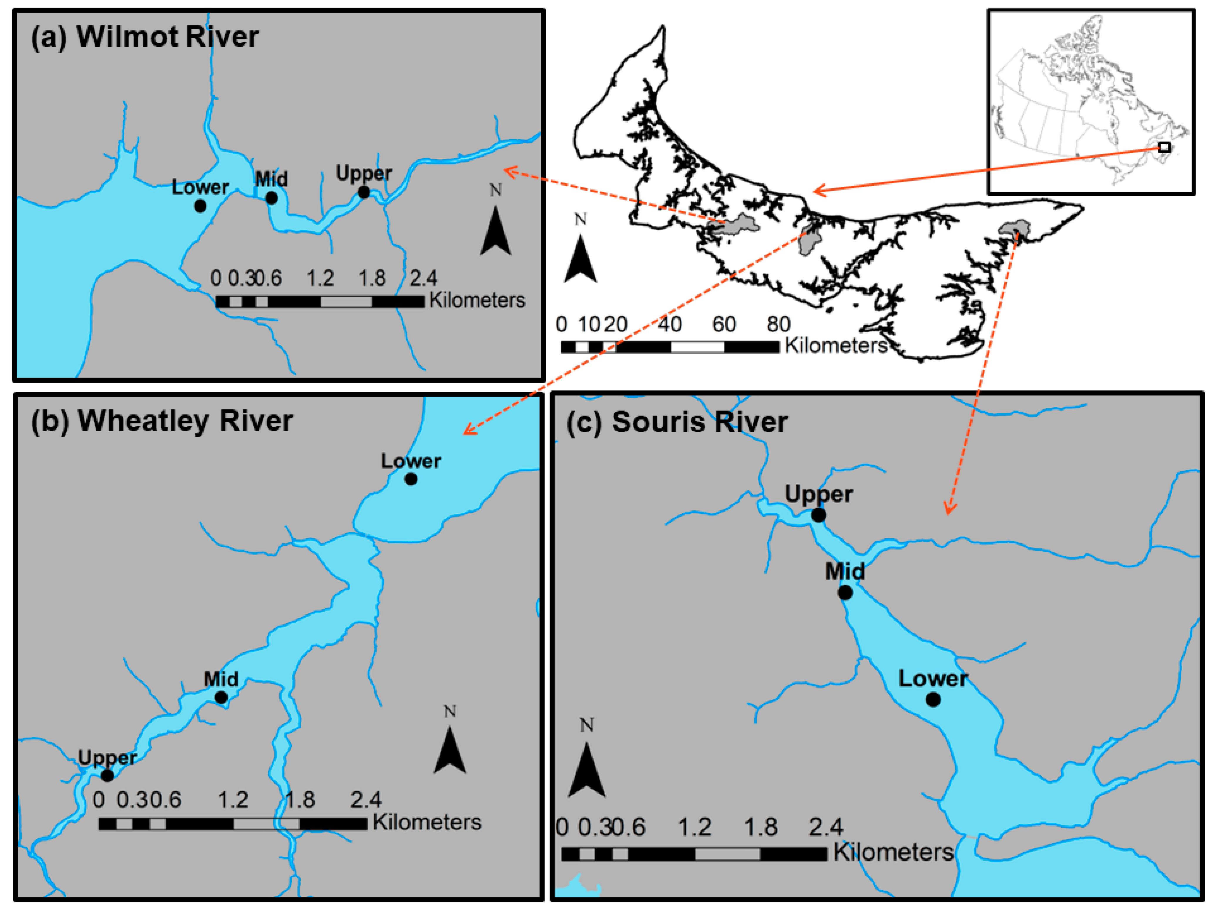
2.1. Study Location and Sampling Design

Amphipod sampling in the southern Gulf of St. Lawrence occurred within subtidal water along the coast of Prince Edward Island (PEI), Canada (Figure 1). The lithology underlying the southern Gulf of St. Lawrence differs from nearby regions, with its bedrock predominantly composed of erodible sandstone from Carbo-Permian deposits overlain with glacial till [31,32]. Remnants of the Laurentide ice sheet retreated from PEI ~10,000 years before the present [33]. Regional estuary morphometries include microtidal funnel-shaped drowned rivers or bar-built types [1,34]. PEI estuaries are generally well mixed due to relatively small river discharges that create relatively abrupt transitions from fresh to polyhaline salinities [16].
Row crop agriculture is the dominant land use and nutrient source in the drainage area of PEI estuaries (Table 1). Widely separated drainage basins with >30% agricultural land cover were selected to compare species-specific abundance patterns between estuary zones and collection methods. Runoff and the infiltration of agricultural fertilizers result in sheets of green macroalgae, primarily Ulva spp., that cover upper and mid estuary zones, whereas the seagrass, Zostera marina L., may be present in lower portions of eutrophic PEI estuaries [6,35]. Adjacent intertidal areas of PEI estuaries are typically bare sediment due to winter ice scour, but free-floating macroalgae may move throughout the estuaries [6,16].
Geomorphometry and salinity (practical salinity units, PSU) were the basis of the sampling zones within each estuary. Site selection occurred at high tide between 1 and 15 June 2016 by measuring salinities with a YSI V2 6600 multi-parameter sonde (Yellow Springs, OH, USA) at 25 cm above the benthos. The uppermost sampling zones in each estuary (Upper) occurred where the estuary funnels transitioned into river channels and were mesohaline at high tide (Figure 1). Mid-estuary sites occurred at sites with salinities ~20 PSU and were located approximately at the boundary line delimiting the inland locations of 10% of the estuary areas, as previously defined in these estuaries by Coffin et al. [1,13]. Lower estuary sites occurred at approximately 50% of the estuary areas, as in Coffin et al. [13], and were characterized by salinities of 25 PSU (Figure 1). This study considers the 10% area zone to be a midpoint of the transition from river to ocean, whereas in previous work in these three estuaries, this middle zone was the most inland point sampled and was considered the upper zone [1,13,16].
Two weeks before amphipod sampling within each zone, four sampling equipment anchors were linearly placed by boat across the estuary. The anchors were placed ~10–20 m apart at a depth of 0.5 m to <1.5 m with two 30 cm tall cement blocks tethered to a marker buoy. Sampling occurred between 5 and 9 July 2016 (Figure 1). This sampling time was chosen for the expected generalized peak in abundance of the four Gammarus species, e.g., Refs. [1,30,36].
Four euryhaline Gammarus species are common in the soft-bottom estuaries of the southern Gulf of St. Lawrence [1,29,31]. With the resources available in an estuary, Gammarus amphipods are typically omnivores and may function as detritivores, herbivores, or even predators [9,37,38]. The largest species examined here, G. oceanicus, may grow to 22 mm long and occupies multiple subtidal and intertidal habitats on both sides of the North Atlantic Ocean from the Arctic and south to Maryland in North America [29,39,40]. Gammarus lawrencianus is a predominantly estuarine species that reaches up to 13 mm in length but is restricted to North America, ranging from Newfoundland and Labrador to Connecticut and New York [11,29,41]. Another ~13 mm species, G. mucronatus, is at its northern extent in the Gulf of St. Lawrence, but its range extends to estuaries and salt marshes in the Gulf of Mexico [29,42]. Finally, though widely introduced to the freshwater and estuarine systems of Europe, G. tigrinus is native to coastal areas, ranging from Labrador to Florida except for the Great Lakes, and it may grow upward of 14 mm [29,30,43].

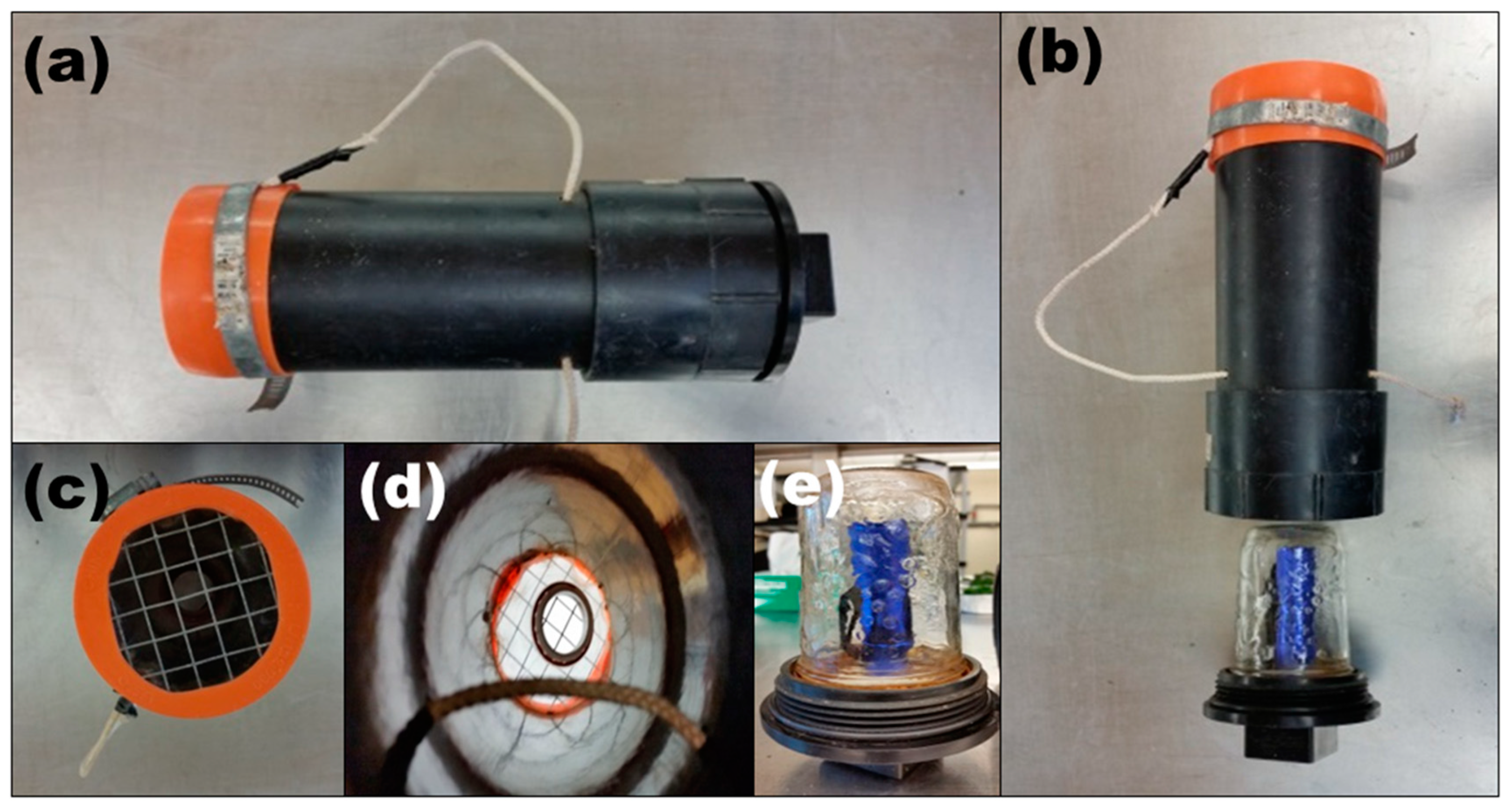
2.2. Physical Capture Equipment and Processing

Gammarus spp. collections for counts of abundance occurred in each of the three zones of each estuary, using three physical collection methods: artificial substrates, epibenthic rakes, and light-baited traps. The artificial substrate employed was a stacked plate design such as the Hester–Dendy sampler [44], with an overall surface area of the individual samplers of 0.2 m2. Five 20 × 20 cm hardboard plates were affixed with an eyebolt, nylon spacers for a 6.4 mm gap between plates, and a wingnut. The eyebolt was cable-tied to rope atop the anchoring blocks (n = 4, per site). Artificial substrates were deployed for two weeks, after which they were recovered by boat, placed into a dry tub, taken apart, and the amphipods were picked and scraped off the plates and preserved in 95% ethanol for later morphological identification.
Rake sampling occurred at a systematic random location ~10 m from each of the four sampling anchors (n = 4 per site). The epibenthic raking of macrophytes was described in detail in Coffin et al. [1,16]. However, a pivot bolt was affixed to the top of the rake doweling, and a rope was added in between the same two bow-headed rakes to standardize the area raked to 0.25 m2. From a boat, the rakes were lowered to the benthos in an extended position, closed, and brought back to the surface. The material was placed in a container. Invertebrate preservation and plant and algal matter processing and drying were as described in Coffin et al. [16] for all organic material to achieve a final count of each Gammarus spp. per gram of the total macrophyte biomass. For biomass estimates, the overall living and deceased macrophyte mass within each rake sample was utilized without separating the macrophyte species; however, dominant vegetation types were noted at each site.
The light traps were constructed of a pipe holding a light source and a funnel entrance (Figure 2). The funnel trap, or tube trap (sensu [18]), was made from the top end of a 2 L clear beverage container, 102 mm acrylonitrile butadiene styrene (ABS) piping of 20 cm length, and a 102 mm ABS screw cap. One-centimeter steel mesh was affixed to the incurrent end of the pipe and tensioned with a hose clamp, and 102 mm orange pipe caps were used with a hole cut into the pipe cap to limit incursion from non-target taxa. The light source consisted of a 19-lumen (manufacturer-specified) white-light-emitting diode (LED) flashlight with nine diodes. The flashlight was waterproofed and housed within a 739 mL clear glass jar with a 100 mm diameter complete with a size-appropriate seal and a ring lid, with the ring lid glued into the ABS screw cap (like [20]). White LEDs emit light within the 400–750 nm spectrum, but they will generally have an intensity peak within 500–600 nm, which is within the maximum absorbance range of the opsins in crustacean eyes [45,46], but was not directly measured here.
The light traps (Figure 2) were affixed to three of the four anchoring blocks using an integrated rope and cable ties ~30 cm above the substrate. They were retrieved after 24 h. The trap captures were removed by rinsing the contents onto a 500 µm sieve, with individual amphipods picked from the sieve and preserved in 95% ethanol for later counting and identification. The catch per unit of effort (CPUE) represents the counts per trap over the deployment period.
All Gammarus spp. were identified morphologically, primarily using the characters in Bousfield [29]. Physical specimen collections were processed in their entirety under a dissecting microscope using 40× magnification. Subsampling was used for samples with estimated Gammarus abundances >1000 individuals by evenly distributing the specimens on a gridded square dish and randomly subsampling 1/3 of squares and multiplying the average number of individuals per species per square by the total number of squares to estimate the total abundance per species within a sample. Species identities were verified using the molecular methods outlined below.

2.3. Sediment Collection and Analysis

For analysis of eDNA and organic matter from each site, sediment was collected in triplicate (n = 27 total: 3 estuaries × 3 sites × 3 samples) using a Mini-Ponar benthic grab in between station blocks. Benthic sediment within an intact grab was collected and stored in a 240 mL jar covered in aluminum foil, placed in an individual zip-sealed bag, and frozen at −20 °C before DNA extraction and ignition. The sediment was measured as part of method development to explore whether levels within individual samples related to DNA quantities as PCR inhibitors could be introduced from organic matter [28]. The organic matter was separately estimated through the loss on ignition technique (LOI), as described by Heiri et al. [47]. The sediment was thawed and oven-dried in a PRECISION Economy Incubator at 60 °C for 48 h and weighed. The organic matter within the sample was then combusted in an Isotemp® Programmable Muffle Furnace by heating it to 550 °C in ceramic crucibles for 4 h, cooling it to room temperature, and reweighting it to determine the relative mass of the sample organic matter. DNA was extracted separately from organic matter subsamples via a MO BIO Laboratories, Inc. (Carlsbad, CA, USA), Power Soil Kit from 0.25 g of surface sediment (~1 cm) as per the manufacturer’s instructions. The eDNA yield of each sample was determined with a NanoVue Plus microvolume spectrophotometer. The extracted DNA was stored at −20 °C.

2.4. Species-Specific Assay Design

Cytochrome oxidase 1 (COI) sequence data for the four target Gammarus species and related species from other coastal habitats were screened for nucleotide mismatches during primer design. Tissues from two PEI specimens for each of the four target species were submitted to the Canadian Center for DNA Barcoding in Guelph, Ontario, for sequencing [48]. Sequencing was successful for G. lawrencianus and G. oceanicus, with their respective sequences used in the primer design deposited in BOLD [49]. Sequences for the remaining target species were downloaded from GenBank (https://www.ncbi.nlm.nih.gov/genbank/, accessed on 20 September 2020); these included G. mucronatus (GenBank: GQ341775) and G. tigrinus (GenBank: MK403734). Related species used for screening which were less likely to occur in the soft-sediment sampling zones of the PEI estuaries included G. duebeni Lilljeborg, 1852 (GenBank: MG318075), G. setosus Dementieva, 1931 (GenBank: GQ341856), Echinogammarus finmarchicus (Dahl, 1938) (GenBank: MG320202), Marinogammarus obtusatus (Dahl, 1938) (GenBank: GQ341805), and Relictogammarus stoerensis (Reid, 1938) (GenBank: AY926657). The sequences were aligned using ClustalW and visualized using Bioedit software [50]. Variable regions of the COI gene were screened for candidate primer regions. Possible primers were generated using Primer-Blast, with the parameters set to maintain the amplicon length between 110 and 160 bp, the Guanine–Cytosine content between 20 and 80%, and the in silico melting temperatures between 58 °C and 60 °C [51]. Penultimate primers were screened through the Basic Local Alignment Search Tool (BLAST, http://blast.ncbi.nlm.nih.gov/Blast.cgi, accessed on 5 October 2020) to determine species specificity [52]. Final primer mismatches in the primer-binding region of the COI gene included 11–17 nucleotide mismatches for G. lawrencianus, 11–19 mismatches for G. mucronatus, 10–18 mismatches for G. tigrinus, and 8–15 mismatches for G. oceanicus. The chosen primers are shown in Table 2. The final COI primer regions for G. lawrencianus are an exact in silico match to G. annulatus Smith, 1873 (GenBank: AY926668), an offshore pelagic species that inhabits the Georges Bank and Nantucket Shoals [29,53]. Costa et al. [54] suggested that further systemic work is needed to clarify the relationship between nominate G. lawrencianus and G. annulatus.
DNA extraction for specificity testing followed Walsh et al. [55], using a Chelex 100 chelating resin for the tissues of each species. Each primer pair, with oligos obtained from integrated DNA Technologies, Inc. (IDT; Coralville, IA, USA), was assayed with the DNA extracts of G. lawrencianus, G. mucronatus, G. oceanicus, and G. tigrinis to ensure that they would only amplify their target species.

2.5. qPCR

The analysis was conducted using a Bio-Rad CFX96 Connect real-time PCR thermocycler (Hercules, CA, USA). The 10 µL reaction mixture consisted of 5 µL of Brilliant III Ultra-Fast SYBR Green RT-PCR master mix, with 10 µmol of forward and reverse primers (0.1 µL), 2.3 µL of nuclease-free water, 2.5 µL of DNA template, and 0.1 µL of 1% bovine serum albumin in nuclease-free water. Each run’s negative controls contained 2.5 µL of nuclease-free-water-absent template. The tissue-derived DNA in the nuclease-free water was amplified in triplicate, as below, with annealing temperatures of 54 °C to 63 °C to determine the optimal assay parameters for each of the four species and was used in remaining species-specific amplification (Table 1). The qPCR thermal profile for all samples was 95 °C for 3 min, then forty cycles of 95 °C for 5 s, a species-specific annealing temperature for 15 s, and then 72 °C for 1 min. A melt curve was determined per sample for reaction specificity. A subset of eDNA and tissue amplifications for each species was reamplified using species-specific qPCR assays to increase the DNA concentrations for Sanger sequence verification. Target sequences were bidirectionally verified using an Applied Biosystems™ 3730xl DNA Analyzer (Waltham, MA, USA) at Genome Quebec, Montreal, QC, Canada, using the species-specific primers in the Sanger reaction (Figure S1).
Aliquots of the 27 eDNA samples were amplified with the four species-specific primer pairs in singleplex reactions. Each eDNA sample was diluted by a factor of 10 to limit non-specific binding. Technical replicates of each eDNA sample were in quintuplicate, with mean values retained for quantitative comparisons. Quantities of DNA were compared to a 5-fold dilution standard curve for each species on each plate. The copy number was determined by comparing the standard curves to 7-fold dilutions of 499 bp artificial gBlock DNA for each species (IDT; Table 1). Each species’ gBlock contained the intended COI fragment at its center and was based on the primer design sequences.

2.6. Statistical Analysis

The analysis comparing the related species among estuary locations and sampling methods employed an alpha of 0.05 using R function packages [56] and PRIMER-e Version 7 with PERMANOVA + software, version 7.0.17 [57,58].
Spatial hypotheses were examined through generalized linear mixed models (GLMM) in R. Due to differences in the response data types among the absolute abundance indicators, individual species counts or eDNA concentrations were regressed separately against site-selection salinity measurements to examine if the same spatial conclusions were reached per species–method GLMM model. The GLMMs for Gammarus counts assumed a negative binomial error and log-link, whereas the continuous eDNA concentration analysis used gamma errors and a log-link within lme4 package routines [59]. The normality of residuals and the homogeneity of variance were visually examined using quantile–quantile plots and plotting residuals against fitted values respectively. Residual dispersions for all models were examined via dividing the Pearson Chi-square statistic by the model’s degrees of freedom. Within the raking samples, vegetation biomass was an offset factor in each of the species models. Sampling replicates were nested within each sampling site. The estuary, as a hierarchal factor, was removed in the analyses for all species as either estuary-level random effects correlated with the sampling site (a lower factor) in a preliminary analysis or the preliminary 95% confidence intervals per estuary overlapped [59]. Fits of the mixed models were determined using the log-normal R2 from the package MuMIn [60]. The marginal R2 (Rm2) describes the fit of the spatial parameter, salinity, and the conditional R2 overall mixed-effect model fit (Rc2). Any method for which there were <15 total individuals across estuaries was not modeled for spatial abundance questions but was compared in a further analysis.
The remaining univariate method or sample comparisons considered the strength of the association through the Pearson correlation (r) for interpretation. Sample-level correlations used measured values. Site-level correlations among species counts and DNA concentrations used the means of the measured values within each zone, method, and estuary for comparison.
To understand the multi-species effects of the habitat zone and collection method groupings, comparisons among species were standardized using the total Gammarus in samples for a multivariate analysis. The proportion data of each species total among the total Gammarus spp. in a sample were square-root transformed. Distances between samples used a Gower dissimilarity matrix as only four species are in the matrix. For comparisons of the assemblage between and within estuaries, the method and estuary were treated as fixed factors with samples nested within the zone. Multi-species comparisons used a permutational multivariate analysis of variance (PERMANOVA) with main effects and the paired contrast p-values generated through Monte-Carlo resampling and simulated 9999 times using the same dissimilarity matrix within the PERMANOVA + addon to PRIMER-E. The homogeneity of the multivariate dispersion (PERMDISP) between factors was compared permutationally within the PERMANOVA +. The multivariate distance visualizations between sites were generated using non-metric multidimensional scaling (nMDS) plots through the R package Vegan [61].

3. Results

3.1. Habitat Conditions

The spatial sampling gradient resulted in salinity and sediment organic matter varying with increasing distance from the ocean, though there are other habitat differences between the estuaries (Table 3). Overall, salinities were the highest in the Souris estuary and lowest in the Wilmot estuary. Along the spatial gradient, the overall differences from the upper to outer zones were the highest within the 4.1 km of the Wheatley, followed by the 2.3 km of the Wilmot, and the lowest was in the 2.1 km of the Souris. The loss on ignition (LOI)-derived sediment organic matter declined from the upper to the outer sites in both the Souris and Wheatley, with the highest sediment organic matter occurring at the mid site in the Wilmot. The highest raked macrophyte biomass within each estuary occurred in different zones, with the lower zone of the Wilmot being four times higher than the mid, the mid zone of the Wheatley being two times higher than the lower, and the upper zone of the Souris being two times higher than the mid.

3.2. Physical Sampling Summary and Occupancy

Across all sites and physical methods, the total Gammarus spp. captured amounted to 14,055 individuals. Among the total physical collections, 59.8% of the individuals originated from light-baited traps, 21.3% from artificial substrates, and the remainder came from epibenthic raking. Across the methods and estuaries, 80.9% of individuals were collected at the upper sites, with 7.1% at the mid sites and 11.4% at the lower sites. Among estuaries, 68.8% of the total Gammarus spp. were from the Wheatly estuary, 26.3% were from the Souris estuary, and the fewest overall captures were from the Wilmot estuary (Table 4). No Gammarus spp. were collected in the lower Souris raking or in Upper Wilmot artificial substates. Light traps always detected the presence of at least one species across zones and estuaries (Table 4). In contrast, the light-baited traps failed to capture any G. oceanicus in the Souris estuary, where its presence was found by using the other physical methods (Table 4). Finally, no G. tigrinus was collected in the Souris estuary using any physical collection method. The majority of the individuals of this species collected in other estuaries came from upper samples (Table 4).

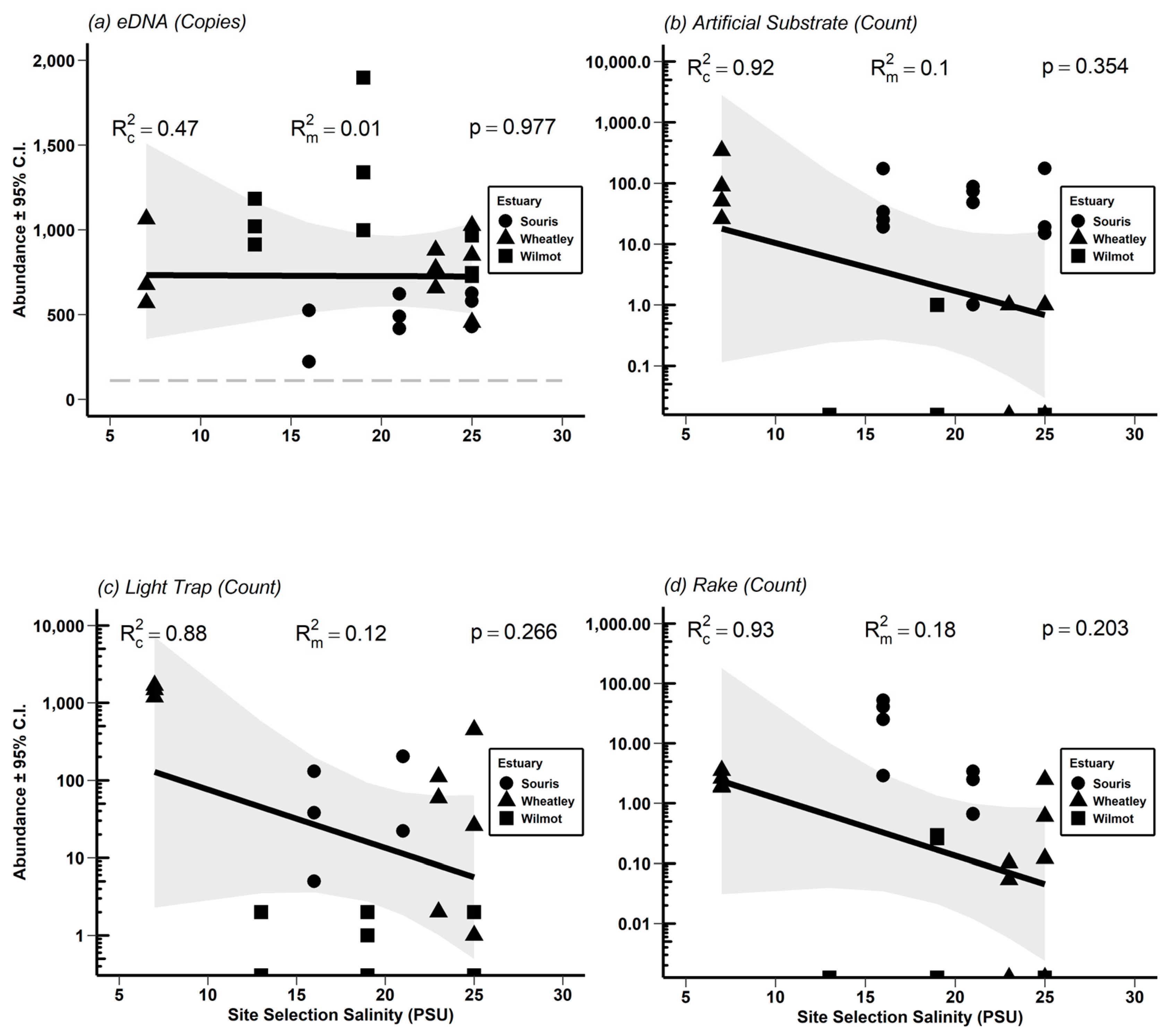
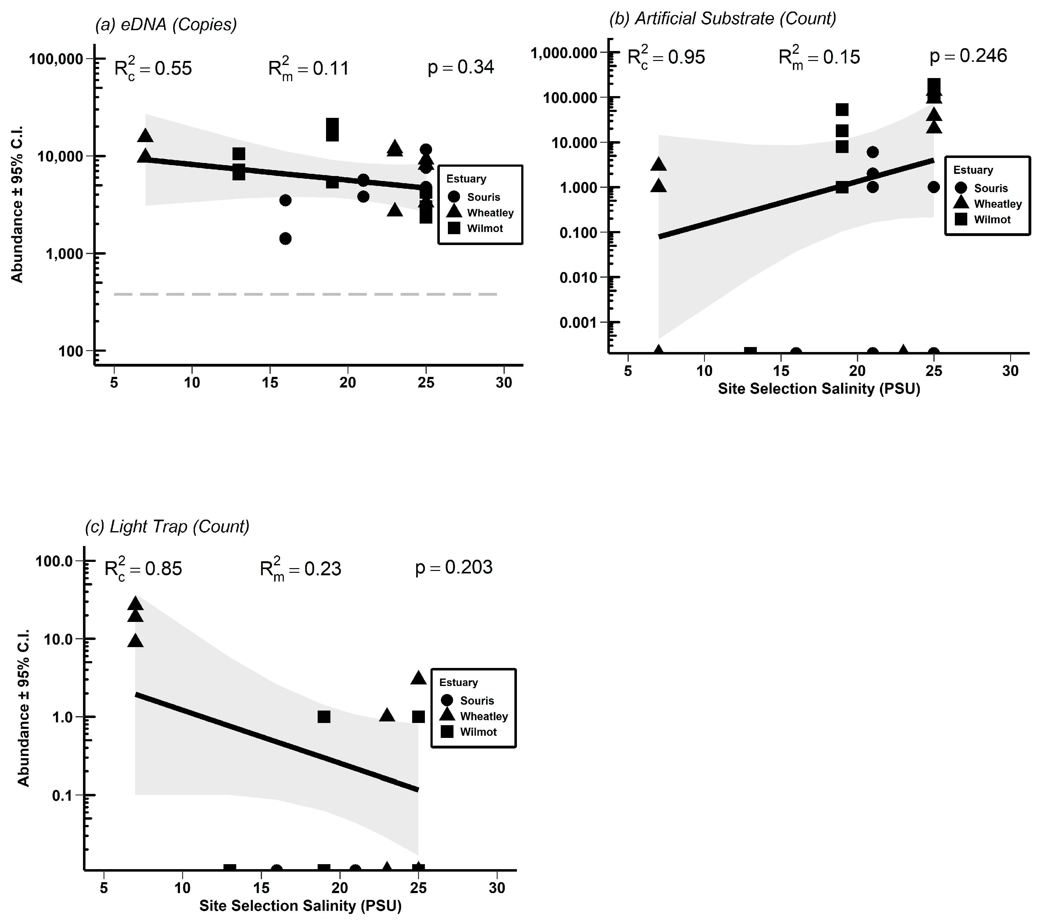
3.3. Absolute Abundance Gradients and Comparison of Physical Methods to eDNA

The change in abundance along the sampled spatial gradient was clear for only G. mucronatus. Irrespective of the physical collection method used, counts of G. mucronatus significantly declined with increasing site-selection salinity (Figure 3). Similarly, abundances declined with increasing salinity for G. lawrencianus when using all physical collection methods; however, these relationships were not statistically significant (Figure 4). Likewise, there was no significant effect of salinity on any abundance indicator of G. oceanicus, though counts on artificial substrates increased with higher salinities, and catches decreased with higher salinities in the light traps (Figure 5). Unlike physical techniques, the abundances inferred from eDNA did not significantly change across the salinity gradient for any species (Figure 3, Figure 4, Figure 5 and Figure S2).
Correlations between the mean estimates of the species’ absolute abundances per zone across the estuaries are outlined in Table 5 and visualized in Figure S3. All methods used provided comparable abundance trends between the sampling sites for G. mucronatus as all mean estimates by zone are positively correlated, though the correlations are weakest between the eDNA and physical collection methods. By comparison, the abundance indicators for G. lawrencianus only weakly (non-significantly) correlated between physical collections, and the eDNA estimates demonstrate the opposite trend of abundances from the mean physical collections. Average copies of G. lawrencianus eDNA in the Wilmot estuary were marginally higher than in the other systems, whereas counts of this species were always the lowest in the Wilmot using any physical method compared to the other systems (Figure 4). For G. oceanicus, only raking and light-trap sampling yielded weakly (non-significantly) comparable estimates of local-scale abundance trends. However, as each method accumulates different totals among the Gammarus spp. (Table 4), standardized contrasts of each species’ relative abundances were compared via a multivariate analysis.

3.4. Multivariate Examination of Gammarus Assemblage between Zones and Methods

The assemblage structures of the Gammarus spp., examined using multivariate statistics, changed between the zones and similarly across the sampled estuaries (Figure 6). The Gammarus spp. assemblage centroids from the Gower dissimilarity were significantly different between estuary zones and between the physical collection methods used (PERMANOVA). Paired contrasts of the main effects of sampling location between the upper, mid, and lower sites indicate that the sampling zone assemblages were significantly different from each other across methods and estuaries (PERMANOVA). Relative percentages of the individual species change between zones along the estuary sampling gradient (Figure 6), with G. mucronatus or G. lawrencianus being dominant in upper zones, and G. oceanicus being dominant in lower estuaries (Table 3). Paired contrasts indicate similar overall Gammarus spp. assemblages between the artificial substrates and light-baited traps; likewise, the main-effects centroids between the artificial substrate and raking samples were not significantly different across zones and estuaries (PERMANOVA). However, contrasts of the light-trap assemblage significantly differed from the raking assemblage (PERMANOVA; Figure 6). Environmental DNA was not included in the multivariate analysis as species-specific qPCR assays do not allow for the standardization of total copies among the four separate assays.
There was no statistical interaction between method and estuary, but there were assemblage differences between estuaries (Table S3). Between estuaries, the overall Gammarus spp. assemblages were significantly different among all methods and locations (PERMANOVA, Figure 6). Pairwise contrasts of estuary-specific centroids showed significant differences in Gammarus assemblages only between the Souris and Wilmot estuaries (PERMANOVA; Figure 6). For example, G. oceanicus is rare in the Souris estuary (Table 3). The multivariate dispersion differed between estuaries (across methods and locations), with the dispersions in Souris significantly less variable than the other two estuaries (PERMDISP contrast, Figure 6).
There were method-specific differences in species percentages within individual sampling zones. The overall PERMANOVA indicated a significant interaction between zone and method, suggesting that zonal effects can be method-specific (Tables S3 and S4). Where there was a significant zone–method interaction between light traps and raking, there was a substantially higher fraction of G. mucronatus in raking samples vs. light traps, with the opposing pattern found for G. lawrencianus, which dominated light traps in these locations (Table 4). The observed assemblages were significantly different between raking and substrates in the lower zone of every estuary (PERMANOVA; Table S5). The zone–method interaction between raking and substrate collections was explained by the dominance of G. oceanicus on artificial substrates and the relative absence of this species in raking samples (Table 4). The PERMDISP analysis showed an even multi-species dispersion between the zones and methods overall.

4. Discussion

Gammarus species abundance changes were evident along the river-to-ocean transition but required multiple methods of physical capture to elucidate. The abundance of G. mucronatus was the highest in the upper estuary and declined with increasing salinity. G. lawrencianus were prevalent across zones, though their abundance only decreased modestly along the salinity-sampling gradient when compared to G. mucronatus. Intermittent occurrences of G. tigrinus were only observed in the less saline regions, and the proportions of G. oceanicus were most prevalent in lower, more saline estuary zones on artificial substrates. In contrast to the physical methods, sediment eDNA could not detect any linear species-specific abundance effects spatially, and the only species for which the copy number positively correlated with average counts was G. mucronatus.
Species replacement/turnover along salinity gradients is an expected community feature along larger estuaries and is related to the origin and environmental adaptation of the Gammarus species [4,10,62]. Though there is often overlap in occurrence among Gammarus species along coastal gradients [8], there are spatial differences in the abundances and proportions of Gammarus spp. in small estuaries, including those in PEI. Saline Gammarus in North America diverged from marine Eurasian clades in the Paleocene [62], suggesting convergence in resultant speciation patterns under similar gradient pressures [12,63]. Repeated contemporary introductions of the North-American-origin G. tigrinus occur in oligohaline and freshwater areas in Europe, matching their overall native range [10,43] and rare occurrences in mesohaline zones herein. On the opposite end, G. oceanicus is of a Palearctic origin but entered North America before the last interglacial period [62,64]. Across the Atlantic, there are frequent reports of higher occupations of G. oceanicus in the outer areas of estuaries [39,40], including high proportions on the lower-zone artificial substrates herein. Laboratory studies exposing G. oceanicus to multiple salinities confirmed this fundamental niche parameter through the observed marginally higher survival and reduced energy expenditure at ≥30 PSU [10,65]. However, the survival of G. oceanicus appears to be primarily limited by freshwater; this broad salinity tolerance may explain why absolute counts of this species did not increase with increasing ocean influence but the relative abundance did [10].
Both G. mucronatus and G. lawrencianus are estuary resident species [1,11], but their abundance and prevalence patterns relate to specific sections of estuaries. In experimental exposures of G. lawrencianus to salt levels between 2.5 and 35 PSU, survival was highest within the 15–25 PSU range [41]. However, growth and reproductive endpoints did not change between 15 and 35 PSU [41]. This wide range of salinity supports a predominant lack of changes in abundance across the sampled salinity range in the present study and the generally high proportions across the estuarine zones of PEI. Unfortunately, there are no similar salinity exposures to help explain the stronger pattern of G. mucronatus abundance with the salinity gradient, and these results can only be compared to those from other estuaries. Quantitative studies along subtidal gradients are rare for estuaries containing G. mucronatus [11]; however, contrary to the present study, the abundance of G. mucronatus did not change along a salinity gradient in a single Connecticut estuary [66]. However, the G. mucronatus biomass was the highest in a Chesapeake Bay seagrass bed in years that had average salinities of between 14 and 20 vs. >20 PSU [37], potentially suggesting an adaptation to a lower level of salinity. Likewise, G. mucronatus can be found as the dominant macroinvertebrate species in oligohaline zones of Alabama [42], which is generally consistent with the upper and mid-zone raking samples assessed herein.
Resource availability along estuaries also influences species zonation [6,35]. Though vegetation types were not separated for the raking biomass estimates, eelgrass patches were only observed near lower zones, with the green macroalgae Ulva dominating in the upper to mid areas. These conditions are consistent with previous surveys of eelgrass or Ulva cover in eutrophic estuaries across the southern Gulf of St. Lawrence [6,35]. In addition more red and brown macroalgae diversity is typically found as one approaches the ocean [17,67]. Indeed, G. oceanicus feeds on marine red macroalgae in an outer estuary area of PEI, but may also consume marine bivalve tissue [17,65]. Laboratory feeding trials suggest that G. lawrencianus will consume green macroalga, a variety of filamentous marine red, and brown algae [38]. However, it remains unclear what G. lawrencianus consumes in upper-mid estuaries. The diets of the upper-estuary Gammarus spp. in PEI and Massachusetts are isotopically linked to Ulva mats and associated detritus [7,36]. Experimentally, G. mucronatus preferentially feeds on Ulva spp. over multiple red algal species and is linked isotopically to multiple green macroalgae and periphyton [68,69]. Lastly, Gammarus are generally omnivorous, and intraguild predation among different Gammarus species may reinforce species zonation in estuaries [9]; however, nitrogen isotope evidence of PEI Gammarus feeding at higher tropic levels is largely lacking [7].
Competition for space among Gammarus species explains artificial substrate patterns. G. oceanicus often selects more structurally complex microhabitats [14,70], potentially leading to dominance in the lower zone artificial substrates if the physically smaller Gammarus species are expelled locally [29,40]. In a Quebec intertidal eelgrass meadow, G. oceanicus was only found among structurally complex eelgrass, whereas G. lawrencianus densities were 3 to 7-fold higher in adjacent ice-scoured pools at low tide [14]. Likewise, in a similar ice-scour experiment in Nova Scotia, the absolute abundances of G. mucronatus were positively correlated with a less-complex macroalgae biomass that colonized scoured areas and negatively correlated with eelgrass biomass [71]. For benthic treatments of red macroalgae and mussels in the outer area of another PEI estuary, G. oceanicus are the dominant species among branching fronds of Chondrus crispus Stackh., and G. oceanicus make up three-quarters of the amphipods in mixtures of C. cripsus and Mytilus edulis Linnaeus, 1758 [17], supporting the multivariate artificial substrate patterns observed herein. Nevertheless, the degree of direct interactions among coastal Gammarus are species- and substrate-dependent [8,40].
Species-specific behavior toward nocturnal light cues affects light-trap captures [18,21,45]. G. oceanicus were infrequent in light-baited traps, indicating limited nocturnal phototaxis. Freshwater Gammarus species in Europe, which are more closely related to G. oceanicus [62], appear to not alter their behavior when exposed to artificial light at night [21,45]. The eye of G. oceanicus has ultrastructure adaptations for low light; however, it maintains its function under the 24 h light of the Arctic [72]. Founding populations of North American G. oceanicus may have traversed areas with limited dark periods to their present range, suggesting the potential for little reliance on nocturnal light cues [11,64]. In contrast, most light-trap captures were the species G. mucronatus and G. lawrencianus. Closely related to G. lawrencianus [54], G. annulatus has adopted a divergent pelagic life history and is more frequently captured during night trawls despite having similar day/night abundances [53,73]. Likewise, G. lawrencianus are more prevalent in light-trap samples relative to raking, but this effect is zone-dependent. Nevertheless, shallow-water G. tigrinus abundances above the benthos are the highest at night [15], corresponding with the larger number of individual amphipods captured by light traps in our study.
Environmental DNA persistence or transport dynamics in sediment explain the lack of spatial relationships between the eDNA copy numbers and the counts achieved with the physical collection methods. The expectation was that amphipod sediment eDNA copies would correspond to physical abundance estimates at each site; however, these types of correlations for amphipods may only be detectible during the initial phase of eDNA degradation in surface sediments [22,28]. Degradation rates are usually slowest for smaller eDNA fragments, especially from sediment, which subsequently influences whether quantitative relationships can be found with species abundance [22,24,28]. Thus, the site-level correlation of eDNA with counts for G. mucronatus may relate to this species’ assay having smallest species-specific fragment. Indeed, more recent eDNA metabarcoding for arthropod species presence/absence from PEI estuaries suggests that sediment eDNA along estuary gradients are homogeneous for overall diversity, whereas aqueous eDNA sampling may allow for the differentiation of salinity-related biodiversity patterns [74]. Nevertheless, metabarcoding for invertebrates from aqueous eDNA along a German estuary suggests that oceanic faunal DNA are transported with the tide [75]. Likewise, in rivers, quantities of crustacean eDNA can change with the distance from the source population [23,76]. These DNA transport phenomena, combined with the longevity of DNA in sediment, could contribute to the G. mucronatus eDNA patterns found herein, with a marginal decline in copies relative to the distance from the abundant upper population sources [76]. For G. lawrencianus, the negative relationship of eDNA to local counts may reflect transported DNA from outer zones that were not sampled through tidal forces rather than river flow [23,75], as overall salinities in the Wilmot estuary and the counts of this species there were lowest overall. The influence of bidirectional tidal flow, water residence, and estuary depositional patterns also remain unclear for estuary eDNA amounts as there is a dearth of studies in brackish systems and on aquatic arthropods in general [27,75,77].
Species-specific indicators of abundance or assemblage dominance should respond in the same manner between estuarine sites when using different monitoring methods [1,5]. Univariate analysis did not show clear differences in abundances between individual estuaries but did point to the important role of the salinity gradient within estuaries. Multiple methods were needed to differentiate estuaries based on Gammarus assemblages. Anthropogenic effects on biodiversity are often difficult to detect within and between estuaries due to the rapid changes in habitat conditions, including salinity [3]. Nevertheless, assemblage structure differences between the higher-tidal-amplitude Wilmot estuary and other systems were apparent with all methods combined, matching the responses of previous invertebrate assemblage monitoring that used raking alone [1]. However, raking requires both sorting and processing the macrophyte biomass, whereas substrates and traps eliminate these steps. Despite the overall assemblage structure differences between raking and light-trap collections, correlations in absolute abundance trends are positive between these two methods for all species. For G. oceanicus, there are no clear correlations between artificial substrates and the other techniques. However, G. oceanicus is a dominant species on many of the artificial substrates, highlighting that relative vs. absolute abundance responses are critical considerations in choosing an amphipod-monitoring method. The high productivity of Gammarus spp. make these species important components of coastal food webs and ideal for biomonitoring [7,53,78]. Thus, efficient means of quantification are preferable for managers to incorporate amphipod monitoring [2,5,17].

5. Conclusions

Abundance and proportion responses along sampled estuaries are method-dependent, but understanding method-specific biases is imperative for their utilization in future applied questions. Similar to assemblages of coastal Gammarus species in other regions, the species within this genus contribute to turnover along short northwestern Atlantic estuaries [4,8]. The results suggest that careful consideration of method choice or multiple methods are needed to account for typical estuarine species–environment gradients when focusing on the abundance or assembly responses of crustacean species with biomonitoring and ecotoxicological utilities [1,78]. Light-traps are recommended for Gammarus-specific or eutrophication questions as this method provided absolute abundance trends that were consistently comparable to the previously used and more resource-intensive raking methods [1,16]. Artificial substrates may be most appropriate for compositional comparisons if a single method is used. However, future mesocosm experiments involving species-specific microhabitat selection or nocturnal behaviors would aid in validating the life-history differences inferred from the different patterns among field methods. Nevertheless, future studies should explore arthropod eDNA transport dynamics within estuaries to account for quantitative differences. Likewise, to substantiate the multivariate patterns herein, future studies should examine focused-species assemblages through metabarcoding-based approaches from either bulk sample or eDNA sources [74,75,79].

Supplementary Materials

The following supporting information can be downloaded at: https://www.mdpi.com/article/10.3390/d15060714/s1, Table S1: Within-estuary and overall Pearson correlations ® between the amount of sediment-sample-level eDNA (Copy num.) and the corresponding sediment loss on ignition organic matter (OM, %), Table S2: Individual method-specific model parameters examining the relationship between absolute abundance indicators and spatial zonation among sampled estuaries, Table S3: Parameter results from PERMANOVA tests of Prince Edward Island Gammarus assemblages, Table S4: Parameter results of paired contrasts between factor groupings of Prince Edward Island Gammarus assemblages through centroids of Gower dissimilarity differences, Table S5: Parameter results of paired contrasts between interactions of factor groupings of Prince Edward Island Gammarus assemblages through centroids of Gower dissimilarity differences, Table S6: Parameter results from PERMSISP tests of Prince Edward Island Gammarus assemblages comparing grouping variance of Gower dissimilarities, Table S7: Parameter results of PERMSISP paired contrast differences between estuary variances of Prince Edward Island Gammarus assemblages through estuary-specific variability of Gower dissimilarities; Figure S1: Comparison of the reference DNA fragment sequence for species-specific assays and relative base pair position with the consensus sequences recovered from amplifying reference tissue extracts for each species and eDNA extracts from select samples, Figure S2: Non-significant gamma mixed-effects model relationship between salinity and sediment eDNA copies for G. tigrinus across sampled PEI estuaries, Figure S3: Bivariate plots of data for Gammarus spp. indicators of absolute abundance vs. site selection salinity, Figure S4: Representative post-qPCR gel highlighting fragment size differences between species assays from eDNA and tissue-based extractions.

Author Contributions

Conceptualization, K.M.K. and M.R.v.d.H.; methodology, K.M.K., C.M.G. and M.R.v.d.H.; formal analysis K.M.K.; investigation K.M.K., L.P.M. and J.M.C.; resources S.C.C. and M.R.v.d.H.; data curation, K.M.K.; writing—original draft preparation K.M.K.; writing—review and editing, K.M.K., L.P.M., J.M.C., C.M.G., S.C.C. and M.R.v.d.H.; visualization, K.M.K.; supervision, S.C.C. and M.R.v.d.H.; project administration, K.M.K. and M.R.v.d.H.; funding acquisition K.M.K. and M.R.v.d.H. All authors have read and agreed to the published version of the manuscript.

Funding

This research was funded in part by the Natural Sciences and Engineering Research Council of Canada Strategic Projects Grant (NSERC-SGTP 463277-14) to M.R.v.d.H. and a 2019 University of Prince Edward Island (UPEI) Internal Research Grant to K.M.K and M.R.v.d.H. K.M.K. was personally supported by the J. Regis Duffy Scholarship in Science, the Peter MacCormack Memorial Scholarship, the Minto and Vina Foster Graduate Scholarship in Biology, and the UPEI Faculty Association Doctoral Medal.

Institutional Review Board Statement

All organisms were handled in a manner subject to University of Prince Edward Island animal care protocols. As such, no institutional review was required for field-based study on the subject invertebrate species. All collection activities complied with a scientific license granted by the Department of Fisheries and Oceans, Canada (SG-RHQ-16-004).

Data Availability Statement

The raw data and analysis code presented in this study are available upon reasonable request from the corresponding author.

Acknowledgments

The authors would like to thank J. Kidd, C. Pater, S. Roloson, and T. James for their assistance during equipment construction and fieldwork. S. Larter and M. Kays were helpful in the preliminary development of the eDNA assays. Additionally, we would like to thank D. Giberson, S. Greenwood, R. Steeves, and M. Coffin for their helpful discussions. Finally, we thank the anonymous reviewers for their constructive criticisms that greatly improved this manuscript.

Conflicts of Interest

The authors declare no conflict of interest.

References

  1. Coffin, M.R.S.; Courtenay, S.C.; Knysh, K.M.; Pater, C.C.; van den Heuvel, M.R. Impacts of Hypoxia on Estuarine Macroinvertebrate Assemblages across a Regional Nutrient Gradient. Facets 2018, 3, 23–44. [Google Scholar] [CrossRef]
  2. Kraufvelin, P.; Salovius, S.; Christie, H.; Moy, F.E.; Karez, R.; Pedersen, M.F. Eutrophication-Induced Changes in Benthic Algae Affect the Behaviour and Fitness of the Marine Amphipod. Gammarus Locusta. Aquat. Bot. 2006, 84, 199–209. [Google Scholar] [CrossRef]
  3. Elliott, M.; Quintino, V. The Estuarine Quality Paradox, Environmental Homeostasis and the Difficulty of Detecting Anthropogenic Stress in Naturally Stressed Areas. Mar. Pollut. Bull. 2007, 54, 640–645. [Google Scholar] [CrossRef] [PubMed]
  4. Whitfield, A.K.; Elliott, M.; Basset, A.; Blaber, S.J.M.; West, R.J. Paradigms in Estuarine Ecology—A Review of the Remane Diagram with a Suggested Revised Model for Estuaries. Estuar. Coast. Shelf Sci. 2012, 97, 78–90. [Google Scholar] [CrossRef]
  5. Quintino, V.; Sangiorgio, F.; Mamede, R.; Ricardo, F.; Sampaio, L.; Martins, R.; Freitas, R.; Rodrigues, A.M.; Basset, A. The Leaf-Bag and the Sediment Sample: Two Sides of the Same Ecological Quality Story? Estuar. Coast. Shelf Sci. 2011, 95, 326–337. [Google Scholar] [CrossRef]
  6. van den Heuvel, M.R.; Hitchcock, J.K.; Coffin, M.R.S.; Pater, C.C.; Courtenay, S.C. Inorganic Nitrogen Has a Dominant Impact on Estuarine Eelgrass Distribution in the Southern Gulf of St. Lawrence, Canada. Limnol. Oceanogr. 2019, 64, 2313–2327. [Google Scholar] [CrossRef]
  7. Schein, A.; Courtenay, S.C.; Kidd, K.A.; Campbell, K.A.; van den Heuvel, M.R. Food Web Structure within an Estuary of the Southern Gulf of St. Lawrence Undergoing Eutrophication. Can. J. Fish. Aquat. Sci. 2013, 70, 1805–1812. [Google Scholar] [CrossRef]
  8. Herkül, K.; Lauringson, V.; Kotta, J. Specialization among Amphipods: The Invasive Gammarus tigrinus Has Narrower Niche Space Compared to Native Gammarids. Ecosphere 2016, 7, e01306. [Google Scholar] [CrossRef]
  9. MacNeil, C.; Dick, J.T.A. Intraguild Predation May Reinforce a Species-Environment Gradient. Acta Oecologica 2012, 41, 90–94. [Google Scholar] [CrossRef]
  10. Paiva, F.; Barco, A.; Chen, Y.; Mirzajani, A.; Chan, F.T.; Lauringson, V.; Baltazar-Soares, M.; Zhan, A.; Bailey, S.A.; Javidpour, J.; et al. Is Salinity an Obstacle for Biological Invasions? Glob. Chang. Biol. 2018, 24, 2708–2720. [Google Scholar] [CrossRef]
  11. Hunte, W.; Myers, R.A. Phototaxis and Cannibalism in Gammaridean Amphipods. Mar. Biol. 1984, 81, 75–79. [Google Scholar] [CrossRef]
  12. Wildish, D.J.; Radulovici, A.E. Amphipods in Estuaries: The Sibling Species Low Salinity Switch Hypothesis. Zoosyst. Evol. 2020, 96, 797–805. [Google Scholar] [CrossRef]
  13. Coffin, M.; Knysh, K.; Roloson, S.; Pater, C.; Theriaul, E.; Cormier, J.; Courtenay, S.; van den Heuvel, M. Influence of Nutrient Enrichment on Temporal and Spatial Dynamics of Dissolved Oxygen within Northern Temperate Estuaries. Environ. Monit. Assess. 2021, 193, 804. [Google Scholar] [CrossRef] [PubMed]
  14. Pascal, L.; Bernatchez, P.; Chaillou, G.; Nozais, C.; Lapointe Saint-Pierre, M.; Archambault, P. Sea Ice Increases Benthic Community Heterogeneity in a Seagrass Landscape. Estuar. Coast. Shelf Sci. 2020, 243, 106898. [Google Scholar] [CrossRef]
  15. Stearns, D.E.; Dardeau, M.R. Nocturnal and Tidal Vertical Migrations of “benthic” Crustaceans in an Estuarine System with Diurnal Tides. Northeast. Gulf Sci. 1990, 11, 93–104. [Google Scholar] [CrossRef]
  16. Coffin, M.R.S.; Knysh, K.M.; Theriault, E.F.; Pater, C.C.; Courtenay, S.C.; van den Heuvel, M.R. Are Floating Algal Mats a Refuge from Hypoxia for Estuarine Invertebrates? PeerJ 2017, 5, e3080. [Google Scholar] [CrossRef]
  17. Tummon Flynn, P.; Lynn, K.; Cairns, D.; Quijón, P. Mesograzer Interactions with a Unique Strain of Irish Moss Chondrus crispus: Colonization, Feeding, and Algal Condition-Related Effects. Mar. Ecol. Prog. Ser. 2021, 669, 83–96. [Google Scholar] [CrossRef]
  18. McLeod, L.E.; Costello, M.J. Light Traps for Sampling Marine Biodiversity. Helgol. Mar. Res. 2017, 71, 2. [Google Scholar] [CrossRef]
  19. Navarro-Barranco, C.; Irazabal, A.; Moreira, J. Demersal Amphipod Migrations: Spatial Patterns in Marine Shallow Waters. J. Mar. Biol. Assoc. U. K. 2020, 100, 239–249. [Google Scholar] [CrossRef]
  20. Hungerford, H.B.; Spangler, P.J.; Walker, N.A. Subaquatic Light Traps for Insects and Other Animal Organisms. Trans. Kansas Acad. Sci. 1955, 58, 387–407. [Google Scholar] [CrossRef]
  21. Czarnecka, M.; Grubisic, M.; Kakareko, T. Disruptive Effect of Artificial Light Light at Night on Leaf Litter Consumption, Growth and Activity of Freshwater Shredders. Sci. Total Environ. 2021, 786, 147407. [Google Scholar] [CrossRef] [PubMed]
  22. Wei, N.; Nakajima, F.; Tobino, T. Variation of Environmental DNA in Sediment at Different Temporal Scales in Nearshore Area of Tokyo Bay. J. Water Environ. Technol. 2019, 17, 153–162. [Google Scholar] [CrossRef]
  23. Rice, C.J.; Larson, E.R.; Taylor, C.A. Environmental DNA Detects a Rare Large River Crayfish but with Little Relation to Local Abundance. Freshw. Biol. 2018, 63, 443–455. [Google Scholar] [CrossRef]
  24. Wei, N.; Nakajima, F.; Tobino, T. Effects of Treated Sample Weight and DNA Marker Length on Sediment eDNA Based Detection of a Benthic Invertebrate. Ecol. Indic. 2018, 93, 267–273. [Google Scholar] [CrossRef]
  25. Crane, L.C.; Goldstein, J.S.; Thomas, D.W.; Rexroth, K.S.; Watts, A.W. Effects of Life Stage on eDNA Detection of the Invasive European Green Crab (Carcinus maenas) in Estuarine Systems. Ecol. Indic. 2021, 124, 107412. [Google Scholar] [CrossRef]
  26. Trimbos, K.B.; Cieraad, E.; Schrama, M.; Saarloos, A.I.; Musters, K.J.M.; Bertola, L.D.; Bodegom, P.M. Stirring up the Relationship between Quantified Environmental DNA Concentrations and Exoskeleton-shedding Invertebrate Densities. Environ. DNA 2020, 3, 605–618. [Google Scholar] [CrossRef]
  27. Andruszkiewicz Allan, E.; Zhang, W.G.; Lavery, A.; Govindarajan, A. Environmental DNA Shedding and Decay Rates from Diverse Animal Forms and Thermal Regimes. Environ. DNA 2021, 3, 492–514. [Google Scholar] [CrossRef]
  28. Wei, N.; Nakajima, F.; Tobino, T. A Microcosm Study of Surface Sediment Environmental DNA: Decay Observation, Abundance Estimation, and Fragment Length Comparison. Environ. Sci. Technol. 2018, 52, 12428–12435. [Google Scholar] [CrossRef]
  29. Bousfield, E.L. Shallow-Water Gammaridean Amphipoda of New England; Comstock Publishing Associates Cornell University Press: Ithaca, NY, USA, 1973; p. 312. [Google Scholar]
  30. Steele, D.H.; Steele, V.J. The Biology of Gammarus (Crustacea, Amphipoda) in the Northwestern Atlantic. XI. Comparison and Discussion. Can. J. Zool. 1975, 53, 1116–1126. [Google Scholar] [CrossRef]
  31. Bousfield, E.L.; Thomas, M.L.H. Postglacial Changes in Distribution of Littoral Marine Invertebrates in the Canadian Atlanic Region. Proc. Nov. Scotian Inst. Scicene 1975, 27 (Suppl. S3), 47–60. [Google Scholar]
  32. Slaymaker, O.; Catto, N.; Kovanen, D.J. Eastern Canadian Landscapes as a Function of Structure, Relief and Process. In Landscapes and Landforms of Eastern Canada; World Geomorphological Landscapes; Slaymaker, O., Catto, N., Eds.; Springer: Cham, Switzerland, 2020; pp. 3–48. [Google Scholar] [CrossRef]
  33. Dalton, A.S.; Margold, M.; Stokes, C.R.; Tarasov, L.; Dyke, A.S.; Adams, R.S.; Allard, S.; Arends, H.E.; Atkinson, N.; Attig, J.W.; et al. An Updated Radiocarbon-Based Ice Margin Chronology for the Last Deglaciation of the North American Ice Sheet Complex. Quat. Sci. Rev. 2020, 234, 106223. [Google Scholar] [CrossRef]
  34. Catto, N. Atlantic Canada’s Tidal Coastlines: Geomorphology and Multiple Resources. In Landscapes and Landforms of Eastern Canada; World Geomorphological Landscapes; Slaymaker, O., Catto, N., Eds.; Springer: Cham, Switzerland, 2020; pp. 401–430. [Google Scholar] [CrossRef]
  35. Lavaud, R.; Filgueira, R.; Nadeau, A.; Steeves, L.; Guyondet, T. A Dynamic Energy Budget Model for the Macroalga Ulva lactuca. Ecol. Modell. 2020, 418, 108922. [Google Scholar] [CrossRef]
  36. Cheney, D.; Logan, J.M.; Gardner, K.; Sly, E.; Wysor, B.; Greenwood, S. Bioaccumulation of PCBs by a Seaweed Bloom (Ulva rigida) and Transfer to Higher Trophic Levels in an Estuarine Food Web. Mar. Ecol. Prog. Ser. 2019, 611, 75–93. [Google Scholar] [CrossRef]
  37. Douglass, J.G.; France, K.E.; Richardson, J.P.; Duffy, J.E. Seasonal and Interannual Change in a Chesapeake Bay Eelgrass Community: Insights into Biotic and Abiotic Control of Community Structure. Limnol. Oceanogr. 2010, 55, 1499–1520. [Google Scholar] [CrossRef]
  38. Vassallo, L.; Steele, D.H. Survival and Growth of Young Gammarus lawrencianus Bousfield, 1956, on Different Diets. Crustac. Suppl. 1980, 6, 118–125. [Google Scholar]
  39. Węsławski, J.M.; Dragańska-Deja, K.; Legeżyńska, J.; Walczowski, W. Range Extension of a Boreal Amphipod Gammarus oceanicus in the Warming Arctic. Ecol. Evol. 2018, 8, 7624–7632. [Google Scholar] [CrossRef]
  40. Gaston, K.J.; Spicer, J.I. The Relationship between Range Size and Niche Breadth: A Test Using Five Species of Gammarus (Amphipoda). Glob. Ecol. Biogeogr. 2001, 10, 179–188. [Google Scholar] [CrossRef]
  41. Steele, D.H.; Steele, V.J. Effects of Salinity on the Survival, Growth Rate, and Reproductive Output of Gammarus lawrencianus (Crustacea, Amphipoda). Mar. Ecol. Prog. Ser. 1991, 78, 49–56. [Google Scholar] [CrossRef]
  42. Chaplin, G.I.; Valentine, J.F. Macroinvertebrate Production in the Submerged Aquatic Vegetation of the Mobile-Tensaw Delta: Effects of an Exotic Species at the Base of an Estuarine Food Web. Estuaries Coasts 2009, 32, 319–332. [Google Scholar] [CrossRef]
  43. Kelly, D.W.; MacIsaac, H.J.; Heath, D.D. Vicariance and Dispersal Effects on Phylogeographic Structure and Speciation in a Widespread Estuarine Invertebrate. Evolution 2006, 60, 257–267. [Google Scholar] [CrossRef]
  44. Hester, F.E.; Dendy, J.S. A Multiple-Plate Sampler for Aquatic Macroinvertebrates. Trans. Am. Fish. Soc. 1962, 91, 420–421. [Google Scholar] [CrossRef]
  45. Perkin, E.K.; Hölker, F.; Heller, S.; Berghahn, R. Artificial Light and Nocturnal Activity in Gammarids. PeerJ 2014, 2, e297. [Google Scholar] [CrossRef]
  46. Porter, M.L.; Cronin, T.W.; McClellan, D.A.; Crandall, K.A. Molecular Characterization of Crustacean Visual Pigments and the Evolution of Pancrustacean Opsins. Mol. Biol. Evol. 2007, 24, 253–268. [Google Scholar] [CrossRef] [PubMed]
  47. Heiri, O.; Lotter, A.F.; Lemcke, G. Loss on Ignition as a Method for Estimating Organic and Carbonate Content in Sediments: Reproducibility and Comparability of Results. J. Paleolimnol. 2001, 25, 101–110. [Google Scholar] [CrossRef]
  48. deWaard, J.R.; Ivanova, N.V.; Hajibabaei, M.; Hebert, P.D.N. Assembling DNA Barcodes-Environmental Genomics. In Methods in Molecular Biology; Martin, C.C., Martin, C.C., Eds.; Humana Press: Totowa, NJ, USA, 2008; Volume 410, pp. 275–294. [Google Scholar] [CrossRef]
  49. Ratnasingham, S.; Hebert, P.D.N. BOLD: The Barcode of Life Data System: Barcoding. Mol. Ecol. Notes 2007, 7, 355–364. [Google Scholar] [CrossRef] [PubMed]
  50. Hall, T.A. BioEdit: A User-Friendly Biological Sequence Alignment Editor and Analysis Program for Windows 95/98/NT. Nucleic Acids Symp. Ser. 1999, 41, 95–98. [Google Scholar]
  51. Ye, J.; Coulouris, G.; Zaretskaya, I.; Cutcutache, I.; Rozen, S.; Madden, T.L. Primer-BLAST: A Tool to Design Target-Specific Primers for Polymerase Chain Reaction. BMC Bioinform. 2012, 13, 134. [Google Scholar] [CrossRef]
  52. Altschul, S.F.; Gish, W.; Miller, W.; Myers, E.W.; Lipman, D.J. Basic Local Alignment Search Tool. J. Mol. Biol. 1990, 215, 403–410. [Google Scholar] [CrossRef]
  53. White, T.P.; Veit, R.R. Spatial Ecology of Long-Tailed Ducks and White-Winged Scoters Wintering on Nantucket Shoals. Ecosphere 2020, 11, e03002. [Google Scholar] [CrossRef]
  54. Costa, F.O.; Henzler, C.M.; Lunt, D.H.; Whiteley, N.M.; Rock, J. Probing Marine Gammarus (Amphipoda) Taxonomy with DNA Barcodes. Syst. Biodivers. 2009, 7, 365–379. [Google Scholar] [CrossRef]
  55. Walsh, P.S.; Metzger, D.A.; Higuchi, R. Chelex 100 as a Medium for Simple Extraction of DNA for PCR-Based Typing from Forensic Material. Biotechniques 1991, 10, 506–513. [Google Scholar] [CrossRef] [PubMed]
  56. R Core Team. R: A Language and Environment for Statistical Computing; R Foundation for Statistical Computing: Vienna, Austria, 2022; Available online: https://www.R-project.org/ (accessed on 1 June 2022).
  57. Clarke, K.R.; Gorley, R.N. Getting Started with PRIMER V7; PRIMER-E Ltd.: Plymouth, UK, 2015; p. 18. [Google Scholar]
  58. Anderson, M.J.; Gorley, R.N.; Clarke, K.R. PERMANOVA+ for PRIMER: Guide to Software and Statistical Methods; PRIMER-E Ltd.: Plymouth, UK, 2006; p. 199. [Google Scholar]
  59. Bates, D.; Mächler, M.; Bolker, B.; Walker, S. Fitting Linear Mixed-Effects Models Using {lme4}. J. Stat. Softw. 2015, 67, 1–48. [Google Scholar] [CrossRef]
  60. Bartoń, K. MuMIn: Multi-Model Inference; R package version 1.46.0. 2022. Available online: https://CRAN.R-project.org/package=MuMIn (accessed on 1 July 2022).
  61. Oksanen, J.; Simpson, G.L.; Blanchet, F.G.; Kindt, R.; Legendre, P.; Minchin, P.R.; O’Hara, R.B.; Solymos, P.; Stevens, M.H.H.; Szoecs, E.; et al. Vegan: Community Ecology Package; R package version 2.6-2. 2022. Available online: https://CRAN.R-project.org/package=vegan (accessed on 1 June 2022).
  62. Hou, Z.; Sket, B.; Fisěr, C.; Lia, S. Eocene Habitat Shift from Saline to Freshwater Promoted Tethyan Amphipod Diversification. Proc. Natl. Acad. Sci. USA 2011, 108, 14533–14538. [Google Scholar] [CrossRef] [PubMed]
  63. Feeley, J.B.; Wass, M.L. The Distribution and Ecology of the Gammaridae (Crustacea: Amphipoda) of the Lower Chesapeake Estuaries. Va. Inst. Mar. Sci. Spec. Pap. Mar. Sci. 1971, 2, 1–58. [Google Scholar]
  64. Krebes, L.; Blank, M.; Bastrop, R. Phylogeography, Historical Demography and Postglacial Colonization Routes of Two Amphi-Atlantic Distributed Amphipods. Syst. Biodivers. 2011, 9, 259–273. [Google Scholar] [CrossRef]
  65. Normant, M.; Lamprecht, I. Does Scope for Growth Change as a Result of Salinity Stress in the Amphipod Gammarus oceanicus? J. Exp. Mar. Biol. Ecol. 2006, 334, 158–163. [Google Scholar] [CrossRef]
  66. Zajac, R.; Whitlatch, R. Responses of Estuarine Infauna to Disturbance. I. Spatial and Temporal Variation of Initial Recolonization. Mar. Ecol. Prog. Ser. 1982, 10, 1–14. [Google Scholar] [CrossRef]
  67. Guidone, M.; Thornber, C.S. Examination of Ulva Bloom Species Richness and Relative Abundance Reveals Two Cryptically Co-Occurring Bloom Species in Narragansett Bay, Rhode Island. Harmful Algae 2013, 24, 1–9. [Google Scholar] [CrossRef]
  68. Berke, S.K.; Keller, E.L.; Needham, C.N.; Salerno, C.R. Grazer Interactions with Invasive Agarophyton vermiculophyllum (Rhodophyta): Comparisons to Related versus Unrelated Native Algae. Biol. Bull. 2020, 238, 145–153. [Google Scholar] [CrossRef]
  69. Douglass, J.G.; Emmett Duffy, J.; Canuel, E.A. Food Web Structure in a Chesapeake Bay Eelgrass Bed as Determined through Gut Contents and 13C and 15N Isotope Analysis. Estuaries Coasts 2011, 34, 701–711. [Google Scholar] [CrossRef]
  70. Hansen, J.P.; Wikström, S.A.; Axemar, H.; Kautsky, L. Distribution Differences and Active Habitat Choices of Invertebrates between Macrophytes of Different Morphological Complexity. Aquat. Ecol. 2011, 45, 11–22. [Google Scholar] [CrossRef]
  71. Schneider, F.I.; Mann, K.H. Rapid Recovery of Fauna Following Simulated Ice Rafting in a Nova Scotian Seagrass Bed. Mar. Ecol. Prog. Ser. 1991, 78, 57–70. [Google Scholar] [CrossRef]
  72. Meyer-Rochow, V.B. A Study of Unusual Intracellular Organelles and Ultrastructural Organisation of the Eye of Gammarus oceanicus (Segerstrale 1947) Fixed in the Midnight Sun of the Spitsbergen (Svalbard) Summer. Biomed. Res. 1985, 6, 353–365. [Google Scholar] [CrossRef]
  73. Perry, R.I.; Harding, G.C.; Loder, J.W.; Tremblay, M.J.; Sinclair, M.M.; Drinkwater, K.F. Zooplankton Distributions at the Georges Bank Frontal System: Retention or Dispersion? Cont. Shelf Res. 1993, 13, 357–383. [Google Scholar] [CrossRef]
  74. Macintyre, L. Comparing Environmental DNA (eDNA) Sample Mediums for Detecting Estuarine Macroinvertebrates on Prince Edward Island. Bachelor’s Thesis, University of Prince Edward Island, Charlottetown, PE, Canada, 2022. [Google Scholar]
  75. Schwentner, M.; Zahiri, R.; Yamamoto, S.; Husemann, M.; Kullmann, B.; Thiel, R. EDNA as a Tool for Non-Invasive Monitoring of the Fauna of a Turbid, Well-Mixed System, the Elbe Estuary in Germany. PLoS ONE 2021, 16, e0250452. [Google Scholar] [CrossRef]
  76. Deiner, K.; Altermatt, F. Transport Distance of Invertebrate Environmental DNA in a Natural River. PLoS ONE 2014, 9, e88786. [Google Scholar] [CrossRef]
  77. Jo, T.; Minamoto, T. Complex Interactions between Environmental DNA (eDNA) State and Water Chemistries on eDNA Persistence Suggested by Meta-Analyses. Mol. Ecol. Resour. 2021, 21, 1490–1503. [Google Scholar] [CrossRef]
  78. Knysh, K.M.; Courtenay, S.C.; Grove, C.M.; van den Heuvel, M.R. The Differential Effects of Salinity Level on Chlorpyrifos and Imidacloprid Toxicity to an Estuarine Amphipod. Bull. Environ. Contam. Toxicol. 2021, 106, 753–758. [Google Scholar] [CrossRef]
  79. Zhang, G.K.; Chain, F.J.J.; Abbott, C.L.; Cristescu, M.E. Metabarcoding Using Multiplexed Markers Increases Species Detection in Complex Zooplankton Communities. Evol. Appl. 2018, 11, 1901–1914. [Google Scholar] [CrossRef]
Figure 1. Location maps of PEI, highlighting the sampling areas within zones (black bullets) of individual estuaries (ac), including draining rivers and creeks (blue lines) and surrounding watershed drainage area (dark grey shading).
Diversity 15 00714 g001
Figure 2. Images of the light-baited tube trap for invertebrate collection. (a) Horizontal view with ABS screw cap engaged, (b) vertical view with ABS screw cap disengaged, (c) front view of incurrent end of the trap with steel mesh, (d) interior image from the light source end, and (e) close-up of the waterproofing jar and flashlight attached to the ABS screw cap.
Diversity 15 00714 g002
Figure 3. Separate mixed-effects model relationships between salinity and sampling method abundance indicators (±95% confidence interval) for G. mucronatus across sampled PEI estuaries. (a) Gamma model of sediment eDNA copies per reaction, with the dashed line indicating the limit of quantification, (b) negative binomial model of artificial substrate collection counts per substrate, (c) negative binomial model of light-trap capture counts per trap- night (CPUE), and (d) negative binomial model of raking counts per g of macrophyte biomass (g).
Diversity 15 00714 g003
Figure 4. Separate non-significant mixed-effects model of the relationship between salinity and sampling method abundance indicators (±95% confidence interval) for G. lawrencianus across sampled PEI estuaries. (a) Gamma model of sediment eDNA copies per reaction, with the dashed line indicating the limit of quantification, (b) negative binomial model of artificial substrate collection counts per substrate, (c) negative binomial model of light-trap capture counts per trap night (CPUE), and (d) negative binomial model of raking counts offset by macrophyte biomass (g).
Diversity 15 00714 g004
Figure 5. Separate non-significant mixed-effects model relationships between salinity and sampling method abundance indicators (±95% confidence interval) for G. oceanicus across sampled PEI estuaries. (a) Gamma model of sediment eDNA copies per reaction, with the dashed line indicating the limit of quantification, (b) negative binomial model of artificial substrate collection counts per substrate, and (c) negative binomial model of light-trap capture counts per trap night (CPUE).
Diversity 15 00714 g005
Figure 6. Visualization of multivariate patterns for PEI Gammarus assemblages. Gower dissimilarity based non-metric multidimensional scaling (nMDS) ordination of the square-root-transformed Gammarus spp. proportions (2D Stress = 0.073). Overlain vectors indicate increasing species proportions (grey) and salinity (black). (a) Individual sample sites indicating relative location by site selection salinity and method type, (b) hulls around samples illustrate individual estuary variability and centroids (diamonds) of compared estuary assemblages, (c) hulls around samples illustrate individual method variability and centroids (diamonds) of compared method assemblages, and (d) hulls around samples illustrate individual zonal variability (formally compared with PERMDISP) and centroids (diamonds, formally compared with PERMANOVA) of compared zone assemblages.
Diversity 15 00714 g006
Table 1. Summary of physical characteristics for sampled estuaries from the literature. References are in the main text of the manuscript.
EstuaryWilmotSourisWheatley
Tidal amplitude (m) 11.851.641.07
Percent eelgrass cover of available habitat in estuary 217.7%4.0%11.5%
Estuary area (km2) 23.64.22.9
Watershed area (km2)71.631.642.1
Nitrogen loading (kg/d) 142157119
Percent watershed agricultural intensity75%40%66%
1 [1], 2 [6].
Table 2. Species-specific qPCR assay parameters.
ParameterG. lawrencianusG. mucronatusG. tigrinusG. oceanicus
Forward PrimerATCGGAAGCCCTGACATAGCTGCTTTTAATGAGAGGCATAGTTGACTCCCTCCTTCTCTTACTCTTCTATTGGTAACTGGCTAGTACCCTTAATA
Reverse PrimerAGCTACAGTGGAGGCTAAAGGAGGCTAAAGATTGCCAAGTCTACGGGAAAAGATGGCTAGATCTACTGCTGTACCCACACCTCTTTCTACTA
Amplicon (bp)153118136140
Annealing temperature (°C)57.858.660.062.4
Quantification limit at 35 cycles
(copies/reaction)
11.01.28.237.9
Table 3. Observed site characteristics for zones and estuaries.
ParameterEstuary and Zone
LocationWilmotSourisWheatley
ZoneUpperMidLowerUpperMidLowerUpperMidLower
Site Selection: Benthic Salinity (PSU)13192516212572325
Mean Organic Content (LOI (%) ± SEM); n = 32.0 (0.19)4.7 (1.84)1.8 (0.34)8.5 (0.42)1.1 (0.04)0.8 (0.08)7.9 (1.45)7.7 (0.23)1.9 (0.39)
Mean Macrophyte Biomass (g/Rake ± SEM); n = 40.8 (0.49)3.1 (0.33)12.6 (4.09)18.0 (1.90)9.9 (2.16)1.0 (0.43)3.6 (1.28)18.7 (4.51)10.5 (3.19)
Dominant VegetationUlvaUlvaUlva/ZosteraUlvaUlvaUlvaUlvaUlvaZostera/Ulva
Table 4. Species percentage and total count of species by method and location pooled sampling sites.
EstuarySpeciesUpperMidLower
RakeSubstrateLight-TrapRakeSubstrateLight-TrapRakeSubstrateLight-Trap
WheatleyG. tigrinus1.30.41.2000000
G. mucronatus77.062.137.071.450.00.6000.2
G. lawrencianus20.437.161.028.650.098.989.10.799.2
G. oceanicus1.30.50.8000.610.999.30.6
Total (n)152 (4)1388 (4)7125 (3)7(4)2 (4)175 (3)55 (4)291 (4)481 (3)
SourisG. tigrinus000000000
G. mucronatus3.10.86.033.81.30.7000
G. lawrencianus96.799.294.066.294.699.3099.0100.0
G. oceanicus0.20004.0001.00
Total (n)2266 (4)253 (4)184 (3)91 (4)223 (4)430 (3)0 (4)210 (4)2 (3)
WilmotG. tigrinus00002.20000
G. mucronatus50.0033.390.58.842.9100.0020.0
G. lawrencianus0066.79.51.142.90040.0
G. oceanicus50.000087.914.30100.040.0
Total (n)2 (4)0 (4)3 (3)17 (4)91 (4)7 (3)22 (4)540 (4)5 (3)
Table 5. Within-species Pearson correlations (r) matrices between mean indicators of abundance: eDNA (copy num./reaction), artificial substrate (num./substrate), light trap (catch per unit effort), and macrophyte raking (num./g macrophyte biomass). Bolded values indicate significant correlations (n = 9).
G. mucronatusG. lawrencianusG. oceanicus
eDNASubstrateLightRakeeDNASubstrateLightRakeeDNASubstrateLightRake
eDNA
Substrate0.67 −0.72 0.02
Light0.580.95 −0.360.53 0.370.17
Rake0.490.960.92 −0.690.620.5 0.08−0.190.54
Disclaimer/Publisher’s Note: The statements, opinions and data contained in all publications are solely those of the individual author(s) and contributor(s) and not of MDPI and/or the editor(s). MDPI and/or the editor(s) disclaim responsibility for any injury to people or property resulting from any ideas, methods, instructions or products referred to in the content.

