Article

Spatial and Temporal Variations in Autumn Fish Assemblages in the Offshore Waters of the Yangtze Estuary

1
CAS Key Laboratory of Marine Ecology and Environmental Sciences, Institute of Oceanology, Chinese Academy of Sciences, Qingdao 266071, China
2
Laboratory for Marine Ecology and Environmental Science, Qingdao National Laboratory for Marine Science and Technology, Qingdao 266237, China
3
University of Chinese Academy of Sciences, Beijing 100043, China
4
Center for Ocean Mega-Science, Chinese Academy of Sciences, Qingdao 266071, China
*
Authors to whom correspondence should be addressed.
Diversity 2023, 15(5), 669; https://doi.org/10.3390/d15050669
Submission received: 15 March 2023 / Revised: 11 May 2023 / Accepted: 12 May 2023 / Published: 15 May 2023
(This article belongs to the Special Issue Diversity and Spatiotemporal Distribution of Nekton)

Abstract

:
The offshore waters of the Yangtze Estuary are an important fish habitat, and the large gradient of environmental conditions leads to different fish assemblages. We studied the spatial and temporal variations in fish assemblages and their relationships with environmental factors in the offshore waters of the Yangtze Estuary during the autumns of 2012–2016. The fish assemblage consisted of 64 fish species from 39 families, of which 6 species were dominant. There were significant interannual differences in fish abundance, biomass, and species composition, with the highest abundance and biomass in 2013, the lowest abundance in 2016, and the lowest biomass in 2015. Redundancy analysis revealed that total suspended particles and dissolved oxygen drove interannual variation in fish abundance, biomass, and species composition, and depth drove spatial variation in the fish assemblage. According to the depth, the fish were classified as shallow assemblage and deep assemblage. Understanding the spatial and temporal patterns of fish assemblage in the offshore waters of the Yangtze Estuary is beneficial to the conservation of fish and the sustainable use of fishery resources in the offshore waters of the Yangtze Estuary.

1. Introduction

The estuarine ecosystem is a transition zone between freshwater and the ocean, and a channel for land–sea interaction [1]. As a typical intersection of two ecosystems, estuaries have great ecological importance [2,3,4]. The Yangtze Estuary is the largest mixed zone of inlet rivers and seawater in China, with high run-off and sand transport, influenced by external currents, wind, waves, and other factors, with complex and variable hydrodynamic effects, complex sediment transport, and strong land–sea interaction [5]. The environmental factors in the Yangtze Estuary are complex and variable, and the spatial distribution gradient is large. The Yangtze River runoff continuously delivers large amounts of nutrients to the estuary, and the high primary productivity facilitates the survival of marine organisms such as fish and invertebrates, making this area a very important fishery site in China [6]. However, excessive nutrients can also lead to the eutrophication of seawater, and the eutrophication, stratification, currents, and other parameters further causing bottom hypoxia [7,8,9].
The fish of the Yangtze Estuary can be classified ecologically into freshwater fish, brackish fish, reef-associated fish, and marine fish, among which there are more than 50 species of economic fish [10]. Although the study of fish resources in the Yangtze Estuary has a history of more than 170 years, the research work has long lacked systematization and completeness; in particular, basic research is very weak, and long-term monitoring of fish and the environment in the Yangtze Estuary is critical [10]. The community dynamics [11,12], fish species models [13], and taxonomic diversity [14] of the Yangtze Estuary have been reported, but most studies using correlation analysis on interannual variation in fish assemblage structure and the relationship between the estuary and the environment were conducted before 2012 [1,15,16]. The data and research work from recent years need to be updated urgently. Fish in the Yangtze Estuary tend to reach their highest abundance and biomass in the autumn after breeding and fishing moratorium periods. Fish monitoring during the autumn is an important part of the assessment of local fishery resources and could also provide a basis for the assessment of the benefits of the fishing ban in the Yangtze Estuary [17]. The study of fish resources in the Yangtze Estuary is important, since the ecological environment is undergoing drastic changes, and the fish resources are in a highly volatile condition. The conservation of fish resources in the Yangtze Estuary must be supported by a large amount of basic research work [16,18].
To strengthen the basic research on fish resources in the Yangtze Estuary, we report the temporal and spatial variations in assemblage structure and the environmental variables affecting it in autumn (November) in the years from 2012 to 2016. This contribution can provide a scientific basis for improving the management of fishery resources in the offshore waters of the Yangtze Estuary, as well as be a reference for the sustainable use of fishery resources in the area.

2. Materials and Methods

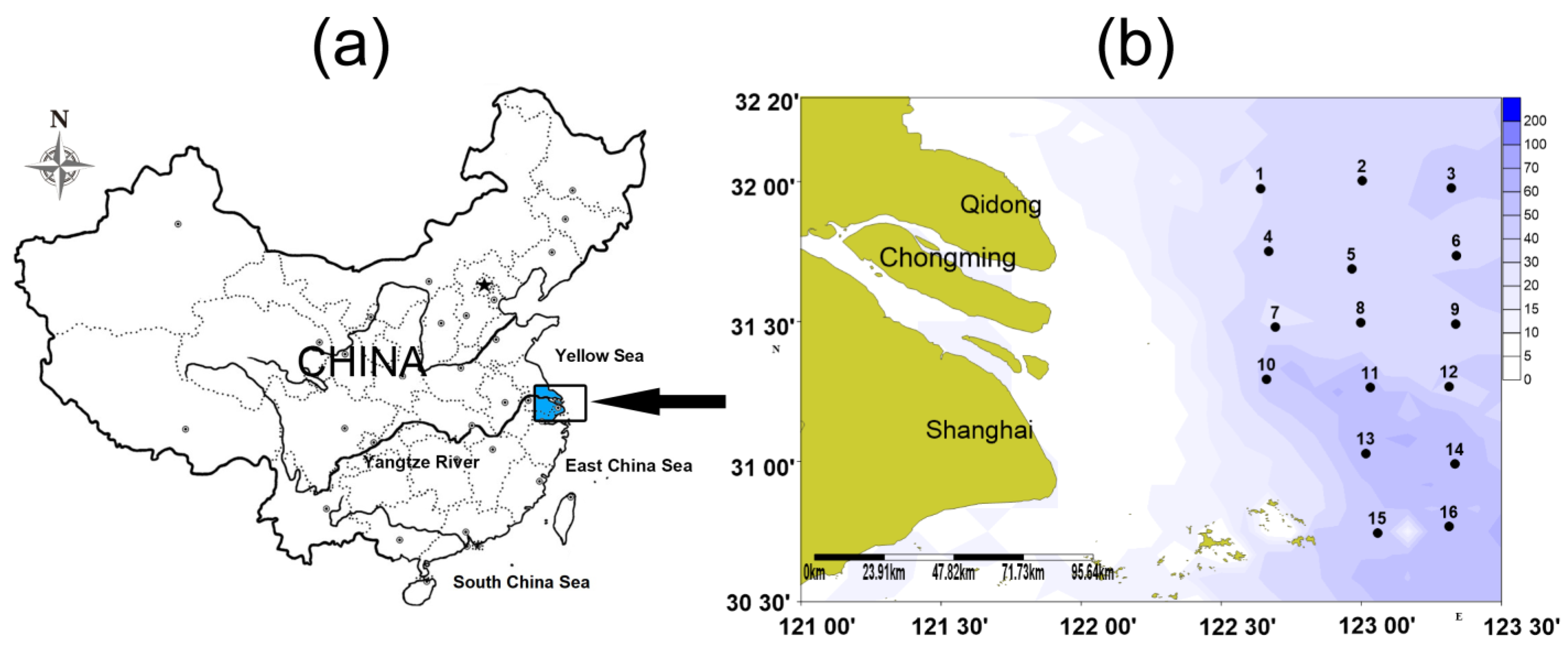
2.1. Sample Collection

Biological and oceanographic data were collected yearly during the fall in fishery evaluation cruises (November 2012, November 2013, November 2014, November 2015 and November 2016). Due to the fishing prohibition policy, water depth requirements, and safety considerations for trawlers, our trawlers could not enter the shallow water (usually with low salinity) within the Yangtze Estuary for trawl sampling (Figure 1). Weather and equipment failure resulted in not all of the sites being sampled for each survey. Sampling was conducted at 14 stations in 2013 and 15 stations in the remaining years.
The survey vessel was a 255 kW bottom double trawler, the survey gear was a 150.5 m × 96.5 m trawl, the perimeter of the net mouth was 150.5 m, the upper line length was 66 m, the lower line length was 73 m, the maximum mesh of the net was 200 mm, the mesh size decreased from the net body to the cod-end, and the cod-end was 30 mm. When measured at sea, the net headline height during trawling was 9–11 m, the average distance between the net sleeves was 18 m, and the trawling speed of each station was 2–3 Kn and the trawling time was 0.5–1 h.
All catches were cryopreserved and sent back to the laboratory for identification and classification. Each fish was measured in length and weighed. Conductivity, temperature, and depth (CTD) equipment recorded salinity (S), temperature (T), and depth (D) at each station. Surface water was collected, cryopreserved, and brought back to the laboratory for analysis (pH, total suspended particles (TSP), dissolved oxygen (DO), chemical oxygen demand (COD), total nitrogen (TN), total phosphorus (TP), and chlorophyll a (Chl a)). Total nitrogen and total phosphorus were measured by a QuAAtro continuous-flow analyzer, total suspended matter was measured by filtration, chemical oxygen demand and dissolved oxygen were measured by iodine titration, and chlorophyll a was measured by fluorescence extraction. All of these were determined in the study in accordance with GB/T 12763–2007, Specifications for Oceanographic Surveys.

2.2. Data Analysis

Species abundance and biomass at each station were expressed as 103 individuals per km2 (103 ind. km−2) and kilogram per km2 (kg km−2), respectively. The dominant fish species were classified using the index of relative importance (IRI), calculated as:
IRI = (N% + W%) × F% × 10,000,
where N% and W% are the relative abundance and biomass, respectively. F% is the percentage frequency of occurrence of the species in all stations.
Only species occurring in at least two stations were included in the follow-up data analysis [19].
When SPSS version 27.0 was used to calculate the significance of interannual differences in the 10 environmental factors (S, D, T, pH, COD, TSP, DO, TN, TP, and Chla), Levene’s and Kolmogorov–Smirnov tests were applied to determine data homoscedasticity and normality, respectively. For environmental data that could not meet both requirements, square root (x1/2) or log transformation (log10(x + 1)) were performed, and for those that could meet both conditions after transformation, one-way ANOVA was performed on the transformed data; for those that still could not meet the requirements, the non-parametric Kruskal–Wallis test was used. The significance of differences in environmental data among years was compared using the paired comparison method.
The spatial distribution of abundance and biomass was visualized by drawing distribution maps using SURFER version 12.0. Annual and spatial variation in fish assemblage structure was analyzed by PRIMER version 6.0 [20,21]. First, fish species with frequencies greater than 5% were used to analyze the assemblage structure and its relationship with environmental factors to reduce the influence of rare species. Based on log10(x + 1) abundance data (to reduce the effect of dominant fish species), the Bray–Curtis similarity matrix was constructed. Non-metric multidimensional scaling (NMDS) was then used to identify annual variation in fish assemblage structure. Non-parametric similarity analysis was performed using ANOSIM to determine the significance of inter-annual and spatial variation in fish assemblage structure. The similarity percentage analyses based on the abundance of fish species were performed with SIMPER to detect typical species contributing most to the similarity in each observed assemblage (cumulative percentage above 90%) and its contribution percentage.
Canoco5.0 was used to study the relationship between environmental variables and fish assemblages (canonical correspondence analysis (CCA) or redundancy analysis (RDA)). Detrended correspondence analysis (DCA) was first performed to determine a suitable response according to the maximum gradient length of the first DCA axis (>4, CCA; >4 and <3, CCA or RDA; <3, RDA) [18]. The maximum gradient length is 2.3 SD, so RDA was chosen. Log (x + 1) conversion of abundance and environment data was carried out to minimize the effects of extreme values and zeros. The Monte Carlo permutation test was used to identify the key factors that significantly affect the fish assemblages (p < 0.05).

3. Results

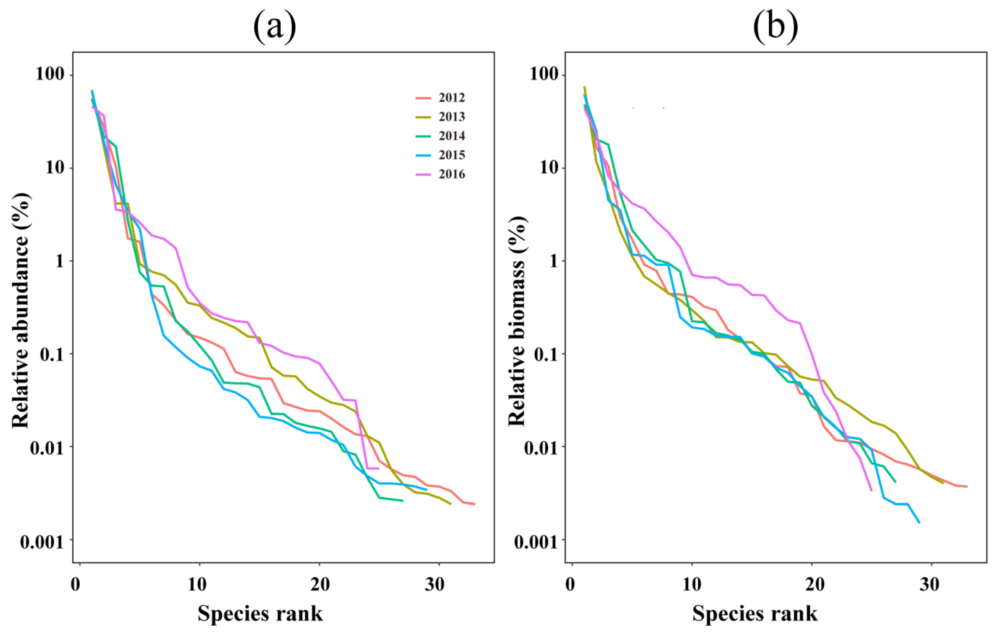
3.1. Faunal Composition

In total, 64 fish species referable to 14 orders and 39 families were identified. Of these, 20 species (31.25%) occur in all years (Figure 2a) and 24 (37.5%) occur in singular years. Aulopiformes, Perciformes, and Clupeiformes account for the highest proportion of the overall fish abundance (Figure 2b). All Aulopiformes captured from the autumns of 2012–2016 were Harpadon nehereus, Perciformes contained 27 fish species, and Clupeiformes contained 10 fish species. The remaining orders account for a very low proportion of fish abundance. The depth range, climate zone/temperature range, and distribution of all fish caught in the offshore waters of the Yangtze Estuary during the autumns of 2012–2016 are listed in Table S1.

3.2. Environment Variables

Of the ten environmental factors examined, nine differ significantly among the years, while no significant difference is detected in depth (Table 1). Station depth varies from 23 m to 62 m. Salinity is significantly higher in 2013 than in 2014–2016, while the temperature is significantly lower in 2012 and 2014 than in the other years. Both dissolved oxygen and pH peak in 2012, with significant inter-annual variation, but with different trends over time. Chemical oxygen demand, on the contrary, has the lowest value in 2012 and significantly lower than in other years. Both total nitrogen and total phosphorus show their lowest values in 2016, with the difference being that total nitrogen peaks in 2014 and total phosphorus peaks in 2015. TSP is significantly lower in 2014 and 2015 than in other years, while chlorophyll a is significantly lower in 2012 and 2014 than in the other years.

3.3. Annual Variation in Fish Assemblages and Relationships with Environmental Factors

Annual variations in fish abundance and biomass are shown in Figure 3a. Abundance is highest in 2013 and gradually decreases, and biomass is highest in 2013 and lowest in 2015, with partial differences between the abundance and biomass trends. Annual variation in fish assemblage structure is portrayed in the NMDS ordination plot, one-way ANOSIM (R-value and significance level), and SIMPER analysis (Figure 3b; Table 2). The year 2015 is significantly different from all other years (p < 0.05). The years with no significant difference on the NMDS plot are close in position or even overlap, and the years with significant differences are clearly distinguished by fish assemblages.
Harpadon nehereus is the most dominant fish species, with the highest IRI values in the five years (Table 3). Trichiurus japonicus is the second dominant species after Harpadon nehereus. These two species are the dominant species in each year from 2012–2016, occupying an absolutely dominant position in the studied area. In 2016, the most dominant species consists of five species, with four dominant species in 2013 and 2014, and three dominant species in 2012 and 2015.
The relative abundance, biomass, and species evenness of fish assemblages from 2012–2016 are reflected by the rank–abundance curves (Figure 4). The longer span on the horizontal axis for the curves in 2012 and 2013 compared to the other years indicates higher species richness. Both the abundance and biomass curves have large gradients with steep descending slopes, indicating low evenness and a large proportion of dominant species in total abundance (96.72%) and total biomass (95.88%).
Based on the Monte Carlo tests of the F-ratios (p < 0.05), total suspended particles, depth, and dissolved oxygen are the most significant environmental variables driving the spatiotemporal variation in fish assemblages. The RDA results relate the annual variation in fish assemblages in the Yangtze Estuary to the environmental descriptors considered, such as total suspended particles, depth, and dissolved oxygen (Figure 5a). Total suspended particles and dissolved oxygen are the main environmental factors driving the interannual variation in fish assemblages. According to the results of the ANOSIM and SIMPER analyses, fish assemblages in 2015 are significantly different from other years, associated with low total suspended particles and low dissolved oxygen. Fish assemblages in 2012 are in high total suspended particles and high dissolved oxygen positions. Fish assemblages in 2013, 2014, and 2016 are associated with moderate total suspended particles and dissolved oxygen.
The location of species on the RDA diagram indicates their habitat preferences on an environmental gradient [22] (Figure 5b). Most fish are in the medium range of dissolved oxygen and total suspended particles, and a few are in the high or low range of dissolved oxygen and total suspended particles. Uranoscopus japonicus, Takifugu obscurus, and Engraulis japonicus are more abundant at sites with lower total suspended particles and dissolved oxygen, whereas Collichthys lucidus, Harpadon nehereus, Coilia nasus, and Setipinna taty are more abundant at sites with higher total suspended particles and dissolved oxygen. The degree of interpretation of the RDA results is shown in Table 4.
Correlations between environmental factors during the autumns of 2012–2016 are demonstrated in Figure 5c, with the strongest positive correlations between temperature and salinity. The correlations between total suspended particles and dissolved oxygen, the main environmental factors driving temporal variation in fish assemblages, are not strong. Unlike Figure 5a, which shows the driving environmental factors that cause interannual variation in fish assemblages, Figure 5c shows the relationship between a particular fish assemblage itself and environmental factors. Among them, depth, dissolved oxygen, and pH are significantly correlated with the annual fish assemblage.

3.4. Spatial Characteristics of the Fish Assemblages

Due to the large environmental gradient in the offshore waters of the Yangtze Estuary, there are significant spatial differences in the abundance, biomass, and assemblage structure of fish assemblages in the autumns of 2012–2016 (Figure S1). Among the environmental factors affecting the structure of fish assemblages, total suspended particles and dissolved oxygen drive the interannual variation of fish assemblages, while depth drives their spatial structure variation. Based on the position of the fish assemblages on the RDA ordination plots (Figure 6a), the fish assemblages are separated into two groups, corresponding to shallow assemblage and deep assemblage, and the corresponding spatial distribution locations are shown in Figure 6c. The ANOSIM analysis reveals significant differences in the shallow and deep assemblage structures (R = 0.103, p = 0.001). The average similarities within the shallow and deep fish assemblages are 43.82% and 32.48%, respectively, while the average dissimilarity between them is 64.89% (indicating that the fish assemblages differ between the areas).
According to the contribution of the different fish species to the two assemblages, the fish species can be divided into deep and shallow typical species (Table 5). The RDA analysis of the two groups of fish and environmental factors shows that most of the typical deep assemblage fish species are mainly located in the bottom-right of the plot, which is positively correlated with depth, and the typical shallow assemblage fish species are mainly located in the top-left of the plot, which shows a negative correlation with depth (Figure 6c). Figure 6d shows the relationship between the deep and shallow fish assemblages themselves and environmental factors. Among them, the shallow fish assemblage is significantly correlated with pH.
Among all environmental variables, the depth and total suspended particles are significantly different between shallow and deep areas, and the total suspended particles are significantly higher in the shallow waters (F = 6.137, p < 0.05) (Table 6). There are no significant differences in the remaining environmental factors between shallow and deep areas.

4. Discussion

4.1. Composition of the Fish Assemblages

In the present study, a total of 64 fish species were caught in the offshore waters of the Yangtze Estuary during the autumns of 2012–2016, which is clearly at a low level compared to the autumns of 2002–2005 [17]. The number of fish species caught in our study also decreases from 41 in 2012 to 29 in 2016. This is closely related to the effects of high-intensity fishing and changes in the offshore marine environment on fish spawning and bait grounds in the last decade [7,23]. The ichthyoplankton assemblage in the Yangtze Estuary has also declined from 94 species in the 1980s to 26 species in 2013–2020, and the replenishment capacity of the fishery resources has decreased substantially [24,25]. Tropical and subtropical estuaries have higher species richness than temperate systems [26]. The number of fish species in the waters of the Pearl River Estuary is much greater than in the waters of the Yangtze River estuary [27]. In Zuari, a well-mixed tropical estuary located along the southwest coast of India, the number of fish species can reach 224 in the same period [28].
Combinations of a large number of rare species and a few highly abundant species are common features of temperate estuarine faunae [29,30]. Due to the mixed water masses in the Yangtze Estuary, not all of the species are adapted to the local conditions [31]. The sensu stricto freshwater and marine species do not occur in the offshore waters of the Yangtze Estuary or occur in small numbers at very few stations for only a short period of time. For example, the Yangtze River’s abundant freshwater fish such as Mylopharyngodon piceus and Ctenopharyngodon idella do not appear in the offshore waters of the Yangtze Estuary, while Johnius distinctus, which is a marine fish, only occurs in two stations in 2015 [32]. In the present study, only six of the species caught in the Yangtze Estuary dominate with IRI values > 500. The dominant species account for a significant proportion of total abundance (96.72%) and total biomass (95.88%), and species homogeneity is low. In comparison with the autumn fish in the Yangtze River estuary from 2002 to 2005, the dominant species do not differ much, but the dominance of the traditionally dominant species decreases, and the species with absolute dominance changes from Trichiurus japonicus to Harpadon nehereus [17]. The structure of fishery resources in the Yangtze Estuary has changed significantly, with the decline in traditional fishery resources and the miniaturization of fish [33]. This phenomenon is manifested in the offshore waters of the Yangtze Estuary by the decline in traditional large economic species resources and the gradual dominance of small secondary economic species fish [34]. The protection and restoration of fishery resources urgently need to be strengthened.

4.2. Annual Variation in Fish Assemblages

Estuaries are highly dynamic ecosystems with complex physical, chemical, and hydrological conditions that change dramatically over time [26,35,36]. In this study, all environmental factors except depth exhibit significant interannual differences, which further influences the abundance, biomass, and composition structure of the fish communities. In the autumns of 2002–2005, water temperature and salinity were the main environmental factors causing the interannual variation of fish in the Yangtze Estuary [17]. In the spring of 2004 and 2007, the temperature was still the main environmental factor driving fish community variation in the Yangtze Estuary [1]. In addition to the Yangtze Estuary, in a small macrotidal estuary (the Canche, France), temperature, salinity, and Crangon crangon (a potential predator for young-of-the-year fish or prey for older ones) were the three most important factors influencing fish species richness and abundance [37]. Temperature and salinity have relatively strong effects on the temporal variation of most estuarine fish, but there are exceptions. In a sample survey of the subtidal fish assemblage of the Tagus estuary coastal area, depth and sediment type were the main structural factors in the fish assemblage. Temperature and salinity were less important to the overall assemblage structure, although this may be due to the particular climatic regime of the sampling year [38]. In this survey, due to the fixed sampling season, temperature and salinity show little difference in the autumn and do not become the main influencing factors. Total suspended particles and dissolved oxygen are the main environmental driving factors for the temporal variation of fish assemblage structure in the offshore waters of the Yangtze Estuary during the autumns of 2012–2016, and the correlation between them is not strong.
During the spring and fall of 1998–2001 and the autumn of 2001, there was no significant intervention effect of total suspended particles on the variations in fish assemblages [15,39]. In this study, total suspended particles are the dominant environmental factor driving fish assemblages in the Yangtze Estuary in the autumn. Total suspended particle concentrations are mainly influenced by benthic sediment resuspension, riverine inputs, upwelling, and plankton [40,41]. Wind direction also plays a significant role in the dispersal of total suspended particle concentrations, with southerly winds favoring the dispersal of high total suspended particle concentrations offshore and easterly winds inhibiting expansion [42]. In 2012–2016, the cumulative effect of Yangtze River input and the diffusion effect of higher wind speeds and southerly winds resulted in the highest level of total suspended particles in 2013 [42]. There was a good log–linear relationship between the total suspended matter concentration and turbidity in the offshore waters of the Yangtze Estuary, and the influencing mechanism on fish distribution was consistent [43]. High turbidity increases the survival rate of estuarine fish by keeping juveniles and small adults away from visual predators and providing more available food [44]. There are many small fish in the turbidity waters, which are an important food for marine carnivorous fish. Carnivorous fish may choose their habitat based on a balance of factors such as the consumption and time of predation in turbidity waters [45]. The changing trend of fish biomass in the autumns of 2012–2016 is basically consistent with the change in total suspended particles, that is, the higher the concentration of total suspended matter, the higher the fish biomass, which is consistent with the above results. In terms of fish assemblage structure, RDA shows that fish such as Harpadon nehereus and Collichthys lucidus are associated with high total suspended matter concentrations. Harpadon nehereus show stronger feeding in the autumn, with the highest stomach fullness coefficient, and, therefore, prefer areas with higher bait organisms [10,31]. In the present study, high total suspended matter concentrations in the Yangtze Estuary in the autumn of 2013 provide more feeding opportunities for Harpadon nehereus, and, thus, their abundance and biomass reach their highest values in 2013.
Dissolved oxygen is another main factor driving the interannual variation of fish aggregation in the Yangtze Estuary from 2012 to 2016. Dissolved oxygen content in seawater is an important reference item to determine the biological growth level and seawater pollution level in the sea area [46]. Dissolved oxygen, as a basic condition for the survival of aquatic animals, is an important environmental factor affecting the growth, respiration, material, and energy metabolism of aquatic animals [47]. When the dissolved oxygen concentrations drop to 5.0 mg/L, some fish experience respiratory distress, and when dissolved oxygen levels fall below 2.0 mg/L or below 3.0 mg/L, low-dissolved-oxygen sea zones can form [48]. The hypoxic zone in the Yangtze Estuary is mostly formed in the summer, and the hypoxic phenomenon soon subsides after September, and dissolved oxygen content increases, so there is no hypoxic zone in the autumn [49]. Hajisamae et al. found a significant positive correlation between dissolved oxygen in the water and fish biomass [50]. Keller et al. reported a significant decrease in biomass and species diversity of benthic organisms along a low oxygen gradient [51]. Hypoxia may also reduce growth, reproductive success, and recruitment success [52]. In this study, dissolved oxygen reaches its highest value in 2012 and its lowest value in 2015, with significant differences. There is no positive correlation between dissolved oxygen and fish biomass, which may be influenced by the synergistic effect of other environmental factors and human activities. The different preferences and adaptability of different fish species to dissolved oxygen also affect the species composition of fish in the different years [53,54,55]. The RDA shows that fish such as Benthosema pterotum, Vespicula trachinoides, Decapterus maruadsi, and Lateolabrax japonicus are associated with high dissolved oxygen levels. Benthosema pterotum and Decapterus maruadsi, as pelagic fish, require higher dissolved oxygen content [10,56]. Lateolabrax japonicus is sensitive to dissolved oxygen, and low oxygen stress can cause significant oxidative damage to the juvenile Lateolabrax japonicus organism; therefore, Lateolabrax japonicus prefers areas of high dissolved oxygen, which in the Yangtze Estuary only occurred in 2012 when dissolved oxygen was high [57].
In addition to environmental changes, high-intensity fishing is also an important reason for the interannual variation of fish assemblages. With the increase in fishing efforts, fishing intensity far exceeds resource replenishment capacity, and major economic fish in the Yangtze River estuary are now overfished [10]. In this study, fish total abundance decreases year by year after reaching its peak in 2013, and it reaches its lowest value in 2016, which is only 19.25% of the abundance in 2013. Therefore, it is imperative to protect the ecological environment of the Yangtze Estuary, limit the fishing intensity, and standardize the use of fishing gear.

4.3. Spatial Characteristics of the Fish Assemblages

Coastal areas are important habitats for many marine fish, and there are often large gradients in environmental conditions that result in different species assemblages [58]. Depth is an important variable in estuarine ecosystems and is closely related to the distribution of marine organisms, light intensity, food availability, and temperature [59]. In this study, the range of depths in the Yangtze Estuary is 23–62 m, with large spatial variation driving spatial variation in fish assemblages, but no significant interannual variation in time. This spatial variability is largely a product of the different spatial patterns exhibited by different species [60]. The fish are classified into shallow assemblage and deep assemblage according to depth. The species have their own preferences for the water layers, with 19 species preferring to live in the deeper areas, 13 species preferring shallow areas, and deep assemblage having a higher species diversity.
Depth has historically been an important factor, but it is not the only factor driving spatial variability in the Yangtze Estuary. In this study, total suspended matter also differs significantly in the deep areas and shallow areas, suggesting that total suspended matter drives interannual variation along with spatial variation in fish assemblages. Total suspended matter concentrations are lower in the deep area near the outer sea and higher in the shallow area near the estuary. In 2004 and 2007, depth, salinity, and total suspended matter together drove variation in the spatial structure of spring fish assemblages in the Yangtze Estuary, dividing fish into southern and northern assemblages [1]. The invertebrate assemblage in the Yangtze Estuary was also divided into shallow assemblage and deep assemblage according to depth [61]. In addition to depth, the spatial variation in fish assemblages in the Yangtze Estuary is also driven by other environmental factors at different times. In 2018, the spatial variation in fish in the Yangtze Estuary was driven by salinity, which was divided into high-salt assemblage and low-salt assemblage depending on salinity [18]. With the exception of the Yangtze Estuary, significant spatial variability is an essential feature of most estuaries (except those with high mixing uniformity) [28,62,63]. On the Alaska Beaufort Shelf, significant interactions between depth and along-shelf position helped define six geographic regions [64]. Continuously changing environmental gradients underlie the spatial variability in estuarine fish communities.
Biotic interactions and human activities may act in conjunction with environmental preferences in the spatial selection of fish. Fish select their preference for environmental conditions while also integrating the effects of solicitations, interspecific competition, predator avoidance, and human activities [58]. Flow alterations caused by dam construction, pollution, habitat destruction, and other human activities can all lead to variations in fish biomass and community structure. Therefore, further studies should quantify the importance of biological effects and human activities on the spatial and temporal distribution of fish to generate more reliable assessments of fish assemblage dynamics and facilitate our development of more rational and effective fisheries conservation strategies.

5. Conclusions

We reported on the spatial and temporal variability in fish assemblages in the Yangtze Estuary over five years in the autumn and their relationships with environmental factors. The fish assemblage in the offshore waters of the Yangtze Estuary is characterized by a few highly abundant species and many rare species. The spatial and temporal variability in fish assemblages is significant. Total suspended particles and dissolved oxygen drive interannual variation in fish abundance, biomass, and species composition, and depth drives spatial variation in the fish. Depending on the depth, the fish were classified and divided into shallow assemblage and deep assemblage. It is worth noting that interactions between fish organisms and human activities may also influence species distribution and could be considered further in future studies.

Supplementary Materials

The following supporting information can be downloaded at: https://www.mdpi.com/article/10.3390/d15050669/s1, Figure S1: Temporal and spatial variation of fish abundance and biomass in the adjacent waters of the Yangtze Estuary during autumn of 2012–2016; Table S1: The depth range, climate zone/temperature range, and distribution of all fish caught in the offshore waters of the Yangtze Estuary during the autumns of 2012–2016.

Author Contributions

Z.C. analyzed the data and completed the first draft. W.X. provide guidance on the structure of the paper. C.L. made suggestions on this paper. All authors made modifications to this paper. All authors participated in revising the manuscript. All authors have read and agreed to the published version of the manuscript.

Funding

This work is financially supported by the National Key R&D Program of China (2022YFF0802202); National Natural Science Foundation of China (No. 31872568); Chinese Academy of Sciences Network Security and Informatization Special Application Demonstration Project (CAS-WX2021SF-0108); The Comprehensive Safety Monitoring System of Three Gorges Project, Reservoir Operation and Management Fund (No. 2136703).

Institutional Review Board Statement

Not applicable.

Data Availability Statement

Not applicable.

Acknowledgments

We thank the scientists and crew of the “Zhe Shengyu 10201” for sampling assistance. We are grateful to the editors and reviewers for their constructive feedback concerning our work.

Conflicts of Interest

The authors state that the research was conducted without any commercial or financial relationship that could be considered as potential conflict of interest.

References

  1. Zhang, Y.Q.; Xian, W.W.; Li, W.L. Fish Assemblage Structure in Adjacent Sea of Changjiang Estuary in Spring of 2004 and 2007 and Its Association with Environmental Factors. Period. Ocean Univ. China 2013, 43, 67–74. [Google Scholar]
  2. Elliott, M. The forth estuary: A nursery and overwintering area for North Sea fishes. Hydrobiologia 1990, 195, 89–103. [Google Scholar] [CrossRef]
  3. Wasserman, R.J.; Strydom, N.A. The importance of estuary head waters as nursery areas for young estuary– and marine–spawned fishes in temperate South Africa. Estuar. Coast. Shelf Sci. 2011, 94, 56–67. [Google Scholar] [CrossRef]
  4. Sheaves, M.; Johnston, R.; Connolly, R.M.; Baker, R. Importance of estuarine mangroves to juvenile banana prawns. Estuar. Coast. Shelf Sci. 2012, 114, 208–219. [Google Scholar] [CrossRef]
  5. Shao, H.B. Research on Composition, Distribution and Influencing Factors of Suspended Matters in the Yangtze River Estuary in Fall. Master’s Thesis, Ocean University of China, Qingdao, China, 2012. [Google Scholar]
  6. Luo, B.Z.; Shen, H.T. The Three Gorges Project and the Ecological Environment of Yangtze Estuary; Science Press: Beijing, China, 1994; pp. 1–32. [Google Scholar]
  7. Xin, M. Long–Term Variations of the Key Environmental Factors and Their Ecological Effects in the Changjiang Estuary. Ph.D. Thesis, Ocean University of China, Qingdao, China, 2014. [Google Scholar]
  8. Vaquer-Sunyer, R.; Duarte, C.M. Thresholds of hypoxia for marine biodiversity. Proc. Natl. Acad. Sci. USA 2008, 105, 15452–15457. [Google Scholar] [CrossRef]
  9. Meier, H.E.M.; Eilola, K.; Almroth-Rosell, E.; Schimanke, S.; Kniebusch, M.; Hoglund, A.; Pemberton, P.; Liu, Y.; Vali, G.; Saraiva, S. Disentangling the impact of nutrient load and climate changes on Baltic Sea hypoxia and eutrophication since 1850. Clim. Dynam. 2019, 53, 1145–1166. [Google Scholar] [CrossRef]
  10. Zhuang, P. Fishes of the Yangtze Estuary; China Agriculture Press: Beijing, China, 2018. [Google Scholar]
  11. Shen, X.Q.; Shi, Y.R.; Chao, M.; Quan, W.M.; Huang, H.J.; Wu, Q.Y. Analysis of taxonomic diversity of fish community in Yangtze River estuary. Prog. Mater. Sci. 2013, 34, 1–7. [Google Scholar]
  12. Wu, J.H.; Wang, J.Q.; Dai, X.J.; Tian, S.Q.; Liu, J.; Chen, J.H.; Wang, X.F. An analysis of spatial co–occurrence pattern of fish species of Yangtze River estuary based on probabilistic model. South China Fish. Sci. 2019, 15, 1–9. [Google Scholar]
  13. Wang, Y.C.; Liang, C.; Xian, W.W.; Wang, Y.B. Using the LBB Method for the Assessments of Seven Fish Stocks From the Yangtze Estuary and Its Adjacent Waters. Front. Mar. Sci. 2021, 8, 679299. [Google Scholar] [CrossRef]
  14. Liu, S.H.; Yang, Y.Y.; He, Y.L.; Ji, X.; Wang, Y.T.; Zhang, H.J.; Mao, R.Y.; Jiang, X.S.; Cheng, X.S. Morphological classification of ichthyoplankton in the Changjiang River Estuary based on DNA barcoding. Acta. Oceanol. Sin. 2021, 43, 93–104. [Google Scholar]
  15. Yu, H.C.; Xian, W.W. The environment effect on fish assemblage structure in waters adjacent to the Changjiang (Yangtze) River estuary (1998–2001). Chin. J. Oceanol. Limnol. 2009, 327, 443–456. [Google Scholar] [CrossRef]
  16. Zhang, H.; Xian, W.W.; Liu, S.D. Ichthyoplankton assemblage structure of springs in the Yangtze Estuary revealed by biological and environmental visions. PeerJ 2015, 3, e1186. [Google Scholar] [CrossRef]
  17. Li, J.S.; Li, S.F.; Cheng, J.H. Analysis on the annual variations of fish resources in the offshore water of Yangtze Estuary in autumn. Mar. Fish. 2008, 2, 120–125. [Google Scholar]
  18. Chen, Z.M.; Ren, Q.Q.; Liu, C.L.; Xian, W.W. Seasonal and Spatial Variations in Fish Assemblage in the Yangtze Estuary and Adjacent Waters and Their Relationship with Environmental Factors. J. Mar. Sci. Eng. 2022, 10, 1679. [Google Scholar] [CrossRef]
  19. Almeida, C.; Coelho, R.; Silva, M.; Bentes, L.; Monteiro, P.; Ribeiro, J.; Erzini, K.; Goncalves, J.M.S. Use of different intertidal habitats by faunal communities in a temperate coastal lagoon. Estuar. Coast. Shelf Sci. 2008, 80, 357–364. [Google Scholar] [CrossRef]
  20. Clarke, K.; Warwick, R. Similarity-Based testing for community pattern—The 2-way layout with no replication. Mar. Biol. 1994, 118, 167–176. [Google Scholar] [CrossRef]
  21. Clarke, K.R. Non-parametric multivariate analyses of changes in community structure. Aust. J. Ecol. 1993, 18, 117–143. [Google Scholar] [CrossRef]
  22. Chu, C.; Jones, N.E. Spatial variability of thermal regimes and other environmental determinants of stream fish communities in the Great Lakes Basin, Ontario, Canada. River Res. Appl. 2011, 27, 646–662. [Google Scholar] [CrossRef]
  23. Chen, Y.L. Spatio–Temporal Variation of Fishery Resources in the Yellow Sea and Yangtze River Estuary. Ph.D. Thesis, Institute of Oceanography, Chinese Academy of Sciences, Qingdao, China, 2017. [Google Scholar]
  24. Yang, D.; Wu, G.; Sun, J. The investigation ok pelagic eggs, larvae and juveniles of fishes at the mouth of the Changjiang river and adjacent areas. Oceanol. Limnol. Sin. 1990, 4, 346–355. [Google Scholar]
  25. Wang, Y.B.; Liang, C.; Chen, Z.M.; Liu, S.D.; Zhang, H.; Xian, W.W. Spring Ichthyoplankton Assemblage Structure in the Yangtze Estuary Under Environmental Factors. Front. Mar. Sci. 2021, 8, 806096. [Google Scholar] [CrossRef]
  26. Whitfield, A.K. Fish species diversity in Southern African estuarine systems: An evolutionary perspective. Environ. Biol. Fishes 1994, 40, 37–48. [Google Scholar] [CrossRef]
  27. Zheng, L.; Zhen, B.; Li, F.; Xu, B.Q.; Li, M.; Yang, F.Z. Comparison of ontaxonomic diversity of fish community among the Yellow River estuary, Yangtze River estuary, Pearl River estuary and their adjacent waters. J. Dalian Ocean Univ. 2014, 29, 530–535. [Google Scholar]
  28. Sreekanth, G.B.; Jaiswar, A.K.; Zacharia, P.U.; Pazhayamadom, D.G.; Chakraborty, S.K. Effect of environment on spatio–temporal structuring of fish assemblages in a monsoon–influenced tropical estuary. Environ. Monit. Assess. 2019, 191, 305. [Google Scholar] [CrossRef] [PubMed]
  29. Drake, P.; Arias, A.M.; Baldó, F.; Cuesta, J.A.; Rodríguez, A.; Silva–Garcia, A.; Sobrino, I.; García–González, D.; Fernández–Delgado, C. Spatial and temporal variation of the nekton and hyperbenthos from a temperate European estuary with regulated freshwater inflow. Estuaries 2002, 25, 451. [Google Scholar] [CrossRef]
  30. Jackson, G.; Jones, G. Spatial and temporal variation in nearshore fish and macroinvertebrate assemblages from a temperate Australian estuary over a decade. Mar. Ecol. Prog. Ser. 1999, 182, 253–268. [Google Scholar] [CrossRef]
  31. Luo, B.Z. Ecological characteristics and fishery resources of the Yangtze River Estuary and adjacent sea. Resour. Environ. Yangtze Val. 1992, 1, 24–30. [Google Scholar]
  32. Li, H.J. Effects of Broodstock Enhancement on Fish Larval Resources and Genetic Diversity of the Four Major Chinese Carps in the Middle Reaches of the Yangtze River. Master’s Thesis, Southwest University, Chongqing, China, 2019. [Google Scholar]
  33. Luo, H.Z. Study of Main Biology Character and Analysis of Resource Status on the Harpadon nehereus. Master’s Thesis, Zhejiang Ocean University, Zhoushan, China, 2012. [Google Scholar]
  34. Du, X.X. Biological Characteristics and Spatial Distribution Patter of Harpadon nehereus in Offshore Water of Southern Zhejiang. Master’s Thesis, Shanghai Ocean University, Shanghai, China, 2018. [Google Scholar]
  35. Flint, R.W. Long–term estuarine variability and associated biological response. Estuaries 1985, 8, 158–169. [Google Scholar] [CrossRef]
  36. Harris, S.A.; Cyrus, D.P. Occurrence of fish larvae in the St Lucia Estuary, Kwazulu–Natal, South Africa. S. Afr. J. Mar. Sci. 1995, 16, 333–350. [Google Scholar] [CrossRef]
  37. Selleslagh, J.; Amara, R. Environmental factors structuring fish composition and assemblages in a small macrotidal estuary (eastern English Channel). Estuar. Coast. Shelf Sci. 2008, 79, 507–517. [Google Scholar] [CrossRef]
  38. Prista, N.; Vasconcelos, R.P.; Costa, M.J.; Cabral, H. The demersal fish assemblage of the coastal area adjacent to the Tagus estuary (Portugal): Relationships with environmental conditions. Oceanol. Acta 2003, 26, 525–536. [Google Scholar] [CrossRef]
  39. Zhang, Y.Q. Environmental Impact on the Fish Assemblage Structure in Adjacent Sea Area of the Yangtze River Estuary. Master’s Thesis, Institute of Oceanography, Chinese Academy of Sciences, Qingdao, China, 2012. [Google Scholar]
  40. Suzumura, M.; Kokubun, H.; Arata, N. Distribution and characteristics of suspended particulate matter in a heavily eutrophic estuary, Tokyo Bay, Japan. Mar. Pollut. Bull. 2004, 49, 496–503. [Google Scholar] [CrossRef]
  41. Qin, Y.S.; Li, F.; Xu, S.M.; Milliman, J.; Limeburner, R. Suspended matter in the south yellow sea. Oceanol. Limnol. Sin. 1989, 20, 101–112. [Google Scholar]
  42. Xue, W.J.; Qiao, L.L.; Zhong, Y.; Xue, C.; Chen, S.G.; Li, S.H.; Liu, P.; Gao, F. Multiple timescale variation in concentration of surface suspended sediment in Changjiang river estuary. Oceanol. Limnol. Sin. 2019, 50, 1002–1013. [Google Scholar]
  43. Zhai, S.K.; Zhang, H.J.; Fan, D.J.; Yang, R.M.; Cao, L.H. Corresponding relationship between suspended matter concentration and turbidity on Changjiang Estuary and adjacent sea area. Acta. Sci. Circumst. 2005, 25, 693–699. [Google Scholar]
  44. Whitfield, A.K. Ichthyofaunal assemblages in estuaries: A South African case study. Rev. Fish Biol. Fish 1999, 91, 51–86. [Google Scholar]
  45. Akin, S.; Buhan, E.; Winemiller, K.O.; Yimaz, H. Fish assemblage structure of Koycegiz Lagoon-Estuary, Turkey: Spatial and temporal distribution patterns in relation to environmental variation. Estuar. Coast Shelf Sci. 2005, 64, 671–684. [Google Scholar] [CrossRef]
  46. Zhang, Y.Y.; Zhang, J.; Wu, Y.; Zhu, Z.Y. Characteristics of Dissolved Oxygen and Its Affecting Factors in the Yangtze Estuary. J. Environ. Sci. 2007, 28, 1649–1654. [Google Scholar]
  47. Wu, R.S. Hypoxia: From molecular responses to ecosystem responses. Mar. Pollut. Bull. 2002, 45, 35–45. [Google Scholar] [CrossRef]
  48. Diaz, R.J.; Rosenberg, R. Spreading dead zones and consequences for marine ecosystems. Science 2008, 321, 926–929. [Google Scholar] [CrossRef]
  49. Wang, P.H.; Li, B. Historical Changes and Mechanism of Hypoxia in the Changjiang Estuary and Its Adjacent Waters. J. Zhejiang Ocean. Univ. 2019, 38, 401–406. [Google Scholar]
  50. Hajisamae, S.; Yeesin, P. Patterns in community structure of trawl catches along coastal area of the south China sea. Raffles Bull. Zool. 2010, 58, 357–368. [Google Scholar]
  51. Keller, A.A.; Simon, V.; Chan, F.; Wakefield, W.W.; Clarke, M.E.; Barth, J.A.; Kamikawa, D.; Fruh, E.L. Demersal fish and invertebrate biomass in relation to an offshore hypoxic zone along the US west coast. Fish. Oceanogr. 2010, 19, 76–87. [Google Scholar] [CrossRef]
  52. Hassell, K.L.; Coutin, P.C.; Nugegoda, D. Hypoxia impairs embryo development and survival in black bream (Acanthopagrus butcheri). Mar. Pollut. Bull. 2008, 57, 302–306. [Google Scholar] [CrossRef] [PubMed]
  53. Zhu, W.B.; Cui, G.C.; Hu, C.L.; Zhu, H.C.; Wang, Y.L.; Jiang, R.J.; Zhang, Y.Z.; Feng, C.L. Effects of environmental factors on growth and distribution of young chub mackerel scomber japonicus along the coast of zhejiang in spring. Oceanol. Limnol. Sin. 2021, 52, 1448–1455. [Google Scholar]
  54. Liu, X.J.; Huang, G.Q.; Li, J.; Tang, X. Response of Oxidative Stress Indicators in Liver and Muscle of Mullet Liza haematocheila to Variation in Dissolyed Oxygen Levels. Fish. Sci. 2014, 33, 344–349. [Google Scholar]
  55. Wilding, J.L. The oxygen threshold for three species of fish. Ecology 1939, 20, 253–263. [Google Scholar] [CrossRef]
  56. Sun, Y.; Lv, F.H.; Chen, Z.; Diao, X.Y.; Jiang, J.G.; Wei, C.J.; Pan, J. Spatial–temporal distribution and dynamics of dissolved oxygen in an adjacent area of the Changjiang estuary. Mar. Sci. 2021, 45, 86–96. [Google Scholar]
  57. Chang, Z.C.; Wen, H.S.; Zhang, M.Z.; Li, J.F.; Li, Y.; Zhang, K.Q.; Wang, W.; Liu, Y.; Tian, Y.; Wang, X.L. Effects of dissolved oxygen levels on oxidative stress response and energy utilization of juvenile Chinese seabass (Lateolabrax maculatus) and associate physiological mechanisms. Period. Ocean Univ. China 2018, 48, 20–28. [Google Scholar]
  58. Hamilton, B.R.; Peterson, C.T.; Dawdy, A.; Grubbs, R.D. Environmental correlates of elasmobranch and large fish distribution in a river–dominated estuary. Mar. Ecol. Prog. Ser. 2022, 688, 83–98. [Google Scholar] [CrossRef]
  59. Murillo, F.J.; Serrano, A.; Kenchington, E.; Mora, J. Epibenthic assemblages of the Tail of the Grand Bank and Flemish Cap (northwest Atlantic) in relation to environmental parameters and trawling intensity. Deep Sea Res. Part I 2016, 109, 99–122. [Google Scholar] [CrossRef]
  60. Beaudreau, A.H.; Bergstrom, C.A.; Whitney, E.J.; Duncan, D.H.; Lundstrom, N.C. Seasonal and interannual variation in high latitude estuarine fish community structure along a glacial to non–glacial watershed gradient in Southeast Alaska. Environ. Biol. Fishes 2022, 105, 431–452. [Google Scholar] [CrossRef]
  61. Ren, Q.Q.; Xian, W.W.; Liu, C.L.; Li, W.L. Spring–time nektonic invertebrate assemblages of and adjacent to the Yangtze Estuary. Estuar. Coast. Shelf Sci. 2019, 227, 106338. [Google Scholar] [CrossRef]
  62. Chapman, E.D.; Miller, E.A.; Singer, G.P.; Hearn, A.R.; Thomas, M.J.; Brostoff, W.N.; LaCivita, P.E.; Klimley, A.P. Spatiotemporal occurrence of green sturgeon at dredging and placement sites in the San Francisco estuary. Environ. Biol. Fishes 2019, 102, 27–40. [Google Scholar] [CrossRef]
  63. Sheaves, M.; Johnston, R. Ecological drivers of spatial variability among fish fauna of 21 tropical Australian estuaries. Mar. Ecol. Prog. Ser. 2009, 385, 245–260. [Google Scholar] [CrossRef]
  64. Ravelo, A.M.; Konar, B.; Bluhm, B.A. Spatial variability of epibenthic communities on the Alaska Beaufort Shelf. Polar Biol. 2015, 38, 1783–1804. [Google Scholar] [CrossRef]
Figure 1. (a): the geographical location of the Yangtze Estuary; (b): sampling stations in the offshore waters of the Yangtze Estuary during the autumns of 2012–2016, the numbers and dots in the figure represent the different stations (2012: missing station 10; 2013: missing stations 7 and 10; 2014: missing station 7; 2015: missing station 1; 2016: missing station 10). The background color indicates the depth variation.
Diversity 15 00669 g001
Figure 2. Species richness (a) and relative abundance of taxa (b) in the offshore waters of the Yangtze Estuary during the autumns of 2012–2016. (a): in the Venn plot, different colors indicate fish assemblages in different years, and numbers indicate the number of species that are unique or common in a year; UpSet plot showing the fish composition from 2012 to 2016 (e.g., 9 species were found only in 2012 (left), whereas 20 species occurred in the 5 different years).
Diversity 15 00669 g002
Figure 3. Annual variation in fish mean abundance and mean biomass (a), where error bars indicate standard deviations, and the NMDS plot of the fish assemblage structure (b) in the offshore waters of the Yangtze Estuary during the autumns of 2012–2016.
Diversity 15 00669 g003
Figure 4. The relative abundance (a) and biomass (b) of the fish in the offshore waters of the Yangtze Estuary during the autumns of 2012–2016 are reflected in the curve length on the horizontal axes and the evenness of the curve shape.
Diversity 15 00669 g004
Figure 5. RDA plots of fish assemblages (a) and species (b) associated with environmental variables and correlations between fish assemblages and environmental factors (c) in the offshore waters of the Yangtze Estuary during the autumns of 2012–2016, *, **, *** indicates different degrees of correlations. Colu: Collichthys lucidus; Lapo: Larimichthys polyactis; Sppi: Sphyraena pinguis; Scni: Scomberomorus niphonius; Trja: Trichiurus japonicus; Seta: Setipinna taty; Chku: Chelidonichthys kumu; Paar: Pampus argenteus; Hane: Harpadon nehereus; Cona: Coilia nasus; Liha: Liza haematocheila; Laja: Lateolabrax japonicus; Mimo: Minous monodactylus; Sazu: Sardinella zunas; Jobe: Johnius belangerii; Muci: Muraenesox cinereus; Dema: Decapterus maruadsi; Tafl: Takifugu flavidus; Cyse: Cynoglossus semilaevis; Psan: Psenopsis anomala; Comy: Coilia mystus; Thka: Thryssa kammalensis; Anhi: Antennarius hispidus; Taxa: Takifugu xanthopterus; Apli: Apogonichthys lineatus; Enja: Engraulis japonicus; Ilel: Ilisha elongata; Amhe: Chaeturichthys hexanema; Gipu: Girella punctata; Urja: Uranoscopus aponicus; Pear: Pennahia argentata; Hepr: Hemisalanx prognathus; Plco: Pleuronichthys cornutus; Mimi: Miichthys miiuy; Stco: Stolephorus commersonii; Bept: Benthosema pterotum; Scja: Scomber japonicus; Vetr: Vespicula trachinoides; Seru: Secutor ruconius; Cyma: Cynoglossus macrolepidotus; Taob: Takifugu obscurus; Odru: Odontamblyopus ubicundus; Nial: Nibea albiflora. The environment factor code is shown in Table 1.
Diversity 15 00669 g005
Figure 6. RDA ordination plots depicting correlations between fish assemblages (a), fish species (b), and key environmental factors, and the distribution of different assemblages (c) and the correlations between the fish assemblages and environmental factors (d) in the offshore waters of the Yangtze Estuary during the autumns of 2012–2016, *, **, *** indicates different degrees of correlations.
Diversity 15 00669 g006
Table 1. Temporal variation in environmental factors in the offshore waters of the Yangtze Estuary during the autumns of 2012–2016 (Mean ± SD).
Environmental Factors20122013201420152016
Depth (D)42.6 ± 11.1241.14 ± 11.9338.47 ± 8.4137.67 ± 8.0540.4 ± 9.53
Salinity (S)32.3 ± 0.57 bc33.51 ± 0.48 a30.36 ± 2.32 c31.01 ± 3.12 b32.56 ± 1.12 b
Temperature (T) 19.58 ± 0.56 c21.36 ± 0.34 a20.6 ± 0.51 b21.32 ± 0.97 a21.56 ± 0.86 a
Dissolved oxygen (DO)7.4 ± 0.41 a7.26 ± 0.17 ab7.37 ± 1.14 b6.41 ± 0.74 b7.13 ± 0.55 b
pH8.46 ± 0.09 a8.23 ± 0.05 b7.99 ± 0.29 bc7.93 ± 0.05 c8.36 ± 0.13 a
Chemical oxygen demand (COD)0.63 ± 0.31 b0.93 ± 0.26 a1.22 ± 0.82 a1.38 ± 0.83 a1.12 ± 0.38 a
Total nitrogen (TN)13.22 ± 4.5 b16.52 ± 9.16 b28.45 ± 15.05 a19.17 ± 11.48 ab8.37 ± 10.21 c
Total phosphorus (TP)0.69 ± 0.2 cd0.9 ± 0.45 bc0.95 ± 0.21 ab1.13 ± 0.31 a0.6 ± 0.28 d
Total suspended particles (TSP)7.28 ± 5.18 a13.53 ± 17 a2.66 ± 0.85 b2.05 ± 1.53 b5.21 ± 2.15 a
Chlorophyll a (Chl a)0.2 ± 0.04 b0.52 ± 0.15 a0.32 ± 0.5 b0.55 ± 0.41 a0.37 ± 0.16 a
Values with different letters (a–d) indicate significant differences among the years; values with the same characters indicate insignificant differences.
Table 2. Temporal variation in environmental factors in the offshore waters of the Yangtze Estuary during the autumns of 2012–2016 (mean ± SD).
Groups ANOSIMSIMPER
RPAverage Dissimilarity
2012 vs. 20130.0730.05754.32
2012 vs. 2014−0.0050.45754.64
2012 vs. 20150.1880.00676.42
2012 vs. 20160.0950.0462.34
2013 vs. 20140.1490.0151.64
2013 vs. 20150.4330.00177.9
2013 vs. 20160.3740.00162.67
2014 vs. 20150.280.00173.68
2014 vs. 20160.0550.09756.15
2015 vs. 20160.1640.00572.66
Table 3. The dominant fish species in the offshore waters of the Yangtze Estuary during the autumns of 2012–2016. The dominant species in each year are marked in bold.
IRI
Dominant Species20122013201420152016
Collichthys lucidus253.12 533.08337.46 1.08 327.92
Larimichthys polyactis391.90 88.95 289.55 2940.67603.06
Trichiurus japonicus4437.752871.923692.76647.095590.32
Setipinna taty1956.62866.093269.56207.99 672.35
Pampus argenteus108.01 116.63 579.06427.41 929.86
Harpadon nehereus10,420.9214,588.7910,384.488580.339031.50
Table 4. Results of the redundancy analysis relating the fish abundance data to environmental factors in the offshore waters of the Yangtze Estuary during the autumns of 2012–2016.
Axis123Total Inertia
Eigenvalues0.15380.01820.0092
Species–environment correlations0.60580.28330.3755
Cumulative percentage variance
of species data15.3817.218.12
of species–environment relation84.8994.91100
Sum of all eigenvalues 1
Sum of all canonical eigenvalues 0.18
Table 5. Typical species (contribution of more than 5%) as determined by SIMPER in the different waters adjacent to the Yangtze Estuary during the autumns of 2012–2016.
Typical SpeciesContribution Percentage for Average Similarity (%)
Deep AreaShallow Area
Trichiurus japonicus36.4716.65
Harpadon nehereus30.9652.27
Setipinna taty9.7217.36
Larimichthys polyactis8.632.91
Apogonichthys lineatus5.130.14
Table 6. Mean value and range of the environmental factors in the different offshore waters of the Yangtze Estuary during the autumns of 2012–2016.
Environmental FactorsDeep AreaShallow Area
Mean ± SDRangeMean ± SDRange
Depth (D)47.97 ± 9.15 a30–6232.95 ± 3.23 b23–41
Salinity (S)32.04 ± 2.3724.93–33.8231.85 ± 1.9223.72–33.93
Temperature (T) 21.16 ± 1.0518.92–22.9420.62 ± 0.9018.60–22.04
Dissolved oxygen (DO)7.13 ± 0.566.24–8.867.10 ± 0.943.43–8.57
pH8.18 ± 0.287.46–8.618.20 ± 0.237.56–8.58
Chemical oxygen demand (COD)1.12 ± 0.700.26–3.661.01 ± 0.570.34–3.40
Total nitrogen (TN)17.60 ± 14.022.16–66.4316.75 ± 11.213.06–45.55
Total phosphorus (TP)0.77 ± 0.340.27–1.650.93 ± 0.350.46–2.04
Total suspended particles (TSP)3.22 ± 2.47 a0.26–9.908.59 ± 11.37 b0.51–71.56
Chlorophyll a (Chl a)0.38 ± 0.360.01–1.790.40 ± 0.310.02–1.59
Values with different letters (a–b) indicate significant differences between deep area and shallow area.
Disclaimer/Publisher’s Note: The statements, opinions and data contained in all publications are solely those of the individual author(s) and contributor(s) and not of MDPI and/or the editor(s). MDPI and/or the editor(s) disclaim responsibility for any injury to people or property resulting from any ideas, methods, instructions or products referred to in the content.

