Article

Vegetation Structure and Invertebrate Food Availability for Birds in Intensively Used Arable Fields: Evaluation of Three Widespread Crops

1
Institute for Environmental Studies, Faculty of Science, Charles University, 11636 Prague, Czech Republic
2
Department of Ecology, Faculty of Environmental Sciences, Czech University of Life Sciences, 11636 Prague, Czech Republic
3
Department of Zoology, Faculty of Science, Palacky University, 77900 Olomouc, Czech Republic
*
Author to whom correspondence should be addressed.
Diversity 2023, 15(4), 524; https://doi.org/10.3390/d15040524
Submission received: 13 March 2023 / Revised: 23 March 2023 / Accepted: 31 March 2023 / Published: 4 April 2023
(This article belongs to the Topic Ecology, Management and Conservation of Vertebrates)

Abstract

:
Arable land covers a large part of the European landscape, and its biodiversity is declining rapidly due to agricultural intensification. Among the most threatened groups of organisms are insectivorous ground-foraging farmland birds. To reverse their decline, it is necessary to understand the impact of agriculture on the factors potentially shaping their populations. This study therefore evaluates the invertebrate food availability and vegetation structure of three widespread crops—wheat, maize and rapeseed—during their breeding. This research took place in Slovakia, the country with the largest average field size in the EU. Wheat overlapped bird habitat preferences for the longest part of their breeding season by vegetation structure, but it also had the most limited food supply due to frequent treatment with insecticides. Maize and rapeseed provided higher invertebrate abundance and biomass, but their stands created unsuitable vegetation structures for farmland bird nesting and foraging over a major part of the breeding season. The food supply improved closer to the field edges, but the birds’ ability to use these benefits could be considerably limited by the large field sizes. Therefore, conservation measures should include reduction of field size and insecticide application to improve the food supply and switch to spring sowing to improve the vegetation structure.

1. Introduction

The loss of biodiversity in agricultural landscapes has been ongoing for several decades worldwide [1,2]. Dramatic population declines due to intensification of arable land management have been reported in Europe and include various taxa: plants [3], invertebrates [4] and birds [5,6]. Birds are a particularly good indicator of the biologically relevant impacts of changes occurring in farmland, as they stand on the top of food chain and reflect negative effects on organisms at lower trophic levels [7]. Among farmland birds, insectivorous species, especially those feeding on the ground, have the most pronounced negative trends [8,9,10]. The evaluation of invertebrate food availability in intensively used arable fields from the perspective of such species is thus of primary concern because insectivorous ground-nesting farmland birds do not have many alternative habitats for breeding [11,12].
Here, we study vegetation structure and potential invertebrate food supply for farmland birds in intensively used farmland by focusing on three crops that cover a major part of arable fields in Europe: winter wheat, rapeseed and maize. Based on data from the Statistical Office of the European Union [13], wheat, and especially winter wheat, is the most widespread crop in Europe. In 2020, 126.3 million tons of wheat and spelt were harvested in EU countries in 22.75 million hectares, out of a total of 98.3 million hectares covered by arable land in the EU. Maize is the second most frequently cultivated cereal. It is grown for grain used in human food production, but it is also planted as green maize, directly consumed by animals and whole cobs harvested for feedstuff or silage, as well as for renewable energy production. In 2020, 67 million tons of grain maize and 243.5 million tons of green maize were harvested in the EU in a total area of 15.3 million hectares [13]. Rapeseed is the key oilseed crop in the EU and is used for making edible oil, biodiesel fuel and livestock feed; in 2020, 16.61 million tons were grown on 5.3 million hectares [13].
Various factors can potentially influence the abundance and diversity of invertebrates on arable land [14,15,16]. In conventionally farmed fields, the application of insecticides has a significant impact on invertebrates, which, together with reducing the number of pests, has a negative impact on non-target invertebrate species [17]. However, crops differ in the amount and timing of such applications, so their significance and impact can vary considerably. Invertebrate communities are strongly affected by vegetation structure [18,19], which is represented by crop height and cover in the conditions of arable fields. Both crop height and cover are partly determined by the identity of crop species; for instance, marked differences exist between grasses and broad-leaved crops [20]. In addition, crop height and cover are linked to the planting approach; winter sown stands are typically higher and denser earlier in the season than spring sown stands of the same crop species [21,22]. These characteristics may not only affect the abundance and diversity of invertebrates but also the ability of birds to use a given crop stand as a source of food supply. The accessibility of food plays an important role in the selection of a bird’s food habitat [22]. It depends on the height and density of the crop stand and affects both the ability to move in the given environment, recognition of prey and thus hunting efficiency, but also the detectability of their predators [22,23,24]. In general, food may be less accessible in too dense and high stands [25,26,27]. In situations where the structure of the stand is not suitable, this can result in seemingly paradoxical situations in which birds more often forage in places with a smaller amount of prey [25,26,27]. For a comprehensive evaluation of the potential food supply for birds, it is therefore necessary to describe the structure of the vegetation in the foraging habitat.
The vast majority of studies focusing on European farmland biodiversity come from the western part of Europe [28]. From the perspective of invertebrate food supply for birds, these studies describe birds’ preferential use of food-rich habitats for foraging within the mosaic of different habitat types present in farmland bird territories [29,30,31]. However, the situation may be different in the countries of Central and Eastern Europe that have undergone collectivization [32]. Here, the fields are considerably larger than territories of farmland birds and a territory typically samples a single crop type. In this landscape context, the identity of particular crops becomes much more important than in heterogeneous landscapes because birds can hardly switch among different crops within their territories. Moreover, various parts of such large fields, notably edges and field centers, may offer different food supplies to birds because edges are likely less efficiently cultivated and can be positively influenced by adjected non-productive vegetation. Finally, the evaluation of the invertebrate food supply in Central and Eastern Europe is important because this part of Europe represents a farmland biodiversity stronghold [28].
In our study, we focused on winter wheat, maize and rapeseed in a Central-Eastern European country, Slovakia. It is the country with the largest average field size in the European Union [12]. In the studied area of western Slovakia, 60% of arable land is made up of maize, winter wheat and rapeseed, and the average field size here is 18 hectares, and the maximum is 160 hectares [33]. In these three crops, we compared the available invertebrate food supply for breeding farmland birds and, at the same time, the structure of the vegetation created by the crops, which may have influenced the ability of birds to use these habitats. In addition, we evaluated these characteristics with respect to the different distances from the edge of the field.

2. Materials and Methods

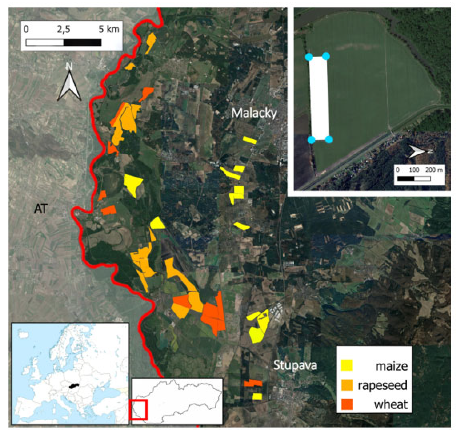
2.1. Study Area and Study Sites

The research took place in Záhorie region, western Slovakia, Europe. The study area (250 km2, 140–155 m above sea level) is a flat lowland dominated with open agricultural land (covering ca 70% of the area), represented mainly by intensively cultivated arable fields and, in the western part, by permanent intensive grasslands. The rest of the study area is covered by forests, small rural settlements and two towns (Malacky and Stupava).
Twenty wheat, 19 maize and 19 rapeseed fields were sampled over the years 2019 and 2020 (Figure 1). Some of the fields were sampled in both years; the total number of fields was 35. The average field size was 50 ha (range 17.3–128 ha). In each of the fields, we established a 500 × 100 m study site, with the longest side corresponding to the edge of the field. The minimum distance between the study sites was 500 m.

2.2. Crop Type and Application of Insecticides

Crop type was recorded for each study site, recognizing wheat, rapeseed and maize. For each study site, the date of insecticide application was obtained from the farm keeper.

2.3. Invertebrate Food Availability

Pitfall traps were used to collect invertebrates to assess food availability for breeding birds. The pitfall trap was a plastic container with a volume of 500 mL and a diameter of 8 cm. Each trap was placed on the ground. The top of the container reached the ground surface, enabling the collection of invertebrates moving into the trap. Every trap was under a metal roof to protect the contents from rainfall. Monopropylene glycol was used in the traps to fix the material.
Two pairs of traps were placed along the shorter side of each study site: one pair at a distance of 1 m and one pair at a distance of 100 m from the field edge (Supplementary Figure S1). The field work took place from April to June and the pitfall traps were left exposed for 14 days each month. This period was selected because it represents the main part of the breeding season for farmland birds in Central Europe. Due to agrotechnical work connected with sowing in maize fields, the traps were not installed before May in this crop type. The contents of both traps within each pair were pooled into one sample, i.e., every study site was characterized by one sample collected at a distance of 1 m (position edge) and another one collected at a distance of 100 m from the edge (position center) separately for each month. Invertebrates were subsequently determined and counted in the laboratory to the level of higher taxonomic groups, mostly orders (Coleoptera, Diptera, Hymenoptera, Araneae, Orthoptera, Heteroptera, Diplopoda, Isopoda, Opiliones, Collembola, Chilopoda, Acari, Lumbricidae, Nematoda, Dermaptera, Stylomatophora, Lepidoptera, Neuroptera, Pseudoscorpiones, Blattodea, Mecoptera and insect larvae). Necrophagous Coleoptera species were removed from the samples before further processing, as their presence and quantity were influenced by the contents of the trap itself. The samples were dried in drying cabinets at 80 °C for 12 h and subsequently weighted with a precision balance (to the level of a thousandth of a gram). For further analysis, the data on invertebrates were expressed using three different variables for each sample: abundance (number of invertebrate individuals), biomass (dry weight) and diversity (Shannon–Weaver index on the relative abundance of respective invertebrate taxa).

2.4. Vegetation Structure

We recorded two vegetation structure characteristics at the study sites: crop height (in cm) and crop cover (in %). Crop height and cover were measured in the area near individual pitfall traps. Specifically, a 1 × 1 m square was established around each trap, within which the cover was estimated by eye as a percentage of the land covered by vegetation (at the scale with the 5% steps, i.e., 0%, 5%, 10%, etc.). Height was determined as the average of measurements at 4 random points within the square. At each study site, the data on vegetation structure collected in the 1 × 1 m squares near the pitfall traps were averaged for the distance 1 m and 100 m from the field edge, respectively (see the details on pitfall trap location above). As a result, we obtained mean crop height and mean crop cover in these positions with respect to the field edge at individual study sites.

2.5. Statistical Analysis

2.5.1. Vegetation Structure

Vegetation structure was examined in three sets of analyses. First, we compared crop height and cover as respective response variables among different crop types, where crop type was considered as a fixed-effect explanatory variable with three levels corresponding to wheat, rapeseed and maize. These relationships were tested by separate generalized linear mixed models (Gaussian error structure, identity link function) run for every month (i.e., April, May and June) using the package ‘glmmTBM’ [34] of the R 4.1.2 software [35]. In each model, the random effects part contained field identity and year as random intercepts. Each response variable was log-transformed before the analysis to improve normality. When the generalized linear mixed model indicated a significant effect of crop type, we applied Tukey’s post-hoc test to assess the differences among respective levels of the explanatory variable (package ‘multcomp’ [36]).
In the second set of analyses, we evaluated changes in crop height and cover during the season. For this purpose, we used crop height and cover as respective response variables related to months as an ordinal fixed-effect explanatory variable. We ran a separate generalized linear mixed model for every crop type (i.e., wheat, rapeseed and maize). The error structure and random effects were the same as in the first analysis set.
In the third set of analyses, we compared crop height and cover between the field edge and the center. For this purpose, we pooled the data from all months and composed a separate model for each crop type. We used generalized linear mixed models (Gaussian error structure, identity link function) with crop height and cover as respective response variables and position within the study site as a fixed-effect explanatory variable, with two levels corresponding to position-edge and position-center. Random effects, variable transformations and post-hoc testing were the same as in the first set of analyses.
Since maize fields did not have vegetation and were not sampled for invertebrates in April, we did not include April data from maize fields in all sets of analyses.

2.5.2. Invertebrate Food Availability

Invertebrate food availability was expressed using three different measures, namely abundance, biomass and diversity (see Section 2.2 Invertebrate Food Availability above), and these measures served as respective response variables in all models. Abundance and biomass were log-transformed to improve normality, whereas diversity had a normal distribution without transformation. We used the same modeling approach to compare the respective measures of food availability among different crop types, changes during the season and between field edge and center as we applied to the analysis of vegetation structure.
To compare taxonomic composition among respective crops, months and positions within the focal fields, we used redundancy analysis (RDA, package ‘vegan’ [37]). RDA was run separately for invertebrate abundance and biomass. In each of these RDAs, invertebrate taxa were respective response variables and crop type, month and position were explanatory variables. Year was included as a covariate to take the repeated sampling of some fields in both years into account.

3. Results

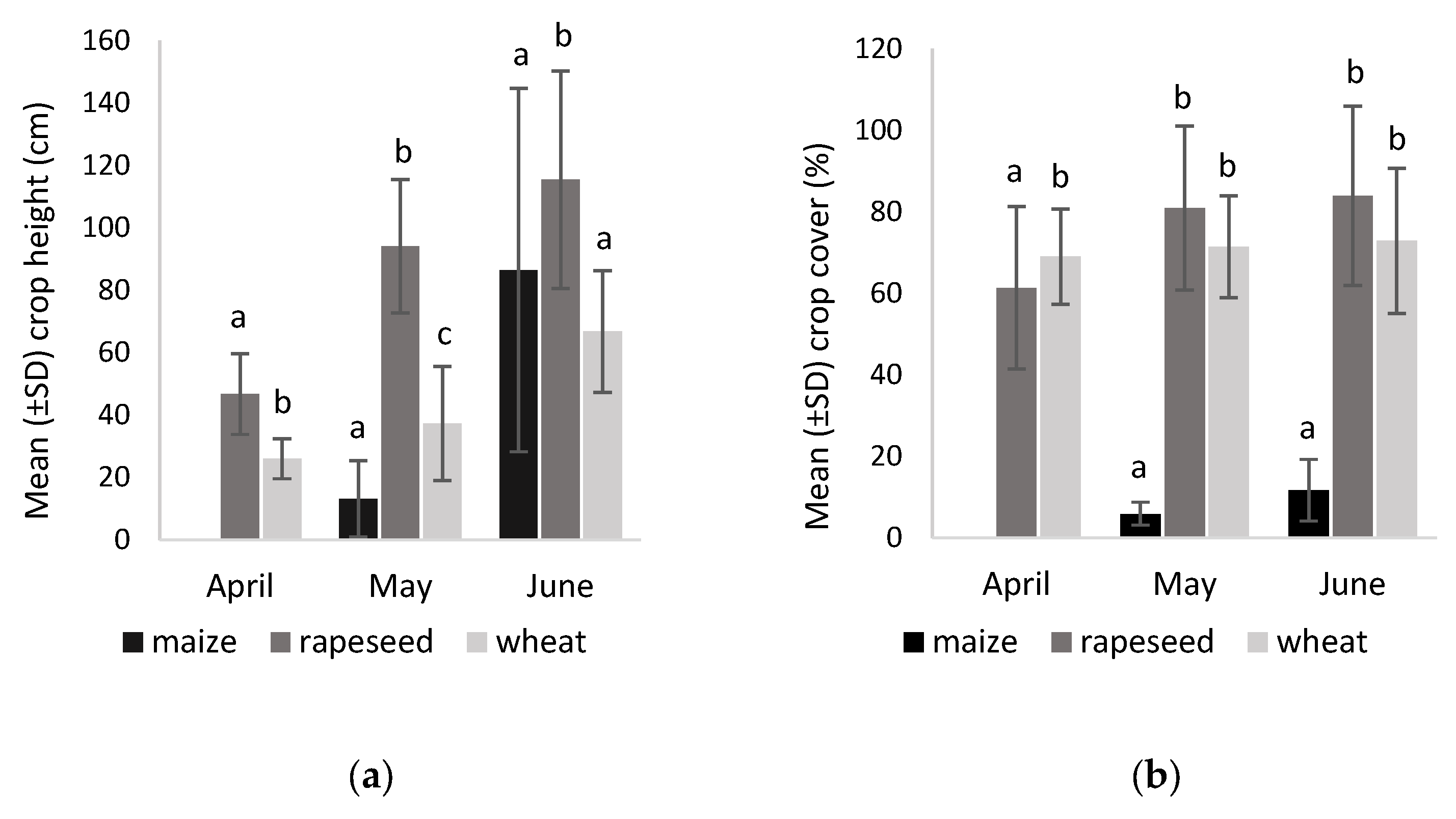
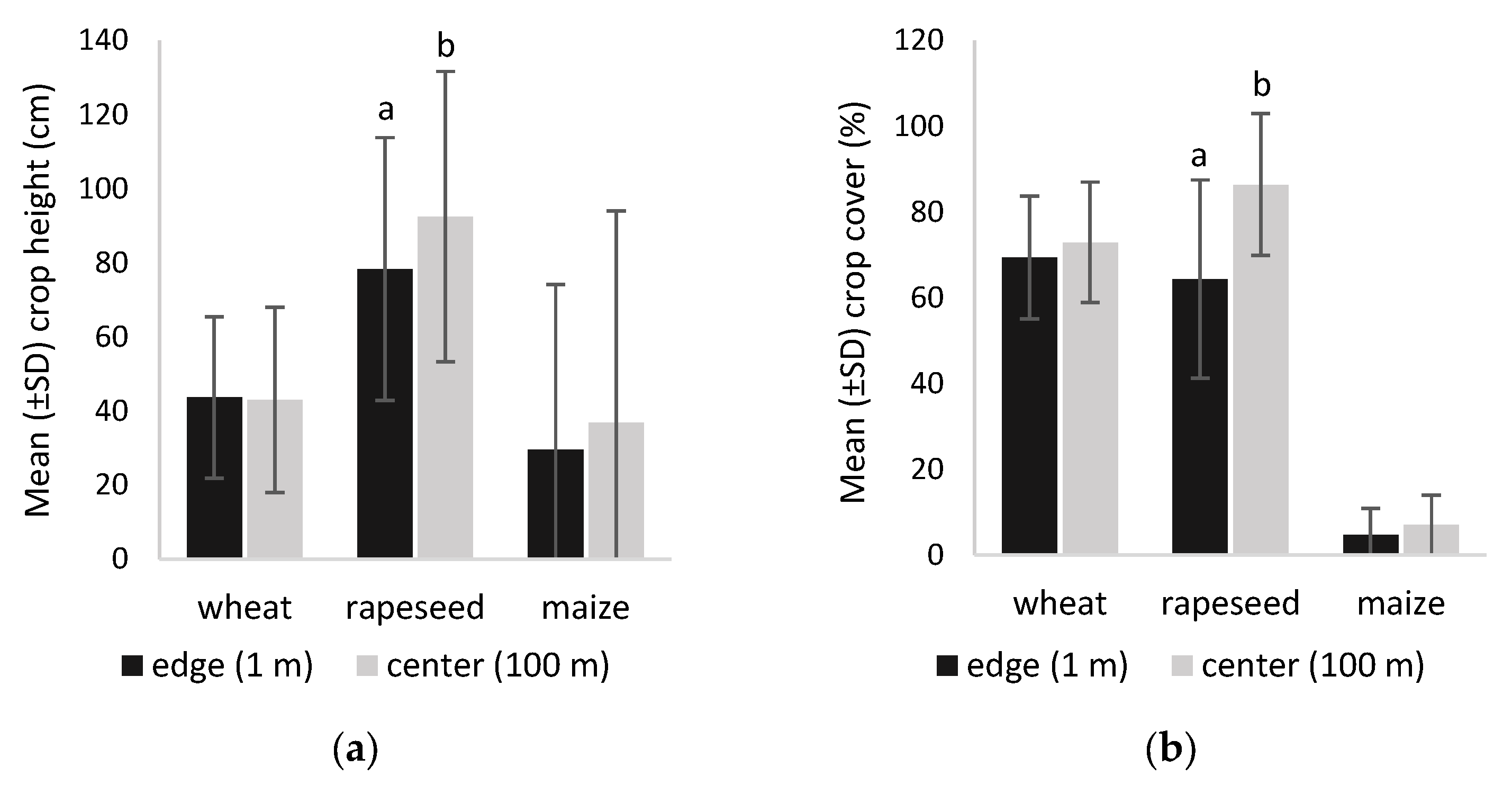
3.1. Vegetation Structure

In every month, the studied crops differed significantly in their height (April: χ2 = 136.71, p < 0.001; May: χ2 = 447.73, p < 0.001; June: χ2 = 30.79, p < 0.001), as well as in their cover (April: χ2 = 5.79, p = 0.016; May: χ2 = 1161.84, p < 0.001; June: χ2 = 469.37, p < 0.001). Maize had zero height and cover in April and low values of both measures were still observed in May (height 0–25 cm, cover 0–10%), which resulted in great differences in comparison with the other crops at that time (Figure 2a). From May to June, maize markedly increased its height (χ2 = 115.05, p < 0.001) reaching 5–200 cm in June and being not significantly different from wheat (50–85 cm, Figure 2a). Its cover remained very low (up to 20%, Figure 2b) even in June, although it still increased significantly over the season (χ2 = 21.08, p < 0.001). Rapeseed also increased its height (χ2 = 154.56, p < 0.001) and cover (χ2 = 17.31, p < 0.001) over the season. It was the tallest crop in all months (reaching the maximum of 150 cm in June, Figure 2a) and had a high coverage, similar to wheat (60–100 %) in all months (Figure 2b). Wheat height progressively increased through the season (χ2 = 193.56, p < 0.001), reaching a maximum of 100 cm in June (Figure 2a). However, its cover remained constant (χ2 = 0.80, p = 0.372) and was relatively high (around 70%) throughout the season (Figure 2b).
There was no difference in the height (χ2 = 0.30, p = 0.582) and cover (χ2 = 1.88, p = 0.170) between the center and edge parts of the study sites in wheat (Figure 3) and the same applied for both height (χ2 = 0.25, p = 0.619) and cover (χ2 = 2.24, p = 0.135) in maize (Figure 3). Only in the case of rapeseed, height (χ2 = 4.20, p = 0.041) and cover (χ2 = 28.50, p < 0.001) had significantly lower values at the edge of the study sites than in the center (Figure 3).

3.2. Insecticide Applications

There were considerable differences in the number and timing of insecticide applications across the studied crops. In maize, insecticides were not applied even once during the observed period. In wheat, on the other hand, insecticides were applied at the beginning of each monitored month (April—June). In rapeseed, insecticides were applied in March (before the start of monitoring), in the first half of April and, in 2019, in the first half of May (Table 1).

3.3. Invertebrate Food Availability

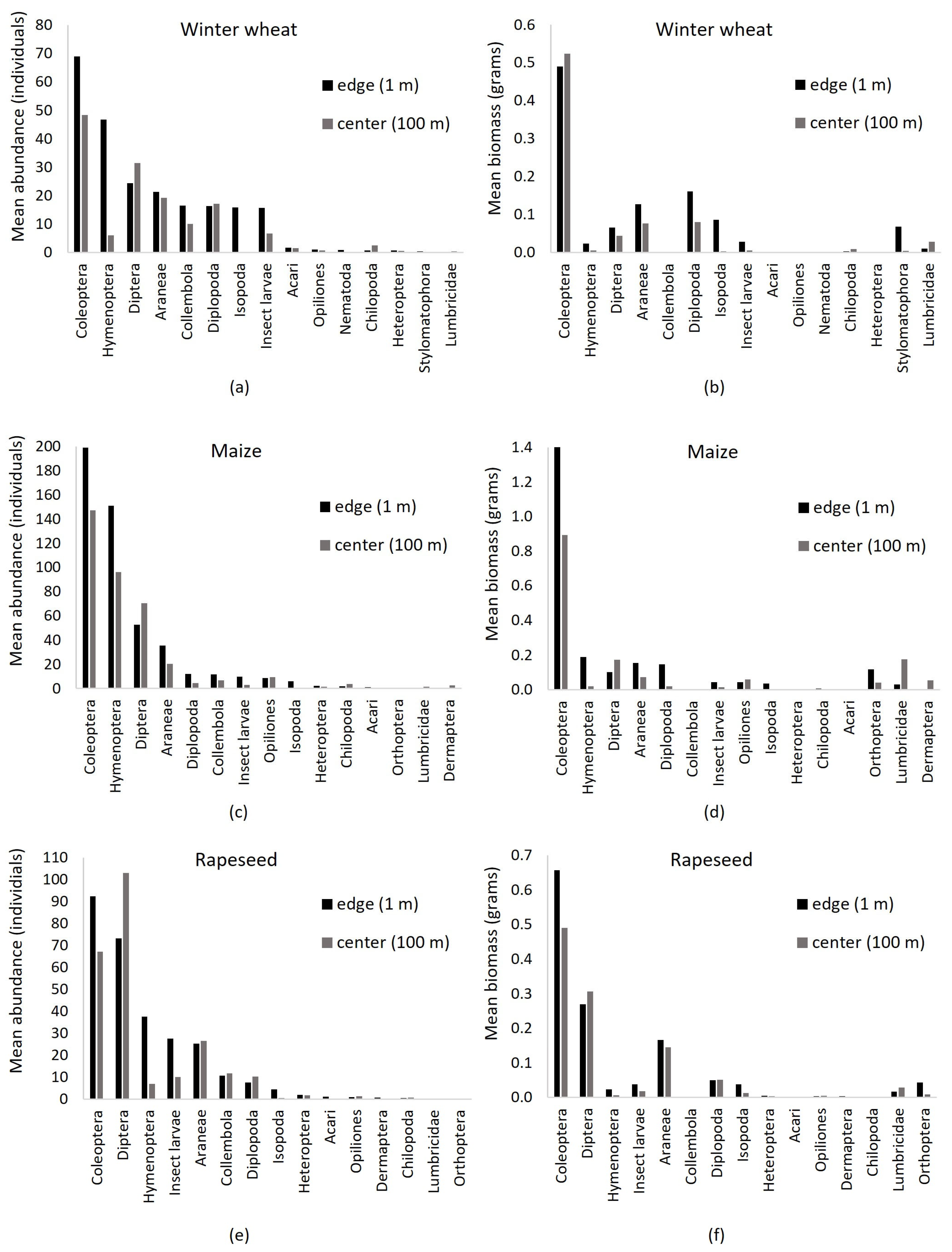
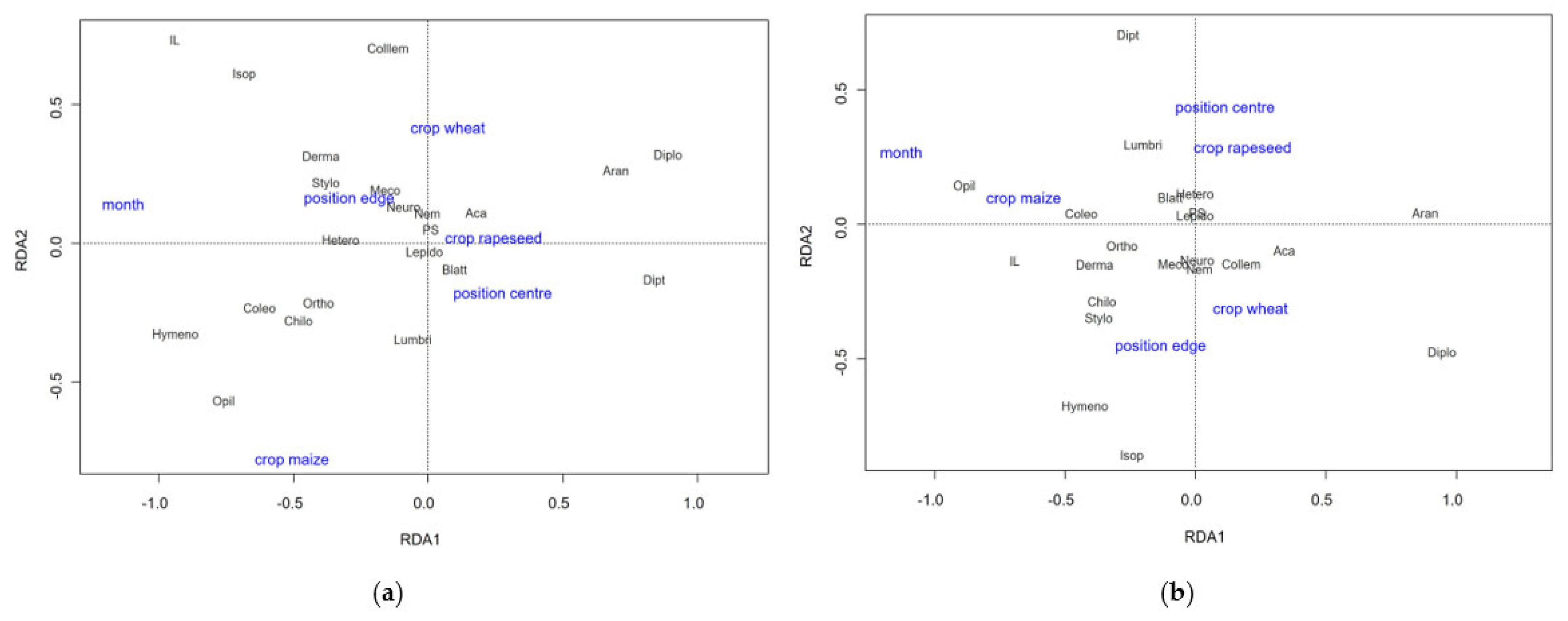
3.3.1. Taxonomic Composition

In total, 76,777 individuals of 22 taxonomic groups of invertebrates were determined, with Coleoptera, Diptera and Araneae predominating across all three crops irrespective of whether abundance or biomass is considered (Figure 4). In all crops, the relative representation of some taxa differed markedly, depending on whether we considered abundance or biomass. Hymenoptera, which was represented mainly by ants, had high abundance, but due to the small weight of individual specimens, they formed only a very small part of the total biomass. In wheat, this was also true for Diptera (Figure 4a,b) and in rapeseed for insect larvae (Figure 4e,f). Stylommatophora, Lumbricideae and Orthoptera (e.g., mole crickets), in contrast, were recorded in small numbers of individuals, but they constituted a significant part of the total biomass.
In wheat, we recorded most of the invertebrate taxa (21; Figure 4a,b). The most numerous were Coleoptera. Together with 6 other taxa (Diptera, Hymenoptera, Araneae, Diplopoda, Collembola, insect larvae), they represented more than 90% of all individuals. In terms of biomass, more than half were represented by Coleoptera. Together with Diplopoda and Araneae, they made up three-quarters of the total biomass. In rapeseed, unlike other crops, the most numerous taxa were Diptera, together with 5 other groups (Hymenoptera, Araneae, Diplopoda, Collembola and insect larvae); they represented more than 95% of all individuals (Figure 4e). When we focused on biomass in rapeseed, almost 50% was made up of Coleoptera. Together with Araneae and Diptera, they made up almost 85% of the total biomass (Figure 4f). In maize, we recorded 19 invertebrate taxa, but almost 90% of all individuals formed only 4 groups: Coleoptera, Diptera, Hymenoptera and Araneae (Figure 4c). Almost 60% of the biomass was made up of Coleoptera in maize (Figure 4d).
To explore gradients in invertebrate taxonomic composition and to explain these gradients by focal explanatory variables (namely crop type, month and position within the studied fields), RDA was performed separately for abundance and biomass. Each RDA model explained a significant amount of variation in invertebrate taxonomic composition in the studied fields (abundance: adjusted R2 = 13.4%, F = 12.039, p = 0.001; biomass adjusted R2 = 5.2%, F = 8.513, p = 0.001). The effects of the respective explanatory variables on taxonomic composition were significant: crop type (abundance: F = 9.989, p = 0.001; biomass: F = 7.596, p = 0.001), month (abundance: F = 15.562, p = 0.001; biomass: F = 10.441, p = 0.001) and position (abundance: F = 12.617, p = 0.001; biomass: F = 8.418, p = 0.001).
According to the abundance RDA model, the first canonical axis depicting the most important gradient (explaining 7.4% of variation in invertebrate taxonomic composition; F = 24.495, p = 0.001) ordinated the taxa from Diplopoda, Araneae and Diptera at its positive end to Hymenoptera, insect larvae, Opiliones, Isopoda and Coleoptera at its negative end (Figure 5a). The negative end of that gradient was associated with the later phases of the season and the connection to maize, while the positive end to the earlier phases of the season and weakly also to rapeseed and the position in the center of the fields (Figure 5a). The second axis (3.3%; F = 10.909, p = 0.001) showed a gradient from Opiliones, Hymenoptera, Lumbricidae, Chilopoda and Coleoptera at its negative end to insect larvae, Collembola and Isopoda at its positive end (Figure 5a). The negative end was associated with maize and the positive one with wheat and weakly also with the position on the field edge (Figure 5a).
According to the biomass RDA model, the first canonical axis (3.0%; F = 15.747, p = 0.001) depicted the gradient from Opiliones, insect larvae and Coleoptera to the taxa Diplopoda, Araneae and Acari (Figure 5b). The negative end of that gradient was associated with the later phase of the season and the connection to maize, while the positive end was connected to the earlier phase of the season and weakly to rapeseed and wheat (Figure 5b). The second axis (1.8%; F = 9.462, p = 0.001) showed a gradient from Diptera and Lumbricidae to Isopoda, Hymenoptera and Diplopoda, with the negative end associated with field edge position and wheat, and the positive end with rapeseed and field center position (Figure 5b).

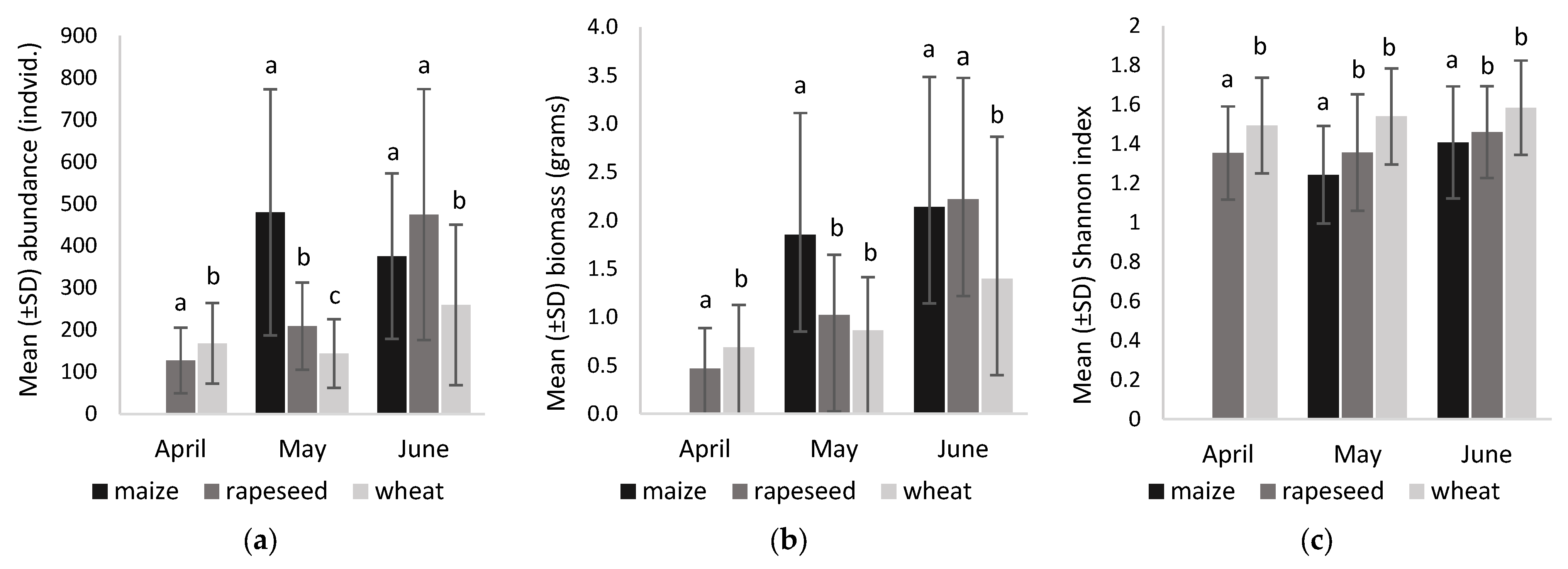
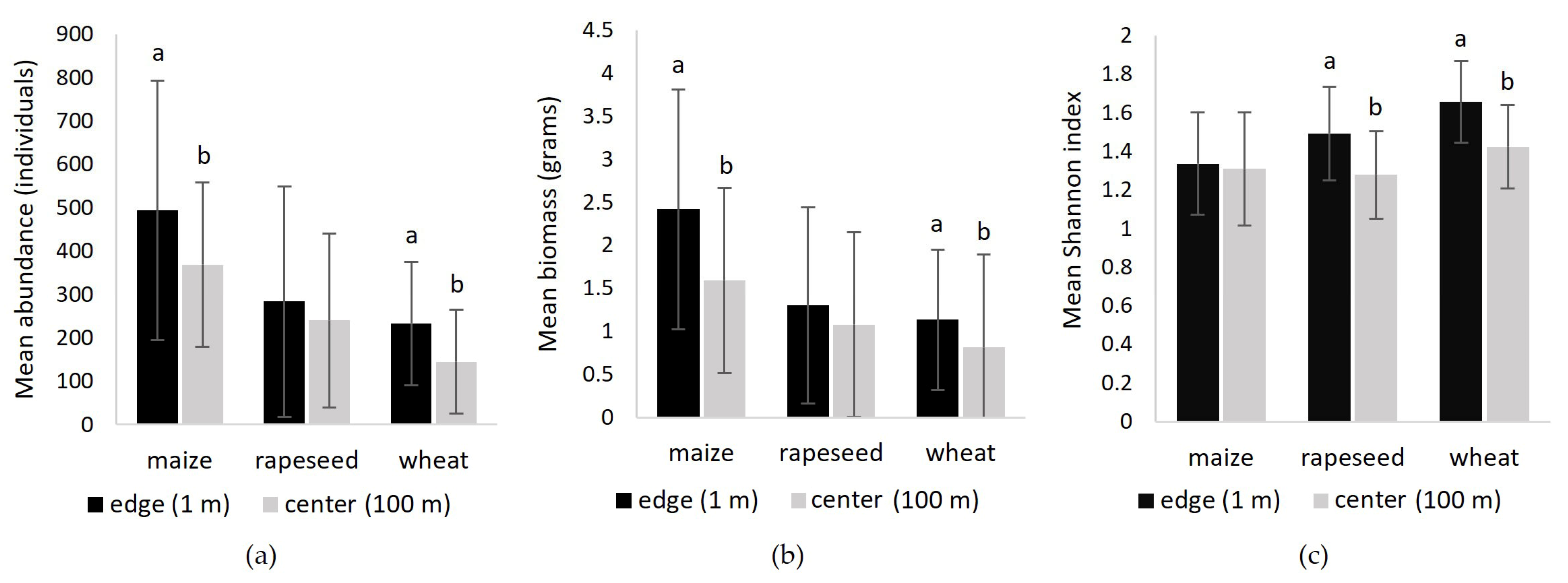
3.3.2. Abundance, Biomass and Diversity

Invertebrate abundance increased during the season in rapeseed (χ2 = 79.754, p ≤ 0.001; Figure 6a). In wheat, the increase was lower but still significant (χ2 = 4.645, p = 0.031; Figure 6a). In maize, the abundance decreased between the observed months (χ2 = 5.738, p = 0.017; Figure 6a).
In April, the per-sample mean invertebrate abundance differed significantly between individual crops (χ2 = 7.666, p = 0.006). Specifically, the mean abundance was 168.0 individuals in wheat and 127.7 individuals in rapeseed (Figure 6a). In May, the significant differences were observed, too (χ2 = 92.818, p ≤ 0.001). Maize had the highest invertebrate abundance (mean = 480 individuals per sample; Figure 6a), followed by rapeseed (209.07 individuals; Figure 6a), whereas wheat hosted the fewest invertebrates (144 individuals; Figure 6a). In June, the model indicated a significant effect of crop type (χ2 = 24.877, p ≤ 0.001), but the differences were less pronounced: rapeseed and maize showed similar abundance (rapeseed: 474.42 individuals, maize: 375.6 individuals), while wheat showed significantly lower values (259.7 individuals; Figure 6a).
Invertebrate biomass increased during the season in rapeseed (χ2 = 85.998, p ≤ 0.001; Figure 6b), less so, but significantly in wheat (χ2 = 5.092, p = 0.024; Figure 6b). In contrast, biomass did not change in maize (χ2 = 1.020, p = 0.313; Figure 6b).
In April, the mean biomass was higher in wheat (0.689 g; Figure 6b) than in rapeseed (0.467 g, χ2 = 9.589, p = 0.002; Figure 6b). In May, the significant effect of crop type on invertebrate biomass (χ2 = 19.510, p ≤ 0.001) was driven by a higher mean value in maize (1.845 g per sample; Figure 6b) than in rapeseed (1.024 g; Figure 6b) or wheat (0.863 g; Figure 6b), which did not differ significantly from each other (Figure 6b). In June, the significant effect of crop type (χ2 = 16.724, p ≤ 0.001) was attributed to the lower invertebrate biomass in wheat (1.399 g; Figure 6b) than both in rapeseed (2.221 g; Figure 6b) and maize (2.142 g; Figure 6b) that showed similar values (Figure 6b).
Invertebrate diversity tended to increase during the season across all crops (Figure 6c), but the changes were modest compared to abundance and biomass. Indeed, a significant increase in diversity was observed only in maize (χ2 = 7.370, p = 0.007) but not in rapeseed (χ2 = 3.203, p = 0.074) and wheat (χ2 = 3.017, p = 0.082).
In April, the diversity of invertebrates was higher in wheat (Shannon index = 1.494; Figure 6c) than in rapeseed (Shannon index = 1.354; diversity: χ2 = 6.673, p = 0.010; Figure 6c). Interestingly, in May, invertebrate diversity showed quite a different pattern from that of abundance and biomass (Figure 6). The significant effect of crop type (χ2 = 25.662, p < 0.001) was due to lower invertebrate diversity hosted by maize (Shannon index = 1.243; Figure 6c) than by the other crops (rapeseed: Shannon index = 1.356, wheat: Shannon index = 1.540; Figure 6c). In June, the pattern of inter-crop differences (χ2 = 9.237, p = 0.010) in invertebrate diversity was similar to that observed in May (Figure 6c), i.e., lower diversity in maize (Shannon index = 1.408; Figure 6c) than in the two other crops (rapeseed: Shannon index = 1.461, wheat: Shannon index = 1.584; Figure 6c).
In all crops, more invertebrates were sampled at the edge of the study sites than at their centers (Figure 7), but the individual crop types showed some differences in this general pattern. Specifically, abundance and biomass of invertebrates were significantly higher near edges in maize (abundance: χ2 = 6.97, p = 0.008; biomass: χ2 = 7.76, p = 0.005; Figure 7a,b) and wheat (abundance: χ2 = 29.07, p < 0.001; biomass: χ2 = 16.06, p < 0.001; Figure 7a,b), but only an insignificant tendency was observed in rapeseed (abundance: χ2 = 2.90, p = 0.088; biomass: χ2 = 3.18, p = 0.075; Figure 7a,b). In contrast, diversity was higher at the edge in wheat (χ2 = 41.18, p < 0.001; Figure 5c) and rapeseed (χ2 = 25.41, p < 0.001; Figure 5c) but not in maize (χ2 = 0.14, p = 0.707; Figure 5c).

4. Discussion

4.1. Patterns in Invertebrate Food Availablity and Vegetation Structure

In this study, we compared several characteristics of invertebrate food availability and vegetation structure among three widespread crops, i.e., wheat, rapeseed and maize, in intensively cultivated large arable fields in southwestern Slovakia. The diversity of invertebrates (expressed as the Shannon index) reached similar levels across all crop types and showed only small changes over the course of the season, i.e., from April to June. In contrast, invertebrate abundance and biomass varied markedly. Specifically, wheat had the lowest abundance and biomass of invertebrates throughout the season. Maize hosted a much higher abundance and biomass compared to other crops in May and maintained high levels of these measures to June. Rapeseed showed very low levels of invertebrate abundance and biomass at the beginning of the growing season, but both of these measures quickly raised as the season progressed, doubled between May and June, and finally reached the same levels as observed in maize.
These seasonal patterns and inter-crop differences can be explained by the interplay of changes in vegetation structure and insecticide application. Insecticides kill both target and non-target invertebrates [17], so their impacts on food availability for farmland birds can be extensive [38]. Here, the low levels of invertebrate abundance and biomass recorded in wheat correspond to the fact that this crop type was also the most frequently treated with insecticides, i.e., in every month of our sampling period. Similarly, maize was the only crop untreated with insecticides in the period of our sampling, which concurs with the high levels of invertebrate abundance and biomass in this crop. The rapid increase in invertebrate abundance and biomass observed in rapeseed from April to June tracks the decreasing frequency of insecticide applications in this crop; the first application occurred just before the start of the sampling period at the end of March, then occurred at the beginning of April, and finally, it was left untreated until the end of June (with the exception of application at the beginning of May in 2019).
The majority of the studied groups of invertebrates increased their total abundance and biomass during the time period. This effect could be explained by the phenological changes of invertebrates during the season, with higher diversity and abundances in the later part of the season [39,40]. At the same time, since invertebrates strongly rely on the vegetation characteristics of their habitats [41,42], seasonal development of the vegetation structure most likely played an important role. Specifically, aboveground vegetation volume rapidly increases with increasing crop height, which results in more habitat and food resources for terrestrial invertebrates [43,44].
This mechanism likely underpins the increase in invertebrate abundance and biomass observed in rapeseed well, corresponding to the marked increase in rapeseed height. Similarly, the growth of wheat from April to June likely contributed to a slight increase in the abundance and biomass of invertebrates over the course of the season, even though the changes in food availability were probably hampered by frequent insecticide applications (see above). On the other hand, seasonal changes in measures of invertebrate abundance, biomass and diversity were decoupled from changes in vegetation height in maize. This crop showed the most drastic increase in height between May and June from all studied crops and was untreated by insecticides at the same time, but the invertebrate abundance and biomass did not increase from May to June. This pattern could be explained by the very low stem density (expressed here by crop cover) observed in maize. Planting maize in low densities is linked to high exposure of topsoil during spring and at the beginning of summer to sunshine. This results in a dry and warm microclimate, which is unsuitable for ground-dwelling invertebrate taxa that prefer wetter and more humid conditions [45]. Therefore, exposure to maize fields likely creates a suboptimal microclimate for most invertebrate assemblages sampled by our traps. These unfavorable microclimatic conditions might have mitigated the usually positive effect of plant height on arthropod biomass and diversity. In addition, the low crop cover per se (being in maize 0–10% in May and up to 35 % in June, i.e., several times lower than in wheat and rapeseed) may also explain low invertebrate diversity in maize because such a simplified habitat structure is typically linked to simplified community composition resulting in low diversity [46,47]. In fact, maize showed the highest inequitability in the invertebrate community composition, with up to 90% of the total abundance represented by only four taxa (Coleoptera, Diptera, Hymenoptera and Araneae). Finally, an important factor responsible for differences in diversity between crops could also be the timing of sowing. Both rapeseed and wheat were winter crops in our case, so fields with these crops could create a longer-term and more stable habitat for invertebrates compared to spring-sown maize [48]. This study also aimed at comparing invertebrate food availability and vegetation structure between field centers and edges. A greater food supply was generally found at the edges of the fields, whereas the vegetation structure did not show increased height and cover closer to the field edge. These results indicate that the higher food supply near the edges could be due to the lower efficiency of insecticide application at the edge of the fields where, for example, lower doses are applied [49]. At the same time, invertebrates can recolonize fields more quickly after treatment from the non-productive vegetation adjacent to the field [50,51,52] resulting in their higher representation near the field edge. The process of recolonization after insecticide treatment, or specifically its absence, could also be the reason why the invertebrate diversity in maize did not differ between the edge and the center of the study site. In this crop, insecticides were not applied, so the effect of recolonization could not be observed in contrast to insecticide-treated wheat and rapeseed. In these treated fields, some groups were completely absent from the center of the study site and may not have been able to quickly recolonize from the edge.
The difference between field margin and interior was also observed in the case of the caught diversity of invertebrate taxa. The majority of groups were more abundant or had higher biomass at the field margins. This could be explained mainly by the spillover effect from adjacent non-productive habitats [40]. Many pollinating groups of insects (e.g., Hymenoptera) in agricultural landscapes depend on food resources from neighboring habitats, increasing their abundance in field margins but with only limited overlap to the internal parts of field blocks [53]. Some ground-dwelling taxa (e.g., Isopoda) are able to persist in such habitats for a long time [54] but due to their worse dispersal abilities [55] altogether with frequent disturbances in the fields, they probably can disperse to the field centers only to a limited extent. In contrast to the field margins, the field interior with dens and spacious crop stands probably forms more stable and humid conditions. The dense and tall vegetation cover is preferred by more mobile ground-dwelling detritivores [40] and can be more attractive to smaller decomposing Diptera and their predators [43]. These links could explain higher abundances of Diplopoda, Diptera and Araneae in the samples from field centers.
Similar effects can also probably explain the differences in invertebrate diversity between crops. While denser stands of wheat and rapeseed were inhabited more by detritivorous ground-dwellers (Collembola, Diplopoda, Isopoda), decomposers (Diptera) and predatory Araneae, the maize form more sparse stands well penetrated to mobile Hymenoptera or larger Coleoptera, especially larger Carabids.

4.2. Implications for the Possibilities of Farmland Bird Occurrence

From the perspective of the bird diet, all groups of invertebrates captured at our study sites were used by the farmland bird species. In general, the most important taxa for adult birds and chicks in the breeding season are adult and larval Coleoptera, adult Hemiptera, adult and larval Lepidoptera, adult and larval Diptera, Hymenoptera, Araneae, Opiliones and Orthoptera [56,57]. However, invertebrate taxonomic composition is of minor importance in contrast to overall food abundance, biomass or food accessibility [58].
When choosing breeding territories, ground-nesting insectivorous farmland birds use a number of factors to assess habitat quality [59]. These factors include vegetation structure and food availability [22]. The vegetation structure plays a primary role in the selection of nesting places, when many species, such as Yellow Wagtail (Motacilla flava) or Corn Bunting (Emberiza calandra), preferentially settle in denser sward to hide nest from predators [60,61], while some others have well-developed antipredator behavior, such as Skylark (Alauda arvensis) or Northern Lapwing (Vanellus vanellus), select open and relatively sparsely vegetated ground [62,63,64,65]. Invertebrates are a key component of the farmland bird diet, not only for obligatory insectivorous species, such as Yellow Wagtail, but also many species mainly herbivorous but supplementing their diet with insects during the reproductive season, such as Grey Partridge (Perdix perdix) [56].
Due to the very different structure of the vegetation and its development during the season, each of the studied crops could create a suitable environment in different parts of the breeding season for different bird species. Wheat forms the most important breeding habitat for farmland birds on arable land in Europe [21,65,66,67]. Based on literature information about farmland bird habitat preferences e.g., [36,37,38], the stand structure in this crop recorded in the study area met such preferences for the longest period from all studied crops. For example, it created suitable conditions in the first half of the Skylark nesting period, when its preferences for height and coverage [20,65,68,69,70,71,72] well corresponded to the values recorded on our study sites in April. On the other hand, in June, the wheat height reached up to 100 cm at 100% density, which most farmland species probably cannot use anymore [73,74].
Maize was very low and sparse at the beginning of the season and agrotechnical processing of the fields occurred at that time, which for many species of birds does not allow a safe placement of the nest [20,75]. However, some birds that prefer low vegetation or bare soil can colonize maize fields at that time, which may be the case with Lapwing [76] or Stone-curlew (Burhinus oedicnemus) [63,77]. At later stages of the season, maize no longer met the preferences of the farmland bird species [63,65,68,78].
In contrast to the sparsely vegetated maize fields, rapeseed formed very dense stands from the beginning of the season and reached an average height of over 1 m during the season. Rapeseed is thus not frequently used for nesting ground-dwelling farmland birds, especially at the end of the season [20]. In the beginning, however, it can suit several species, such as Skylark and Yellow Wagtail [20,68,79,80].
Although wheat was the most suitable crop in terms of vegetation structure, there was the most limited food supply throughout the season in terms of invertebrate abundance and biomass, reducing wheat suitability for insectivorous farmland birds. In addition, the use of invertebrates as food for farmland birds can be negatively affected by a relatively high and dense sward in this crop, especially at the end of the season. This can make food less accessible [22]. Birds that use winter wheat for nesting also often prefer low stands with bare soil for foraging, as applies to Skylark [65,69] or Yellow Wagtail [60,81,82]. Several studies have described the preferential use of tramlines for foraging when crops are too dense, even in cases where there is less food than in the crop [30,69].
Rapeseed, on the other hand, had significantly larger invertebrate abundance and biomass compared to wheat, which continuously increased throughout the season, likely due to the absence of insecticide applications. However, as with wheat, the structure of the stand may prevent birds from using the food potentially supplied by this habitat. Rapeseed fields reached 100% cover and a very high height already in May, which probably makes them less suitable for foraging in many farmland bird species. However, birds can compensate for this inaccessibility by using various defects in the vegetation or tactor tracks [45].
Compared to other studies, maize came out as a relatively food-rich habitat, but this could be due to our sampling method based on pitfall traps. When using a sweep net or D-vac, maize was reported to be worse compared to other crops in other studies [83]. It remains an open question which of the methods samples the food supply in a more appropriate way with respect to bird foraging techniques. In any case, a sparse stand of maize could serve as a farmland foraging habitat in areas where other very dense stands occur.
In our study, a greater and more diverse food supply was found at the edges of the fields. This corresponds with the preferential use of such food-richer habitats in various farmland bird species [29,30,31]. However, the ability of birds to use them may depend on the distance at which their nests are located. For example, in Skylark, its use of field edges dropped sharply if the nest was located in a distance longer than 100 m. [31]. This may have serious implications for the potential use of the food-rich field edges by insectivorous farmland birds in the conditions of excessively large fields occurring in our study area or elsewhere in Central and Eastern Europe. If birds use the center of a 50 ha large field for breeding, they may not be able to benefit from an enhanced food supply at the edge of the field. Therefore, the large field size greatly reduces the availability of such a suitable habitat at the landscape scale.

5. Conclusions and Conservation Implications

From the results of our study, we can conclude that for most typical European ground-nesting insectivorous farmland bird species potentially occurring in our study area, the vegetation structure of the three focal widespread crops provides suitable conditions for nesting only during part of their breeding season and seemingly deteriorates toward its end. Such an unsuitable vegetation structure may, for example, prevent birds from laying second or third clutches. From the invertebrate food supply perspective, we recorded some food-rich habitats, such as maize in May or rapeseed in June. However, the vegetation structure on those sites was not suitable for most ground-foraging birds, making the cover too sparse for nesting (maize) or food likely inaccessible (rapeseed). Wheat provided the most reduced food supply in terms of invertebrate abundance and biomass, likely due to frequent insecticide applications in these fields. Therefore, even though wheat offers the most suitable habitat for ground-nesting insectivores in terms of vegetation structure, this benefit is compromised by food shortages. Improved invertebrate food availability close to the field edges may partly compensate for this deficiency. However, excessive field size, leading to expected fitness costs for birds, effectively reduces the conservation potential of field edges at both local and landscape scales. Based on these findings, conservation measures should include reducing field sizes, limiting the use of pesticides (e.g., by promoting organic farming) to improve food supply, and cultivating spring types of cereals to improve vegetation structure. We are convinced that these measures would have a positive impact on parts of Central and Eastern Europe covered by agricultural areas similar to the ones we studied here.

Supplementary Materials

The following supporting information can be downloaded at: https://www.mdpi.com/article/10.3390/d15040524/s1, Figure S1: Sampling of the studied fields by study sites and pitfall traps.

Author Contributions

Conceptualization, A.H. and J.R.; methodology, A.H., J.R. and T.K.; formal analysis, A.H.; investigation, A.H.; resources, A.H. and J.R.; data curation, A.H.; writing—original draft preparation, A.H.; writing—review and editing, J.R. and T.K.; visualization, A.H.; supervision, J.R.; funding acquisition, A.H. and J.R. All authors have read and agreed to the published version of the manuscript.

Funding

This research was funded by the Charles University Grant Agency, Prague, grant number 392322, and by the Czech Science Foundation, grant number 23–07103S.

Institutional Review Board Statement

Not applicable.

Informed Consent Statement

Not applicable.

Data Availability Statement

Data are available upon request from the corresponding authors.

Acknowledgments

We would like to thank Monika Hološková and Jiří Hološka for help with field work, Martin Štrobl and Jakub Cíbik for help with invertebrate determination, Jan Grünwald for help with statistical analysis, and all farmers for providing access to their fields and management of intensity data. Two anonymous reviewers provided helpful comments to earlier drafts of the manuscript.

Conflicts of Interest

The authors declare no conflict of interest.

References

  1. Tilman, D.; Clark, M.; Williams, D.R.; Kimmel, K.; Polasky, S.; Packer, C. Future Threats to Biodiversity and Pathways to Their Prevention. Nature 2017, 546, 73–81. [Google Scholar] [CrossRef]
  2. Şekercioglu, Ç.H.; Mendenhall, C.D.; Oviedo-Brenes, F.; Horns, J.J.; Ehrlich, P.R.; Daily, G.C. Long-Term Declines in Bird Populations in Tropical Agricultural Countryside. Proc. Natl. Acad. Sci. USA 2019, 116, 9903–9912. [Google Scholar] [CrossRef] [Green Version]
  3. Storkey, J.; Meyer, S.; Still, K.S.; Leuschner, C. The Impact of Agricultural Intensification and Land-Use Change on the European Arable Flora. Proc. R. Soc. B Biol. Sci. 2012, 279, 1421–1429. [Google Scholar] [CrossRef]
  4. Outhwaite, C.L.; McCann, P.; Newbold, T. Agriculture and Climate Change Are Reshaping Insect Biodiversity Worldwide. Nature 2022, 605, 97–102. [Google Scholar] [CrossRef] [PubMed]
  5. Reif, J.; Hanzelka, J. Continent-Wide Gradients in Open-Habitat Insectivorous Bird Declines Track Spatial Patterns in Agricultural Intensity across Europe. Glob. Ecol. Biogeogr. 2020, 29, 1988–2013. [Google Scholar] [CrossRef]
  6. Burns, F.; Eaton, M.A.; Burfield, I.J.; Klvaňová, A.; Šilarová, E.; Staneva, A.; Gregory, R.D. Abundance Decline in the Avifauna of the European Union Reveals Cross-continental Similarities in Biodiversity Change. Ecol. Evol. 2021, 11, 16647–16660. [Google Scholar] [CrossRef] [PubMed]
  7. Fraixedas, S.; Lindén, A.; Piha, M.; Cabeza, M.; Gregory, R.; Lehikoinen, A. A State-of-the-Art Review on Birds as Indicators of Biodiversity: Advances, Challenges, and Future Directions. Ecol. Indic. 2020, 118, 106728. [Google Scholar] [CrossRef]
  8. Bas, Y.; Renard, M.; Jiguet, F. Nesting Strategy Predicts Farmland Bird Response to Agricultural Intensity. Agric. Ecosyst. Environ. 2009, 134, 143–147. [Google Scholar] [CrossRef]
  9. Heldbjerg, H.; Sunde, P.; Fox, A.D. Continuous Population Declines for Specialist Farmland Birds 1987–2014 in Denmark Indicates No Halt in Biodiversity Loss in Agricultural Habitats. Bird Conserv. Int. 2018, 28, 278–292. [Google Scholar] [CrossRef] [Green Version]
  10. Bowler, D.E.; Heldbjerg, H.; Fox, A.D.; Jong, M.; Böhning-Gaese, K. Long-term Declines of European Insectivorous Bird Populations and Potential Causes. Conserv. Biol. 2019, 33, 1120–1130. [Google Scholar] [CrossRef]
  11. Eurostat. Agriculture, Forestry and Fishery Statistics: 2020 Edition; Eurostat: Luxembourg, 2020. [Google Scholar]
  12. OneSoil|The Free Platform for Reliable Agricultural Decisions. OneSoil. Available online: https://onesoil.ai/en/ (accessed on 15 November 2022).
  13. Eurostat Data Browser. Available online: https://ec.europa.eu/eurostat/databrowser/explore/all/agric?lang=en&subtheme=agr.apro.apro_crop.apro_cp.apro_cpsh&display=list&sort=category&extractionId=TAG00093 (accessed on 5 October 2022).
  14. Seni, A. Decreasing Insect Biodiversity in Agriculture—Reorient the Strategy to Reverse the Trend for Better Future. Munis Entomol. Zool. 2022, 17, 360–372. [Google Scholar]
  15. Landis, D.A.; Wratten, S.D.; Gurr, G.M. Habitat Management to Conserve Natural Enemies of Arthropod Pests in Agriculture. Annu. Rev. Entomol. 2000, 45, 175–201. [Google Scholar] [CrossRef]
  16. Asteraki, E.J.; Hart, B.J.; Ings, T.C.; Manley, W.J. Factors Influencing the Plant and Invertebrate Diversity of Arable Field Margins. Agric. Ecosyst. Environ. 2004, 102, 219–231. [Google Scholar] [CrossRef]
  17. Ndakidemi, B.; Mtei, K.; Ndakidemi, P.A. Impacts of Synthetic and Botanical Pesticides on Beneficial Insects. Agric. Sci. 2016, 7, 364–372. [Google Scholar] [CrossRef] [Green Version]
  18. Highland, S.A.; Miller, J.C.; Jones, J.A. Determinants of Moth Diversity and Community in a Temperate Mountain Landscape: Vegetation, Topography, and Seasonality. Ecosphere 2013, 4, 1–22. [Google Scholar] [CrossRef]
  19. Gardner, S.M.; Cabido, M.R.; Valladares, G.R.; Diaz, S. The Influence of Habitat Structure on Arthropod Diversity in Argentine Semi-Arid Chaco Forest. J. Veg. Sci. 1995, 6, 349–356. [Google Scholar] [CrossRef]
  20. Hoffmann, J.; Wittchen, U.; Berger, G.; Stachow, U. Moving Window Growth—A Method to Characterize the Dynamic Growth of Crops in the Context of Bird Abundance Dynamics with the Example of Skylark (Alauda arvensis). Ecol. Evol. 2018, 8, 8880–8893. [Google Scholar] [CrossRef] [PubMed] [Green Version]
  21. Hiron, M.; Berg, Å.; Pärt, T. Do Skylarks Prefer Autumn Sown Cereals? Effects of Agricultural Land Use, Region and Time in the Breeding Season on Density. Agric. Ecosyst. Environ. 2012, 150, 82–90. [Google Scholar] [CrossRef]
  22. Wilson, J.D.; Whittingham, M.J.; Bradbury, R.B. The Management of Crop Structure: A General Approach to Reversing the Impacts of Agricultural Intensification on Birds? Ibis 2005, 147, 453–463. [Google Scholar] [CrossRef]
  23. Devereux, C.L.; McKeever, C.U.; Benton, T.G.; Whittingham, M.J. The Effect of Sward Height and Drainage on Common Starlings Sturnus Vulgaris and Northern Lapwings Vanellus Vanellus Foraging in Grassland Habitats. Ibis 2004, 146, 115–122. [Google Scholar] [CrossRef]
  24. Dunn, J.C.; Hamer, K.C.; Benton, T.G. Nest and Foraging-site Selection in Yellowhammers Emberiza citrinella: Implications for Chick Provisioning. Bird Study 2010, 57, 531–539. [Google Scholar] [CrossRef]
  25. Hoste-Danyłow, A.; Romanowski, J.; Żmihorski, M. Effects of Management on Invertebrates and Birds in Extensively Used Grassland of Poland. Agric. Ecosyst. Environ. 2010, 139, 129–133. [Google Scholar] [CrossRef]
  26. Atkinson, P.W.; Fuller, R.J.; Vickery, J.A.; Conway, G.J.; Tallowin, J.R.B.; Smith, R.E.N.; Haysom, K.A.; Ings, T.C.; Asteraki, E.J.; Brown, V.K. Influence of Agricultural Management, Sward Structure and Food Resources on Grassland Field Use by Birds in Lowland England. J. Appl. Ecol. 2005, 42, 932–942. [Google Scholar] [CrossRef] [Green Version]
  27. Romanowski, J.; Zmihorski, M. Selection of Foraging Habitat by Grassland Birds: Effect of Prey Abundance or Availability? Pol. J. Ecol. 2008, 56, 365–370. [Google Scholar]
  28. Sutcliffe, L.M.E.; Batáry, P.; Kormann, U.; Báldi, A.; Dicks, L.V.; Herzon, I.; Kleijn, D.; Tryjanowski, P.; Apostolova, I.; Arlettaz, R.; et al. Harnessing the Biodiversity Value of Central and Eastern European Farmland. Divers. Distrib. 2015, 21, 722–730. [Google Scholar] [CrossRef] [Green Version]
  29. Brickle, N.W.; Harper, D.G.C.; Aebischer, N.J.; Cockayne, S.H. Effects of Agricultural Intensification on the Breeding Success of Corn Buntings Miliaria calandra. J. Appl. Ecol. 2000, 37, 742–755. [Google Scholar] [CrossRef]
  30. Gilroy, J.J.; Anderson, G.Q.A.; Grice, P.V.; Vickery, J.A.; Watts, P.N.; Sutherland, W.J. Foraging Habitat Selection, Diet and Nestling Condition in Yellow Wagtails Motacilla flava Breeding on Arable Farmland. Bird Study 2009, 56, 221–232. [Google Scholar] [CrossRef] [Green Version]
  31. Kuiper, M.W.; Ottens, H.J.; Cenin, L.; Schaffers, A.P.; van Ruijven, J.; Koks, B.J.; Berendse, F.; de Snoo, G.R. Field Margins as Foraging Habitat for Skylarks (Alauda arvensis) in the Breeding Season. Agric. Ecosyst. Environ. 2013, 170, 10–15. [Google Scholar] [CrossRef]
  32. Clough, Y.; Kirchweger, S.; Kantelhardt, J. Field Sizes and the Future of Farmland Biodiversity in European Landscapes. Conserv. Lett. 2020, 13, e12752. [Google Scholar] [CrossRef]
  33. Štatistický Úrad Slovenskej Republiky. Súpis Plôch Osiatych Poľnohospodárskymi Plodinami k 20.5.2020; Štatistický Úrad Slovenskej Republiky: Bratislava, Slovakia, 2020; ISBN 9788081217791.
  34. Brooks, M.E.; Kristensen, K.; van Benthem, K.J.; Magnusson, A.; Berg, C.W.; Nielsen, A.; Skaug, H.J.; Maechler, M.; Bolker, B.M. {glmmTMB} Balances Speed and Flexibility Among Packages for Zero-Inflated Generalized Linear Mixed Modeling. R J. 2017, 9, 378–400. [Google Scholar] [CrossRef] [Green Version]
  35. R Core Team. R: A Language and Environment for Statistical Computing; R Foundation for Statistical Computing: Vienna, Austria, 2021. [Google Scholar]
  36. Hothorn, T.; Bretz, F.; Westfall, P. Simultaneous Inference in General Parametric Models. Biom. J. 2008, 50, 346–363. [Google Scholar] [CrossRef] [Green Version]
  37. Oksanen, J.; Blanchet, F.G.; Friendly, M.; Kindt, R.; Legendre, P.; McGlinn, D.; Minchin, P.R.; O’Hara, R.B.; Simpson, G.L.; Solymos, P.; et al. Vegan: Community Ecology Package. 2020. Available online: https://cran.r-project.org/web/packages/vegan/index.html (accessed on 9 September 2022).
  38. Moreau, J.; Rabdeau, J.; Badenhausser, I.; Giraudeau, M.; Sepp, T.; Crépin, M.; Gaffard, A.; Bretagnolle, V.; Monceau, K. Pesticide Impacts on Avian Species with Special Reference to Farmland Birds: A Review. Environ. Monit. Assess. 2022, 194, 790. [Google Scholar] [CrossRef]
  39. Chapman, J.W.; Bell, J.R.; Burgin, L.E.; Reynolds, D.R.; Pettersson, L.B.; Hill, J.K.; Bonsall, M.B.; Thomas, J.A. Seasonal Migration to High Latitudes Results in Major Reproductive Benefits in an Insect. Proc. Natl. Acad. Sci. USA 2012, 109, 14924–14929. [Google Scholar] [CrossRef] [Green Version]
  40. Knapp, M.; González, E.; Štrobl, M.; Seidl, M.; Jakubíková, L.; Čížek, O.; Balvín, O.; Benda, D.; Teder, T.; Kadlec, T. Artificial Field Defects: A Low-Cost Measure to Support Arthropod Diversity in Arable Fields. Agric. Ecosyst. Environ. 2022, 325, 107748. [Google Scholar] [CrossRef]
  41. Jeanneret, P.; Schüpbach, B.; Pfiffner, L.; Walter, T. Arthropod Reaction to Landscape and Habitat Features in Agricultural Landscapes. Landsc. Ecol. 2003, 18, 253–263. [Google Scholar] [CrossRef]
  42. Štrobl, M.; Saska, P.; Seidl, M.; Kocian, M.; Tajovský, K.; Řezáč, M.; Skuhrovec, J.; Marhoul, P.; Zbuzek, B.; Jakubec, P.; et al. Impact of an Invasive Tree on Arthropod Assemblages in Woodlots Isolated within an Intensive Agricultural Landscape. Divers. Distrib. 2019, 25, 1800–1813. [Google Scholar] [CrossRef] [Green Version]
  43. McCary, M.A.; Jackson, R.D.; Gratton, C. Vegetation Structure Modulates Ecosystem and Community Responses to Spatial Subsidies. Ecosphere 2021, 12, e03483. [Google Scholar] [CrossRef]
  44. Evans, D.M.; Villar, N.; Littlewood, N.A.; Pakeman, R.J.; Evans, S.A.; Dennis, P.; Skartveit, J.; Redpath, S.M. The Cascading Impacts of Livestock Grazing in Upland Ecosystems: A 10-Year Experiment. Ecosphere 2015, 6, 1–15. [Google Scholar] [CrossRef] [Green Version]
  45. Seidl, M.; González, E.; Kadlec, T.; Saska, P.; Knapp, M. Temporary Non-Crop Habitats within Arable Fields: The Effects of Field Defects on Carabid Beetle Assemblages. Agric. Ecosyst. Environ. 2020, 293, 106856. [Google Scholar] [CrossRef]
  46. Southwood, T.R.E.; Brown, V.K.; Reader, P.M. The Relationships of Plant and Insect Diversities in Succession. Biol. J. Linn. Soc. 1979, 12, 327–348. [Google Scholar] [CrossRef]
  47. Woodcock, B.A.; Pywell, R.F. Effects of Vegetation Structure and Floristic Diversity on Detritivore, Herbivore and Predatory Invertebrates within Calcareous Grasslands. Biodivers. Conserv. 2010, 19, 81–95. [Google Scholar] [CrossRef]
  48. Knapp, M.; Štrobl, M.; Venturo, A.; Seidl, M.; Jakubíková, L.; Tajovský, K.; Kadlec, T.; González, E. Importance of Grassy and Forest Non-Crop Habitat Islands for Overwintering of Ground-Dwelling Arthropods in Agricultural Landscapes: A Multi-Taxa Approach. Biol. Conserv. 2022, 275, 109757. [Google Scholar] [CrossRef]
  49. Crop Protection Association Pesticides—Best Practice Guides. Available online: http://adlib.everysite.co.uk/adlib/defra/content.aspx?id=000IL3890W.16NTBWTSU1UU0 (accessed on 9 September 2022).
  50. Vickery, J.A.; Feber, R.E.; Fuller, R.J. Arable Field Margins Managed for Biodiversity Conservation: A Review of Food Resource Provision for Farmland Birds. Agric. Ecosyst. Environ. 2009, 133, 1–13. [Google Scholar] [CrossRef]
  51. Batáry, P.; Holzschuh, A.; Orci, K.M.; Samu, F.; Tscharntke, T. Responses of Plant, Insect and Spider Biodiversity to Local and Landscape Scale Management Intensity in Cereal Crops and Grasslands. Agric. Ecosyst. Environ. 2012, 146, 130–136. [Google Scholar] [CrossRef]
  52. Holland, J.M.; Smith, B.M.; Birkett, T.C.; Southway, S. Farmland Bird Invertebrate Food Provision in Arable Crops. Ann. Appl. Biol. 2012, 160, 66–75. [Google Scholar] [CrossRef]
  53. Zamorano, J.; Bartomeus, I.; Grez, A.A.; Garibaldi, L.A. Field Margin Floral Enhancements Increase Pollinator Diversity at the Field Edge but Show No Consistent Spillover into the Crop Field: A Meta-Analysis. Insect Conserv. Divers. 2020, 13, 519–531. [Google Scholar] [CrossRef]
  54. Tajovský, K.; Hošek, J.; Hofmeister, J.; Wytwer, J. Assemblages of Terrestrial Isopods (Isopoda, Oniscidea) in a Fragmented Forest Landscape in Central Europe. Zookeys 2012, 176, 189–198. [Google Scholar] [CrossRef] [Green Version]
  55. Szlavecz, K.; Vilisics, F.; Tóth, Z.; Hornung, E. Terrestrial Isopods in Urban Environments: An Overview. Zookeys 2018, 801, 97–126. [Google Scholar] [CrossRef] [PubMed]
  56. Holland, J.M.; Hutchison, M.A.S.; Smith, B.; Aebischer, N.J. A Review of Invertebrates and Seed-Bearing Plants as Food for Farmland Birds in Europe. Ann. Appl. Biol. 2006, 148, 49–71. [Google Scholar] [CrossRef]
  57. Wilson, J.D.; Morris, A.J.; Arroyo, B.E.; Clark, S.C.; Bradbury, R.B. A Review of the Abundance and Diversity of Invertebrate and Plant Foods of Granivorous Birds in Northern Europe in Relation to Agricultural Change. Agric. Ecosyst. Environ. 1999, 75, 13–30. [Google Scholar] [CrossRef]
  58. Newton, I. Food-Supply. In Population Limitation in Birds; Academic Press: Cambridge, MA, USA, 1998; pp. 145–189. ISBN 9780125173667. [Google Scholar]
  59. Fretwell, S.D.; Calver, J.S. On Territorial Behavior and Other Factors Influencing Habitat Distribution in Birds. Acta Biotheor. 1969, 19, 37–44. [Google Scholar] [CrossRef] [Green Version]
  60. Bradbury, R.B.; Bradter, U. Habitat Associations of Yellow Wagtails Motacilla flava flavissima on Lowland Wet Grassland. Ibis 2003, 146, 241–246. [Google Scholar] [CrossRef]
  61. Perkins, A.J.; Maggs, H.E.; Wilson, J.D. Crop Sward Structure Explains Seasonal Variation in Nest Site Selection and Informs Agri-Environment Scheme Design for a Species of High Conservation Concern: The Corn Bunting Emberiza Calandra. Bird Study 2015, 62, 474–485. [Google Scholar] [CrossRef] [Green Version]
  62. Galbraith, H. Effects of Agriculture on the Breeding Ecology of Lapwings Vanellus vanellus. J. Appl. Ecol. 1988, 25, 487–503. [Google Scholar] [CrossRef]
  63. Green, R.E.; Tyler, G.A.; Bowden, C.G.R. Habitat Selection, Ranging Behaviour and Diet of the Stone Curlew (Burhinus oedicnemus) in Southern England. J. Zool. 2000, 250, 161–183. [Google Scholar] [CrossRef]
  64. Wakeham-Dawson, A.; Szoszkiewicz, K.; Stern, K.; Aebischer, N.J. Breeding Skylarks Alauda Arvensis on Environmentally Sensitive Area Arable Reversion Grass in Southern England: Survey-Based and Experimental Determination of Density. J. Appl. Ecol. 1998, 35, 635–648. [Google Scholar] [CrossRef]
  65. Wilson, J.D.; Evans, J.; Browne, S.J.; King, J.R. Territory Distribution and Breeding Success of Skylarks Alauda Arvensis on Organic and Intensive Farmland in Southern England. J. Appl. Ecol. 1997, 34, 1462. [Google Scholar] [CrossRef]
  66. Püttmanns, M.; Böttges, L.; Filla, T.; Lehmann, F.; Martens, A.S.; Siegel, F.; Sippel, A.; von Bassi, M.; Balkenhol, N.; Waltert, M.; et al. Habitat Use and Foraging Parameters of Breeding Skylarks Indicate No Seasonal Decrease in Food Availability in Heterogeneous Farmland. Ecol. Evol. 2022, 12, e8461. [Google Scholar] [CrossRef]
  67. Kragten, S.; Trimbos, K.B.; de Snoo, G.R. Breeding Skylarks (Alauda arvensis) on Organic and Conventional Arable Farms in the Netherlands. Agric. Ecosyst. Environ. 2008, 126, 163–167. [Google Scholar] [CrossRef]
  68. Toepfer, S.; Stubbe, M. Territory Density of the Skylark (Alauda arvensis) in Relation to Field Vegetation in Central Germany. J. Ornithol. 2001, 142, 184–194. [Google Scholar] [CrossRef]
  69. Odderskær, P.; Prang, A.; Poulsen, J.G.; Andersen, P.N.; Elmegaard, N. Skylark (Alauda arvensis) Utilisation of Micro-Habitats in Spring Barley Fields. Agric. Ecosyst. Environ. 1997, 62, 21–29. [Google Scholar] [CrossRef]
  70. Donald, P.F.; Evans, A.D.; Buckingham, D.L.; Muirhead, L.B.; Wilson, J.D. Factors Affecting the Territory Distribution of Skylarks Alauda arvensis Breeding on Lowland Farmland. Bird Study 2001, 48, 271–278. [Google Scholar] [CrossRef]
  71. Chamberlain, D.E.; Wilson, A.M.; Browne, S.J.; Vickery, J.A. Effects of Habitat Type and Management on the Abundance of Skylarks in the Breeding Season. J. Appl. Ecol. 1999, 36, 856–870. [Google Scholar] [CrossRef]
  72. Koleček, J.; Reif, J.; Weidinger, K. The Abundance of a Farmland Specialist Bird, the Skylark, in Three European Regions with Contrasting Agricultural Management. Agric. Ecosyst. Environ. 2015, 212, 30–37. [Google Scholar] [CrossRef]
  73. Kirby, W.B.; Anderson, G.Q.A.; Grice, P.V.; Soanes, L.; Thompson, C.; Peach, W.J. Breeding Ecology of Yellow Wagtails Motacilla flava in an Arable Landscape Dominated by Autumn-Sown Crops. Bird Study 2012, 59, 383–393. [Google Scholar] [CrossRef] [Green Version]
  74. Gilroy, J.J.; Anderson, G.Q.A.; Grice, P.V.; Vickery, J.A.; Sutherland, W.J. Mid-Season Shifts in the Habitat Associations of Yellow Wagtails Motacilla flava Breeding in Arable Farmland. Ibis 2010, 152, 90–104. [Google Scholar] [CrossRef]
  75. Fischer, J.; Jenny, M.; Jenni, L. Suitability of Patches and In-field Strips for Sky Larks Alauda arvensis in a Small-parcelled Mixed Farming Area. Bird Study 2009, 56, 34–42. [Google Scholar] [CrossRef]
  76. Durant, D.; Tichit, M.; Fritz, H.; Kernéïs, E. Field Occupancy by Breeding Lapwings Vanellus vanellus and Redshanks Tringa totanus in Agricultural Wet Grasslands. Agric. Ecosyst. Environ. 2008, 128, 146–150. [Google Scholar] [CrossRef]
  77. Green, R.E.; Griffiths, G.H. Use of Preferred Nesting Habitat by Stone Curlews Burhinus oedicnemus in Relation to Vegetation Structure. J. Zool. 1994, 233, 457–471. [Google Scholar] [CrossRef]
  78. Chamberlain, D.E.; Crick, H.Q.P. Population Declines and Reproductive Performance of Skylarks Alauda arvensis in Different Regions and Habitats of the United Kingdom. Ibis 1999, 141, 38–51. [Google Scholar] [CrossRef]
  79. Kragten, S. Shift in Crop Preference during the Breeding Season by Yellow Wagtails Motacilla flava flava on Arable Farms in the Netherlands. J. Ornithol. 2011, 152, 751–757. [Google Scholar] [CrossRef] [Green Version]
  80. Miguet, P.; Gaucherel, C.; Bretagnolle, V. Breeding Habitat Selection of Skylarks Varies with Crop Heterogeneity, Time and Spatial Scale, and Reveals Spatial and Temporal Crop Complementation. Ecol. Modell. 2013, 266, 10–18. [Google Scholar] [CrossRef]
  81. Stiebel, H. Habitat Selection, Habitat Use and Breeding Success of Yellow Wagtail Motacilla flava in an Agricultural Landscape. Vogelwelt 1997, 118, 257–268. [Google Scholar]
  82. Anthes, N.; Gastel, R.; Quetz, P.-C. Bestand und Habitatwahl Einer Ackerpopulation der Schafstelze (Motacilla f. flava) im Landkreis Ludwigsburg, Nordwurttemberg. Ornithol. Jh. Bad. Württ. 2002, 18, 347–361. [Google Scholar]
  83. Westbury, D.B.; Mortimer, S.R.; Brook, A.J.; Harris, S.J.; Kessock-Philip, R.; Edwards, A.R.; Chaney, K.; Lewis, P.; Dodd, S.; Buckingham, D.L.; et al. Plant and Invertebrate Resources for Farmland Birds in Pastoral Landscapes. Agric. Ecosyst. Environ. 2011, 142, 266–274. [Google Scholar] [CrossRef]
Figure 1. Location of the sampled arable fields (maize, rapeseed and wheat) in the study area (main map). Within each sampled field, a 500 × 100 m study site with four pitfall traps (blue circles) was established (upper right inset). The position of the study area in Slovakia and Slovakia in Europe is also shown (lower left insets).
Diversity 15 00524 g001
Figure 2. Comparison of (a) mean crop height and (b) crop cover among crop types in individual months. Vertical lines represent the standard deviation (SD). Superscripts indicate significant differences between the crop types in each month, based on Tukey’s post-hoc tests.
Diversity 15 00524 g002
Figure 3. Comparison of (a) mean crop height and (b) mean crop cover in each crop type at different distances from the edge of the field. Vertical lines represent the standard deviation (SD). Superscripts indicate significant differences between the edge and center for each crop type, based on Tukey’s post-hoc tests.
Diversity 15 00524 g003
Figure 4. Mean (a,c,e) abundance and (b,d,f) biomass of individual taxa in each crop type at two different distances from the field edge. For each crop type, the figure shows the 15 most represented taxa, ordered from the most to the least numerous groups at the field edge.
Diversity 15 00524 g004
Figure 5. Results of the redundancy analyses (RDA) relating invertebrate taxonomic composition, expressed as either (a) abundance or (b) biomass, to crop type (wheat, rapeseed and maize), position within the field (edge and center) and the time of sampling within the season (month). The relationships depicted by the two most important canonical axes (RDA1 and RDA2) in the respective RDAs are shown. Abbreviations—Aca: Acari; Aran: Araneae; Blatt: Blattodea; Coleo: Coleoptera; Collem: Collembola; Derma: Dermaptera; Diplo: Diplopoda; Dipt: Diptera; Hetero: Heteroptera; Hymeno: Hymenoptera; Chilo: Chilopoda; IL: insect larvae; Isop: Isopoda; Lepido: Lepidoptera; Lumbri: Lumbricidae; Meco: Mecoptera; Nem: Nematoda; Neuro: Neuroptera; Opil: Opiliones; Ortho: Orthoptera; PS: Pseudoscorpiones; Stylo: Stylomatophora.
Diversity 15 00524 g005
Figure 6. Comparison of (a) the mean abundance, (b) biomass and (c) Shannon index between crop types in individual months. Vertical lines represent the standard deviation (SD). Superscripts indicate significant differences between the crop types in each month, based on Tukey’s post-hoc tests.
Diversity 15 00524 g006
Figure 7. Comparison of (a) the mean abundance, (b) biomass and (c) Shannon index of individual crop types at different distances from the field edge. Vertical lines represent the standard deviation (SD). Superscripts indicate significant differences between edge and center for crop type, based on Tukey’s post-hoc tests.
Diversity 15 00524 g007
Table 1. Number and timing of insecticide applications in each crop type every year.
MarchAprilMayJune
Maize0000
Rapeseed111 *0
Winter Wheat0111
* Applied only in 2019.
Disclaimer/Publisher’s Note: The statements, opinions and data contained in all publications are solely those of the individual author(s) and contributor(s) and not of MDPI and/or the editor(s). MDPI and/or the editor(s) disclaim responsibility for any injury to people or property resulting from any ideas, methods, instructions or products referred to in the content.

