Abstract
In this study, we propose a mathematical model based on parametric surfaces for the shell morphology of the phylum Mollusca. Since David Raup’s pioneering works, many mathematical models have been proposed for different contexts to describe general shell morphology; however, there has been a gap in the practicality of models that allow the estimation of their parameter values in real specimens. Our model collects ideas from previous pioneering studies; it rests on the equation of the logarithmic spiral, uses a fixed coordinate system (coiling axis), and defines the position of the generating curve with a local moving system using the Frenet frame. However, it improves upon previous models by applying apex formation, rotations, and substantially different parameter definitions. Furthermore, the most conspicuous improvement is the development of a simple and standardized methodology to obtain the six theoretical parameters from shell images from different mollusc classes and to generate useful theoretical morphospaces. The model was applied to reproduce the shape of real mollusc-shell specimens from Gasteropoda, Cephaloda and Bivalvia, which represent important classes in geological time. We propose a specific methodology to obtain the parameters in four morphological groups: helicoidal, planispiral, conic, and valve-like shells, thereby demonstrating that the model offers an adequate representation of real shells. Finally, possible improvements to the model are discussed along with further work. Based on the above considerations, the capacity of the model to allow the construction of theoretical morphospaces, the methodology to estimate parameters and from the comparison between several existing models for shells, we believe that our model can contribute to future research on the development, diversity and evolutionary processes that generated the diversity in mollusc shells.
1. Introduction
The geometrical spiral beauty of mollusc shells and the relationship between some shells and the logarithmic spiral have attracted biologists’, mathematicians’, and artists’ interest for centuries. Descartes first recongnized the logarithmic spiral in 1638 and, 20 years later, Sir Christoper Wren pointed out its relationship with mollusc shells (Thompson [1]). However, the formal mathematical modeling of mullusc shells began with Henry Moseley in 1838 (Moseley [2]) and, some years later, in a more general context, Ernst Haeckel discussed the science of forms or morphology in a systematic way (Porges et al. [3]). Almost a century later, D’Arcy Thompson, following Moseley’s geometrical approach, showed that morphological differences in shells can be accounted for by the variation in three parameters: the constant angle of the spiral, the ratio of the breadth of successive whorls, and the ratio of the growth rates of the outer and inner borders (Thompson [1]), even introducing the concept of the generating curve: “The surface of any shell, whether discoid or turbinated, may be imagined to be generated by the revolution about a fixed axis of a closed curve, which, remaining always geometrical similar to itself, increases its dimensions continually [⋯] ” (Thompson [1], Chapter 11). These observations are the origin of modern morphological studies. Inspired by D’Arcy Thompson’s work and with the aid of computer graphics, David Raup ([4,5,6]) established the basis for modern theoretical morphology to investigate biodiversity processes and evolutionary patterns. Theoretical morphology offers an additional perspective for studying evolutionary concepts using two types of mathematical simulations: the organic form itself and the morphogenetic process that determines morphology (McGhee [7]). The present work is devoted to the first type of simulation using a geometrical study of the organic shape by constructing theoretical morphospaces, where all mathematically possible shapes are represented.
A theoretical morphospace is an n-dimensional space constructed by systematically varying the values of its axes; each axis represents a geometric parameter of the model, which is a morphological trait of the organism of interest ([8,9]). Once the parameters of a given organism are obtained by a measurement process, it can be mapped into the morphospace. Since computer simulations of the model allow to visualize the entire spectrum of existent and non-existent biological forms, morphospaces have become an important tool to explore evolution constraints and disparity in macroevolution processes ([8,9,10,11]). To build a theoretical morphospace, first of all, a geometrical model of the morphology itself is required. The best example is perhaps the coiling shell of molluscs, which is one of the most widely used biological models in the field of theoretical morphology (Dera et al. [12]) and, to a lesser extent, in other kinds of morphological analysis (e. g., morphometrics in Johnston et al. [13]). To define a model of the biological form, it must be taken into account that the parameters used to define it are important not only for reproducing the form but also to understand its variation. A model which describes forms with great precision needs a large number of parameters, which makes difficult the visualization of realized and unrealized forms in the theoretical morphospace (McGhee [7]).
In this work, we are interested in the shell morphology of the phylum Mollusca. In particular, theoretical analysis has been an important tool to understand the mathematical growth in mollusc shells, mainly because the logarithmic symmetry of their spiral can be described by simple and elegant parameters. This property is due to the fact that molluscs grow by depositing new calcareous material to their shell aperture by mantle tissue, and these accretionary growth processes are relatively simple to model mathematically (Savazzi [14]; chapter 2 in [8,15]). Furthermore, the great morphological diversity, their ontogenetic development and their abundance in the fossil record make these organisms a good model for evolutionary, paleobiological and developmental studies (Haszprunar and Wanninger [16]).
Many mathematical models have been proposed in different contexts to describe the general morphology of mollusc shells. The emergence of different mathematical models has been driven by the definition of specific parameters which attend the morphological problem of the study, as well as by the increasing availability of computation and virtual tools. However, in spite of their peculiar mathematical construction, most of the shell models share geometric characteristics which make it possible to carry out comparisons among them. A complete review of the shell models proposed up to the year 2008 can be found in the extensive and interesting reviews [12,17].
In the context of theoretical morphology, in 1966, David M. Raup developed the first formal model and theoretical morphospace for mollusc shells (Raup [18]), which was inspired by D’Arcy W. Thompson’s work (Thompson [1]). Thompson and Raup’s ideas have influenced the geometric-shell models of several morphologists and paleontologists, both inside and outside of the theoretical field. The fundamental idea of Raup’s model is based on the coiling regularity of shells in terms of the self-similar logarithmic spiral and the generative curve (aperture of the shell), where both are localized within a fixed coordinate system considering a coiling axis. Following this geometric idea, there are models which conserve an isometric growth in the shell ([19,20,21,22]), and others which make modifications to generate allometric growth in the shell with changes in the proportions along its coiling ([23,24,25,26,27,28], among others).
The growing tube model is a different geometric construction proposed by Okamoto [29] which has been used to model the shell form more accurately. The concept of his model relies on using differential geometry to describe a circular cross-section (growing mantle edge) in a moving reference system given by the Frenet frame. This idea has been implemented in several shell-dynamic models which focus on reconstructing the morphogenesis of the shell ([14,15,30,31,32,33,34,35], among others).
The parameters of these dynamic models represent the accretionary process of the aperture at each growing step, which can be biologically correlated (e.g., the genetic expression pattern in Shimizu et al. [36]). Despite their morphogenetic meaning, the growing-tube models are rarely used in empirical studies, mainly because it is complicate to measure and estimate their parameters in real shells. A few innovative methodologies have been proposed to solve this problem; for example, in [37,38,39], a method to quantify the parameters of the growing-tube model from 3D CT scanners and 2D shell images was developed, but it is only applicable to coiling gasteropods.
Another group of mathematical models represents the shell surface using both fixed and moving reference systems. The fixed coordinate system corresponds to a three-dimensional space where the logarithmic spiral is rotated about the z-axis or coiling axis, and the non-fixed reference system is established using the Frenet frame, which consists of the unit tangent, normal, and binormal vectors to a curve. This moving frame allows for the incorporation of the generative curve into the model, given a specific orientation at each point along the logarithmic spiral. This geometric construction was introduced by Illert [40], and later Fowler et al. [41] adopted this idea to model realistic shells with the incorporation of ornamentation and pigmentation patterns. Their work presented a comprehensive and well-defined model; however, in the absence of a formal methodology for measuring specimens, the model is only suitable for image visualization purposes (Prusinkiewicz and Fowler [42]). Appropriately, Ashline et al. [43] suggested a method to determinate the model parameters of Fowler et al. [41] in shell specimens; nevertheless, it is limited exclusively to helicoidal shells and requires data from each of the cross-section apertures, which is difficult to acquire from numerous specimens.
Theoretically, all the previously cited models can provide n-dimensional morphospaces with their own proposed n parameters. However, in reality, there is a lack of visualizable morphospaces in which all theoretical shell forms can be observed; some exceptions can be found in [23,28,29,30]. In addition, the empirical use of theoretical models with a moving reference system is limited mainly because of the absence of a practical method to directly estimate the theoretical parameter values for real specimens; some approaches specifically for helicoidal shells are available in [37,39,43].
Considering this operational problem, the aim of this paper is to propose a geometrical model and methodological approach for the quantification of different shell morphologies. Our shell model is similar to the mathematical construction developed by [40,41]; however, it improves upon previous models by applying apex formation, rotation matrices, and substantially different parameter definitions. Furthermore, the most conspicuous improvement results from proposing a simple and standardized methodology to obtain the theoretical parameters and the coiling axis orientation in real shells, as well as to generate visually appropriate and useful theoretical morphospaces for different mollusc classes.
As an application, the model was used to reproduce the shape of real mollusc-shell specimens from Gasteropoda, Cephaloda, and Bivalvia, which represent important classes in geological time. We also propose a specific methodology to obtain the parameters for four morphological groups: helicoidal, planispiral, conic, and valve-like shells, demonstrating that the model offers an adequate representation of real shells. We believe that our model and the generated theoretical morphospaces will motivate future research on the development and evolutionary processes that have generated the diversity in mollusc shells.
2. Materials and Methods
2.1. Materials
Our model can be applied to a wide variety of morphologies in both recent and fossil shells. As an example, it was applied to reproduce the shape of fossil mollusc shells, especially because they present a great diversity in shapes which are the subject of evolutionary studies by the paleontological community, as well as to demonstrate that the proposed methodology can be used even when the specimens are not fully preserved or complete. To test its capacity for reproducing the shape of mollusc shells, we used photographs of fossil specimens from the Invertebrate Paleontology Department collection of the Natural History Museum of Los Angeles County. Real shell specimens representing important classes in geological time, Gastropoda, Cephaloda, and Bivalvia, were chosen. Five morphologically different specimens for each class were selected to obtain a large variation in shell geometry and demonstrate the applicability of the model to helicoidal, planispiral, conic, and valve-like shells.
Photographs of the apertural and apical views were used to measure the parameters for each specimen.The specimens considered and their corresponding catalog number, family, age and location, were as follows.
Asperiscala pacis (LACM 71-175-8, Epitoniidae, Neogene, California); Acteon sullivanae (LACMIP 23768-1, Acteonidae, Cretaceous, California); Lirularia pedroana (LACM 73-10-18, Trochidae, Pleistocene, California); Brachysphingus mammilatus (LACMIP 17190-1, Buccinidae, Eocene, California); Biplica obliqua (LACMIP 10710-4, Ringiculidae, Cretaceous, California); Oregoniceras siskiyouense (LACMIP 8547, Collignoniceratidae, Cretaceous, California); Nautilus aff. N. cookanum (LACMIP 6938, Nautilidae, Eocene, Washington); Cleoniceras (Grycia) susukii (LACMIP 9876, Cleoniceratidae, Cretaceous, California); Shasticrioceras patricki (LACMIP 23014-1, Diplomoceratidae, Cretaceous, California); Baculites boulei (LACMIP 23297-2, Baculitidae, Cretaceous, California); Scelidotoma bella (LACM 60-24-29, Fissureliidae. Pliocene, California); Cucullaea morani (LACMIP 26525, Cucullaeidae, Cretaceous, California); Glycymerita banosensis (LACMIP 9196, Glycymerididae, Cretaceous, California); Indogrammatodon vancouverensis (LACMIP TX 10715-176, Parallelodontidae, Cretaceous, California); Crepidula adunca (LACM 1942-51-5, Calyptraeidae, recent, Oregon).
2.2. The Model
The proposed model collects ideas from several pioneering works which are based on parametric surfaces and a moving reference system, discussed in Section 1; it contains, basically, two terms, which in a compact form can be written as
where:
- (1)
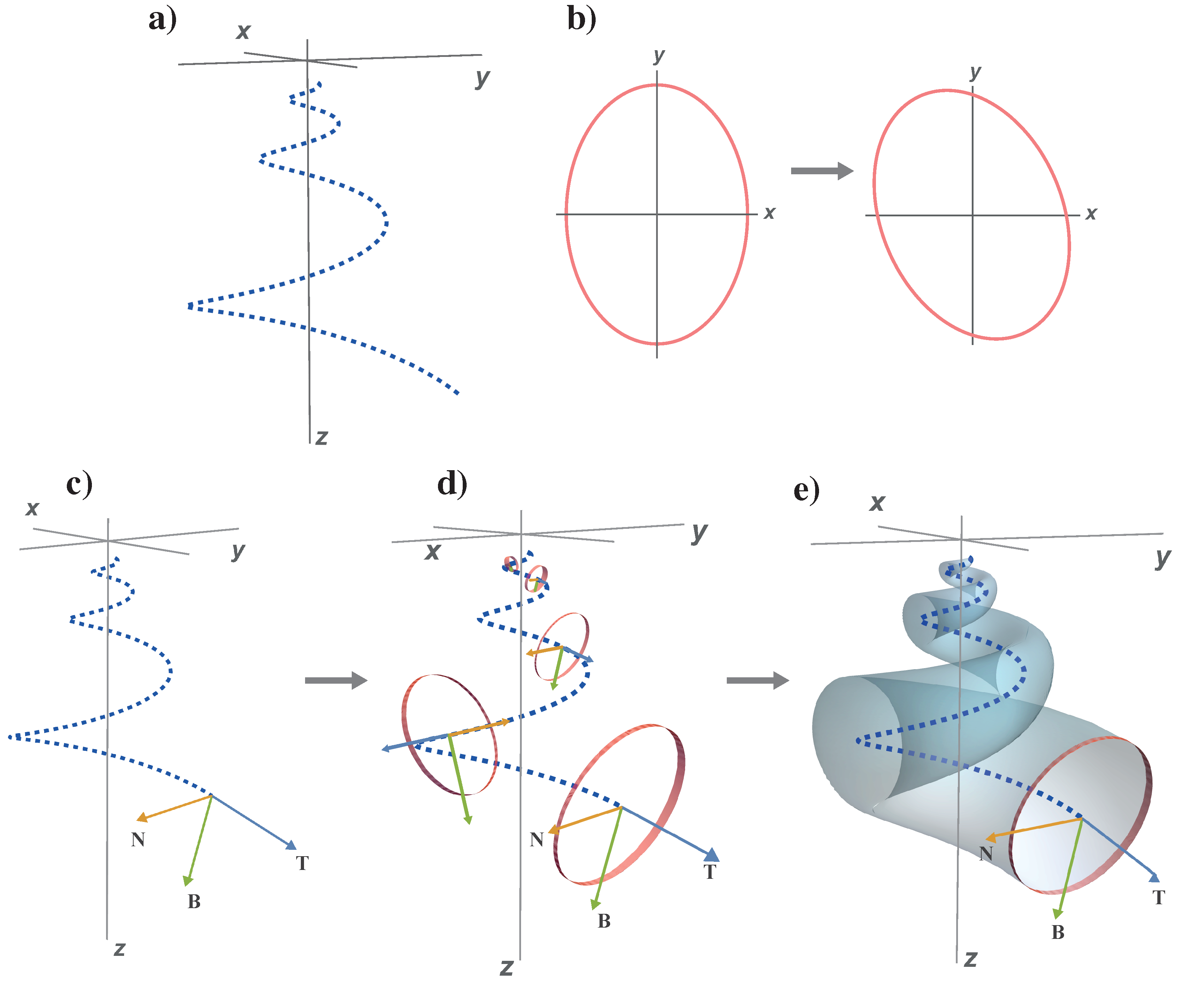
- is a logarithmic spiral curve that unwinds around the z axis, which is referred to as coiling axis (Figure 1a). This curve is defined bywhere b is the expansion rate, d is the horizontal distance to the coiling axis and z is the distance to the plane, that is, the vertical translation.
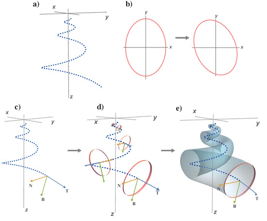 Figure 1. Graphic representation of the elements of the proposed mathematical model: (a) 3D logarithmic spiral in a fixed coordinate system; (b) elliptical generative curve and its rotation into the plane; (c) Frenet frame on the logarithmic spiral; (d) the generative curve moves along the logarithmic spiral using the Frenet frame as a moving reference system; and (e) final geometric shell model.
 - (2)
- is the generating curve which, when moving along , traces out a surface which is the model of the mollusc shell. This generating curve is the aperture whose size increases as it moves along . The equation of the generating curve is obtained through a process described as follows:
- (a)
- The aperture is modeled by an ellipse (Figure 1b), since the aperture of many shells can be approximated by this shape. Its parametric equation in a two-dimensional fixed coordinate system iswhere , and a accounts for the ratio between major and minor axes. To better describe some samples, the ellipse (3) can be tilted by an angle (Figure 1b):Since this aperture moves along , to describe this rotated ellipse in a moving coordinate system, we use the Frenet frame field on (Figure 1c), which is the triple of unitary mutually orthogonal vectors , where , and are the tangent, the normal and binormal vector fields of , respectivelly (Gray et al. [44]). For , given in (2), these vectors are given byIn this local moving frame, the equation of the ellipse (4) located in the plane becomes:The inclination of the aperture with respect to the z axis (the coiling axis) is also an important element to consider because it has been suggested that it has remarkable functional and ecological aspects (Vermeij [45]). If denotes the rotation angle around the axis in the local moving frame, the rotation of (8) produceswhere
- (b)
- Finally, when moving along , the ellipse (8) usually increases its size exponentially as , where the parameter b is called expansion rate, and is the initial aperture size (Figure 1d). This geometrical construction generates a shell model that appears incomplete in the apical area (with an initial aperture ). For modeling convenience, we modified this approach to include a t-dependent factor which allows the tip of the shell to be closed. With this, the final form of the generating curve isNote that if a non-zero aperture size is required, it can be obtained starting from a suitable .
In summary, the model equation that dictates the final surface of the shell (Figure 1e) is:
2.3. Parameters of the Model
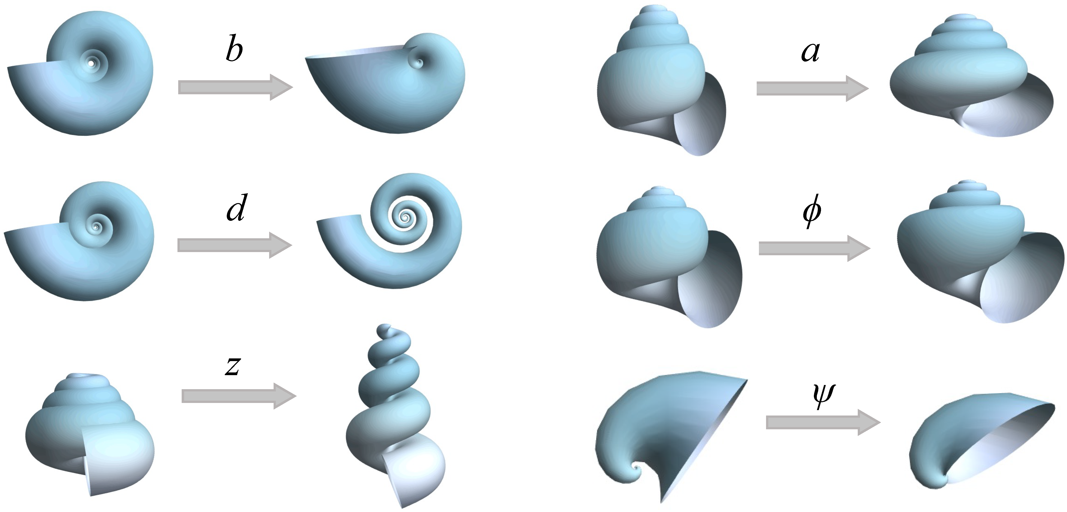
The parametric equation of the shell model (12) contains six dimensionless fixed parameters: b, d, z, a, and . The parameters are listed below, including their range of theoretical values. The effect of each of these parameters on the shell’s shape is described below and shown schematically in Figure 2.

Figure 2.
Graphical description of the effect of variation in the parameters of the proposed mathematical model.
- b
- Whorl expansion rate. It measures how fast the spiral , and, consequently, the generating curve of the shell expands. The range of this parameter is ; corresponds to a torus whereas produces a straight shell.
- d
- Horizontal distance from to the coiling axis. Its range is ; produces an infinitely expanded shell.
- z
- Vertical translation of , that is, the vertical distance from to the plane. Its range is ; dextral coiling is obtained for whereas produces sinistral shells; planispiral shells are obtained with .
- a
- Ratio between the major and minor axes of the ellipse modeling the aperture of the shell. Its range is ; the aperture of the shell can be narrow (), circular (), or wide ().
- ϕ
- Initial tilt angle of the shell aperture (generating curve) before it is located in the Frenet frame (4). Its range is ; at , the initial configuration is obtained.
- ψ
- Is the rotation angle around the axis () in the local moving Frenet frame (Figure 2). To avoid invagination, the considered range is .
The mathematical model proposed here can be modified to generate more realistic shells (e.g., ornamentation and aperture shape), paying the cost of increasing the number of parameters and dimensions of the theoretical morphospaces. Three additional parameters which can be useful for modeling ornamentation (such as ribs) and displacement of the aperture with respect to the coiling axis (a characteristic common in bivalves) are described in the last subsection. The theoretical morphospaces presented in this work are limited to the six parameters presented above for practical applications.
2.4. Estimation of the Parameters
A crucial step in modeling the shape of a given shell is to estimate the six parameter values previously described through measurements from real specimens. Here, we propose a methodology to estimate the value of each of the six parameters using particular measurements on the shell specimen. As we will show, each parameter requires only two measurements to calculate its value in a real shell, which facilitates estimation of the parameter values of the specimens.
It is important to mention that any measurement requires the correct and standard alignment of the shell, which is achieved by first identifying the coiling axis. Therefore, in the following subsections, we propose methodologies for calculating the theoretical coiling axis of a given specimen for the any of the general morphologies of coiling shells: helicoidal (gastropod-like), planispiral (ammonoid-like), and valves (bivalves-like).
2.4.1. Parameter b
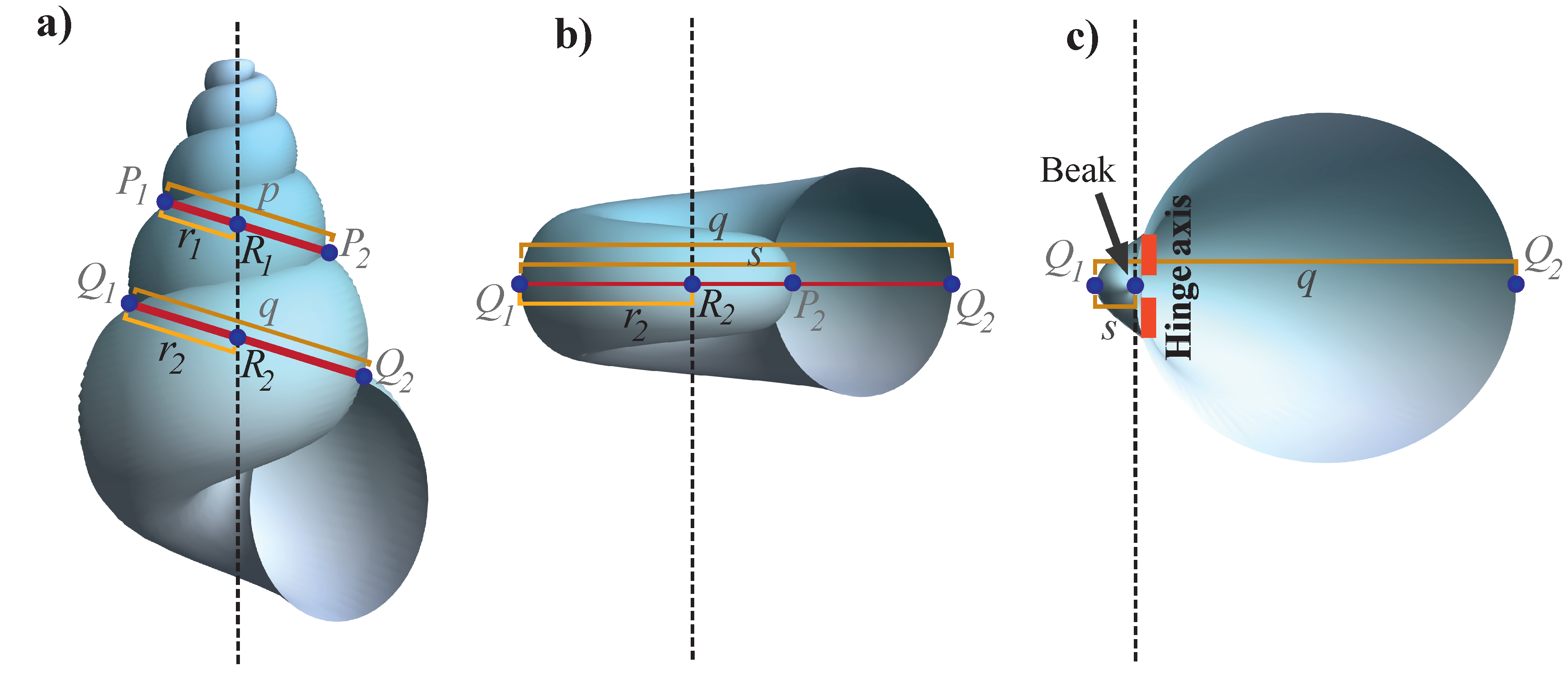
This parameter dictates the general form of the shell; it accounts for the growth rate of both the logarithmic spiral (2) and the aperture or generating curve (11). The expansion rate b can be calculated by measuring the length of two segments and , with magnitudes and , respectively, measured at contiguos whorls; that is, if p is measured at a given t, then q is measured at (Figure 3). In polar coordinates, from the equation of the logarithmic spiral, we have that , , , and , and from the properties of the logarithmic spiral, it can be shown that
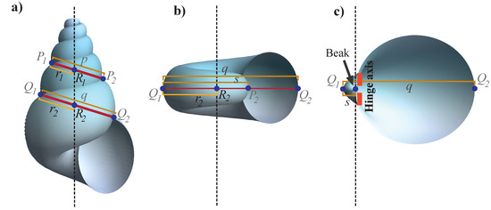
Figure 3.
Measurements required to obtain the parameter b and the theoretical coiling axis in (a) helicoidal shells, (b) planispiral shells, and (c) valve-like shells. Vertical dashed lines represent the coiling axis.
By taking the logarithms on both sides, we obtain
For helicoidal shells, Figure 3a shows some methods for measuring distances p and q. Note that for planispiral shells and valves, point is not visible because it is covered by the following whorls during coiling on the plane. However, it is possible to obtain the distance (Figure 3b,c), and because these two points are separated by half of turn, the equation of parameter b for planispiral shells is . In the case of valve-like shells, the distance s is too small such that point generally coincides with the beak of the umbo. An extra consideration for parameter b can be useful when the specimens are not well-preserved or are incomplete (see Section 2.4.2).
Before describing the method for measuring the other parameters of the model, we describe how to determine the location of the theoretical coiling axis, because it is important to correctly align the shell and, thus, measure the remaining parameters.
2.4.2. Coiling Axis
In general, the coiling axis is not easily located on real shells; sometimes, its location can be approximated with the columella in gastropods, the orthogonal hinge axis in bivalves, or the cross-sections in ammonoids. In the following, we propose methodologies for calculating the theoretical coiling axis of a given specimen of any of the three general shell coiling forms: helicoidal (gastropod-like), planispiral (ammonoid-like), and valves (bivalves-like).
Helicoidal and planispiral shells. The position of the coiling axis can be estimated and displayed from the apertual view. Consider lines and as the union of the suture points of consecutive whorls in Figure 3a,b. Theoretically, the coiling axis passes through these two lines and intersects them at the points and . Therefore, it is necessary to follow the following methodology in order to locate the positions of these two points. If , , and ; due to the properties of logarithmic spirals, we have that . Since , and , then:
Thus, divides p by and, consequently, divides q by the same quantity. Since p and q are measured, and can be determined.
Note that although helicoidal shells require two points, and , to define the coiling axis, for planispiral shells in the apertural view, one point () is sufficient (Figure 3b). The coiling axis (broken line in Figure 3b) must be perpendicular to line ; and are the extreme points of the ventral region of the planispiral shell.
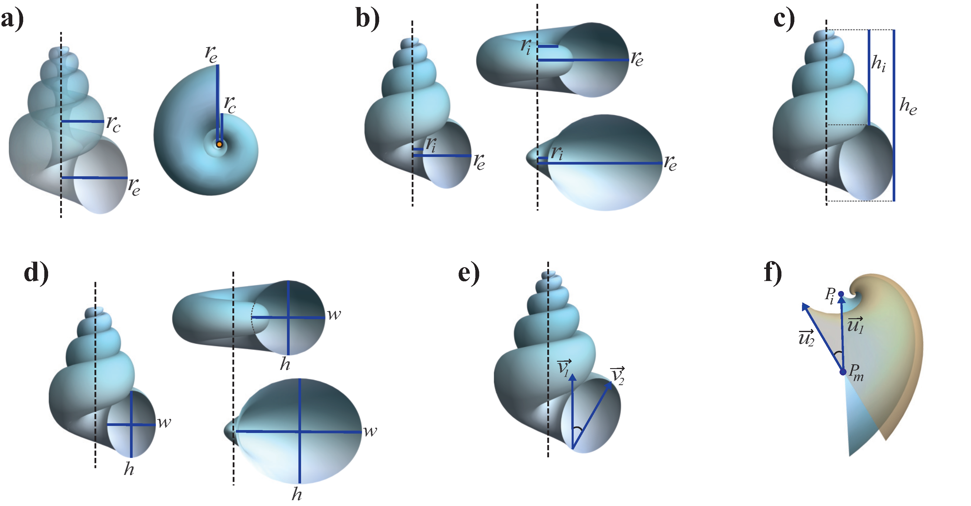
Sometimes, the coiling axis cannot be calculated with the above method if the specimen is not well-preserved, but it can be located in an approximate way with the morphological characteristics of the shell (e.g., columella or umbilicus). In this case, the parameter b can be measured using two linear distances, and , as shown in Figure 4a. Both distances are measured from the coiling axis to the last existing point of the external border of the generating curve, but is located at one whorl less than (Figure 4a); with these measurements, we have for both helicoidal and planispiral shells.

Figure 4.
Measurements required to calculate: (a) parameter b, (b) parameter d, (c) parameter z, (d) parameter a, (e) parameter and (f) parameter (the yellow shape corresponds to ). Vertical dashed lines represent the coiling axis.
Shell valves. Few anatomical structures are distinguishable in the morphology of valve shells because they have high rates of whorl expansion, and shell whorls are not clearly evident. To determine the position of the coiling axis, it is possible to use the same method for the planispiral shell with segments q and s. However, it has been proposed that the coiling axis of valves corresponds to the morphological element of the beak. Therefore, instead of using the logarithmic spiral equation, it is necessary to distinguish the apex of the beak and the hinge axis of the valve (Figure 3c), which are key morphological elements for the correct orientation of the shell in an axis-based framework (Edie et al. [46]).
The apex of the beak represents the early developmental growth of the shell (Carter et al. [47]) and the hinge axis is an imaginary straight line defined by the motion of the valves (Cox et al. [48]). Considering these two morphological elements, the coiling axis is defined as the line that crosses the apex of the beak and is oriented along the hinge axis (Figure 3c).
2.4.3. Parameter d
Parameter d is used to define the logarithmic spiral, and it represents a scaling factor which displaces the curve in the plane (2). From its polar equation , we obtain , where r is the horizontal distance from coiling axis to , which is located at the middle of the generating curve (Figure 1e, dashed line). This distance r cannot be measured in a shell because the visible structures are the ends of the generating curve, and not the inner part of the shell. However, we know that the radius of the generating curve increases exponentially as ; therefore, it is necessary to include a, which is the ratio between the major and minor axes of the ellipse, in the measurement of d. The apex modification of the model shell indicates that the aperture size grows as (11); however, the second term in the parenthesis affects the aperture growth mainly at the beginning of the shell growth, so it can be omitted for the calculus of d. The value of the horizontal distance from the coling axis to and the radius of the generating curve can be obtained using the linear measures and in the specimen (Figure 4b). Both distances are measured on the same whorl. Now, we have that
but , then
Measurements of and can be performed either in the apertural or in the apical view of all the morphologies of shells.
Note that the parameters d and a are linearly dependent (except for , when the generating curve is a circle). This will produce that real mapped specimes (realized forms) fall in a subspace of the complete morphospace; however, since d and a can be varied freely, the unrealized forms are mapped in the complete morphospace.
2.4.4. Parameter z
As for d, the parameter z is a scaling factor for , but along the z axis, which controls the vertical distance along the coiling axis (2). Therefore, the parameter z is calculated by following the same procedure as parameter d, but taking into account that, in this case, the minor axis of the ellipse is 1 so a is not involved. We have that along the z direction ; thus, , where r corresponds to the position of and is the expansion rate of the radius of the generating curve. The distances and in Figure 4c play the same role as and used to calculate the parameter z (Figure 4b), but in the vertical direction; they are measured parallel to the coiling axis, starting from the apex of the shell to the external border of the aperture () and to the internal border of the aperture () at the same whorl. By following the same procedure used to calculate d, we can show that
It should be noted that this parameter is only measurable in lateral or apertural views of helicoidal shells where vertical coiling is visible. For planispiral and bivalves-like shells, .
2.4.5. Parameter a
This parameter modifies the ratio between the major and minor axes of the ellipse that conforms the generating curve (3), and is defined simply as
where w is the whorl width and h the whorl height; h is parallel to coiling axis, whereas w is perpendicular to coiling axis when the aperture is not rotated (Figure 4d); both distances must be measured at the same whorl section.
This parameter is only visible and measurable in the aperture view of shells. It is important to note that in the classic nomenclature for planispiral shells, the whorl height corresponds to the perpendicular distance to the coiling axis and the whorl width is the parallel distance. However, to easily compare shells, the distances h and w were defined in the same way for all shell morphologies (Figure 4d).
2.4.6. Parameter
The angular parameter is the initial rotation of the shell aperture just before it is located in the Frenet frame (4). In a specimen, can be obtained as the angle between the coiling and the vertical axes of the elliptical generating curve. As shown in Figure 4e, to measure this angle two vectors are required: the location of the coling axis , and the vector whose magnitude define the height (h) of the shell aperture . Once measured, the coordinates of these vectors, , is calculated as
where · represents the standard Euclidean inner product. The rotation by is only visible and measurable in the aperture view of shells.
2.4.7. Parameter
This is the second angular parameter used to modify the orientation of the aperture, especially in bivalve-like shells; the measure of two vectors on the specimen, and , are required to calculate it. For a given specimen with a rotated aperture (), the vectors required to calculate are defined as follows. As shown in Figure 4f, has its tail at point , located at the middle of the aperture, and its head at point , located at the dorsal end of the aperture. The second vector is calculated theoretically with its tail at point , and is parallel to the aperture when . Note that is parallel to the normal vector of the moving frame, when . From (6), it is clear that the expression is simplified if the measure is taken at the first turn (), since ; thus, considering only the orientation of the vector, it turns out that . With this, the parameter is calculated as the angle between the measured vector and the calculated vector as:
As the normal vector is determined at , it is important to emphasize that the vector must be measured at a specific orientation of the specimen; the point and the apex of the umbo must be on the same vertical line in the lateral view of the shell (Figure 4f).
2.5. Orthoconic-Like Shells
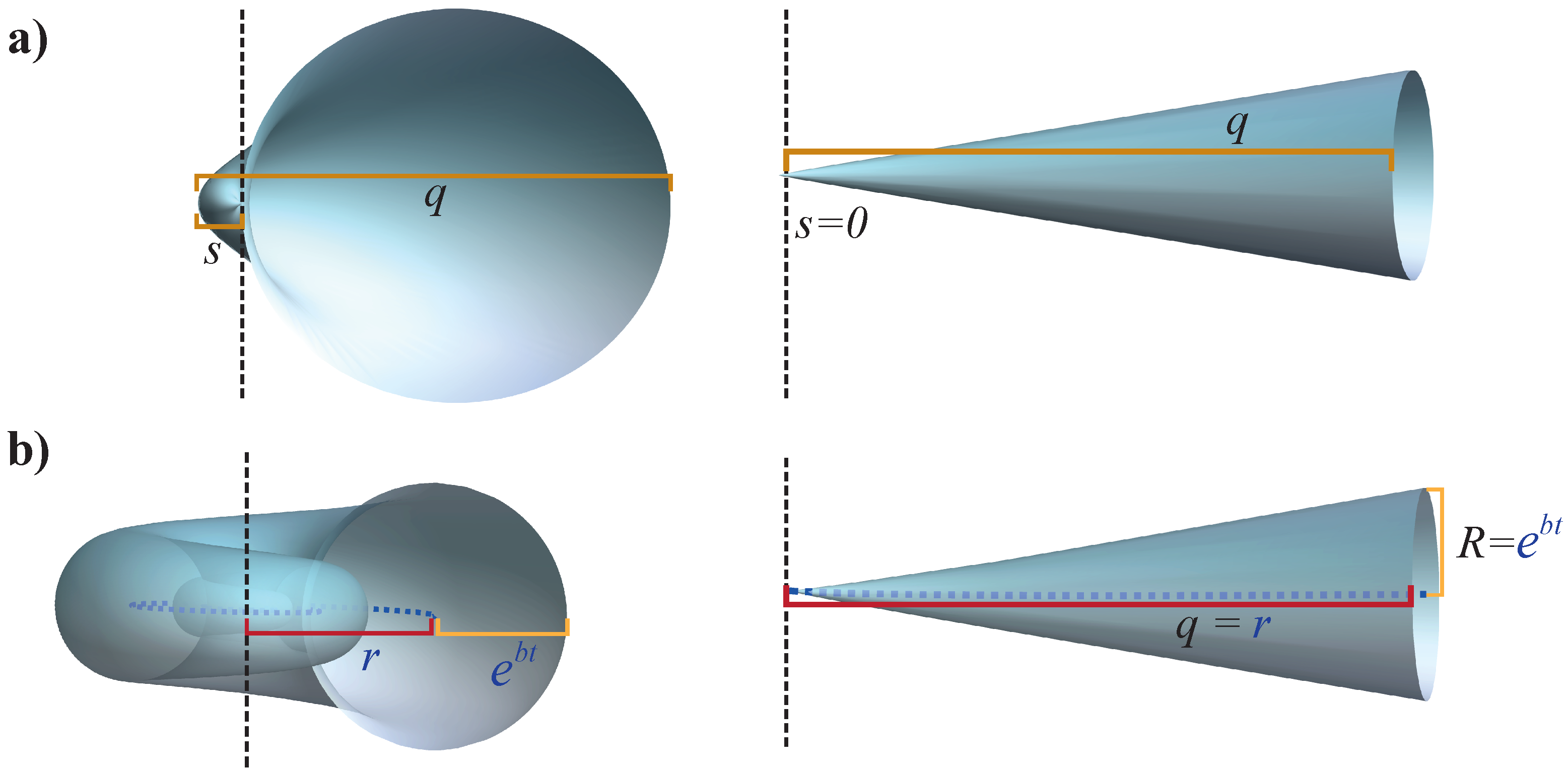
Orthoconic-like shells have straight and uncoiled morphologies which require specific considerations when measuring the values of the parameters. Although these shells are very different from common coiled shells, their forms can be reproduced with our model, with some considerations. In the model, for an uncoiled shell, ; therefore, parameter b should be measured as a planispiral or valve shell. However, because orthicone shells do not have whorls, that is, (Figure 3b,c), the equation for b now becomes . This can be interpreted as b having an infinite value, but it can be verified that is sufficient for generating conical shells. Considering parameter d, from the polar equation of the logarithmic spiral, we have ; therefore, as expected, for a large b, it becomes very small. However, by assuming that the larger possible value of the aperture radius is R, measured at the end of the cone (Figure 5b), then , where q is the length of the shell. The differences between the parameters b and d for the coiled and uncoiled shells are shown in Figure 5. Parameters a and can be calculated as shown in Figure 4d,e.

Figure 5.
Comparison of the measurements necessary to obtain (a) parameter b and (b) parameter d in coiled and uncoiled shells.
2.6. Some Additional Considerations about Measurements
The proposed parameters can be obtained through simple linear measurements, even physically on a specimen with a vernier. However, it is recommended that photographs of the specimens be used to achieve greater measurement precision as well as to facilitate parameter calculation and plotting. Correct alignment of the digitalized shell was established using the methodology of Callomon [49] for apertural, lateral, and apical views.
Our model and measurement methods were implemented in Wolfram Mathematica software [50] to automatically calculate the coiling axes, distances, vectors, and values of six parameters (b, d, z, a, and ). The required inputs are the coordinates of specific points on the shell. Using linear algebra methods, the distances and angles shown in Figure 3 and Figure 4 were obtained, and a 3D reconstruction of the specimen model is displayed. A Mathematica Notebook containing the functions for the mathematical model, graphic representations, and the proposed measurement procedure on digital images of real specimens is freely available at https://github.com/jlaragonvera/Mathematica-Notebooks (accessed on 8 March 2023).
2.7. Extra Parameters
As we are interested in building a practical theoretical morphospace, having few parameters is important. In this study, we considered the six described parameters () for modeling and generating morphospaces; however, the mathematical structure of the model can be modified to include additional parameters. As a demonstration, three additional parameters related to the ornamentation of the shell and displacement of the aperture with respect to the coiling axis are described. The purpose of this subsection is to show how the geometrical model can be modified and improved to simulate some specific morphological characteristics of the shells.
2.7.1. Ornamentation of the Generating Curve
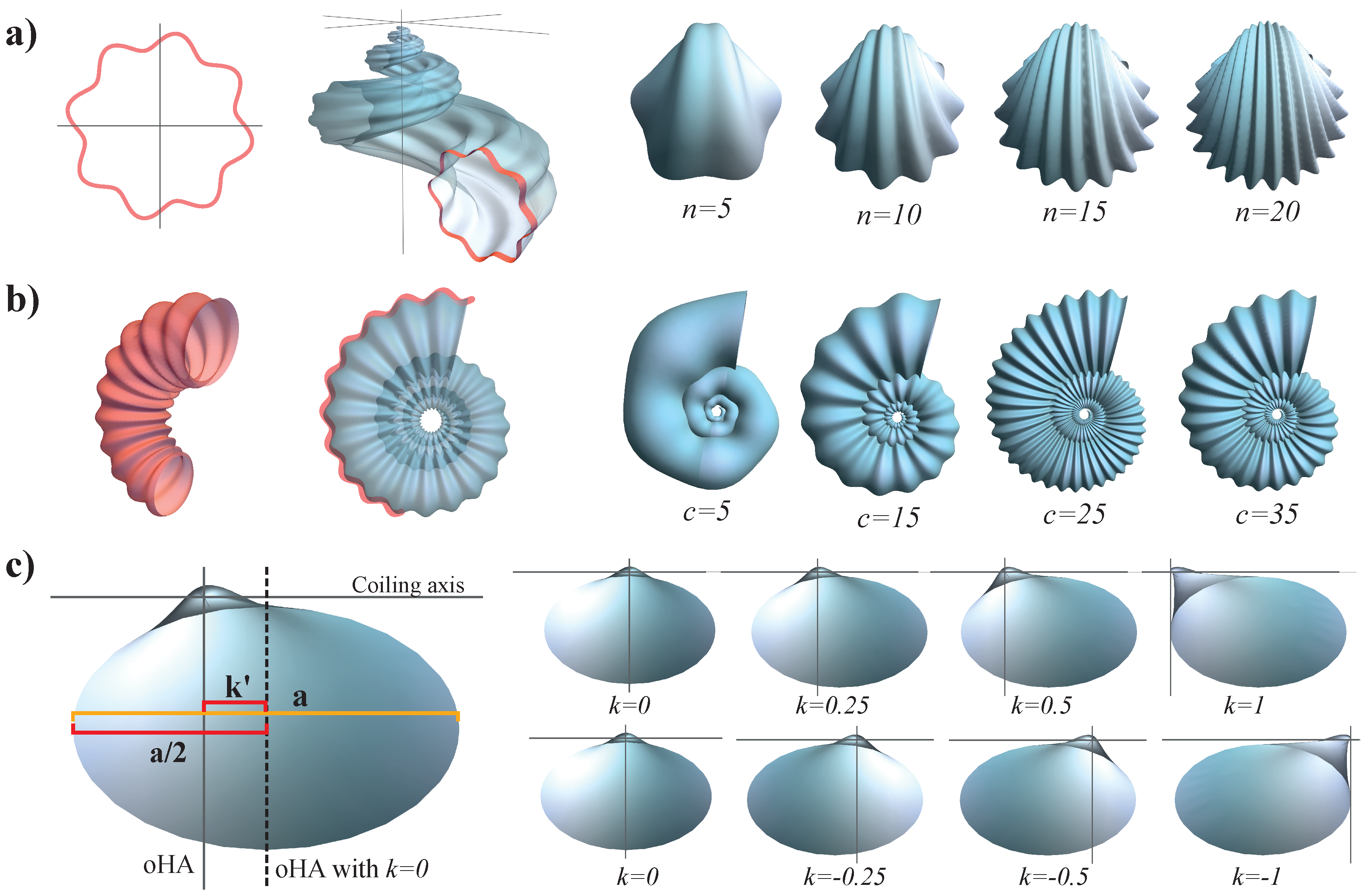
A parameter n can be used to produce ornamentation along the generating curve, given by the senoidal function: , where n is the number of peaks of the sin function (Figure 6a). The parametric equation of the generating curve with this modification is:

Figure 6.
Graphic representation of the additional parameters: (a) parameter n (oscillation in the generating curve), (b) parameter c (oscillation in the radio of the generating curve), and (c) parameter k (displacement of the aperture). In addition, examples of shell modification when the parameter values change are presented. In (c), represents the orthogonal hinge axis.
The reference value n= can be adjusted to model the amplitude of the wave and determine the corrugation depth. This parameter can be applied to any shell morphology; however, it is more commonly used in bivalve ornamentation.
2.7.2. Oscillating Radius of the Generating Curve
An ornamentation similar to ribs resulting from an oscillatory change in the radius of the generating curve can be introduced by means of a parameter c as the frequency of a sin function which depends on whorl number t. This produces corrugation along the shell surface (Figure 6b), and the equation of the generating curve becomes
The value of c represents the number of peaks and valleys in half a turn. The reference value can be adjusted to increase or decrease the depth of the ribs.
2.7.3. Displacement of the Aperture
The displacement of the aperture along the direction of the coiling axis, which is commonly observed in bivalves, can be reproduced by adding k units along the binormal in the generating curve equation:
Theoretically, the orthogonal hinge axis of the bivalves is located at the middle of the aperture when . It is necessary to specify the sign of k as positive when the right valve is measured, and negative for the left valve. Figure 6c shows the measurements and the proportions required to obtain k for the bivalve specimens. If is the distance between the orthogonal hinge axis when and the orthogonal hinge axis of the specimen, then .
3. Results
3.1. Theoretical Morphospaces
The model parameters constitute the axes of a six-dimensional space; the systematic variations in the values of the six parameters are visualized in a theoretical morphospace where all shell forms, within the established range values, are represented. For visualization purposes, adequate combinations of parameters were selected to generate two-dimensional and three-dimensional morphospaces, where the most remarkable morphological changes in our model can be appreciated.
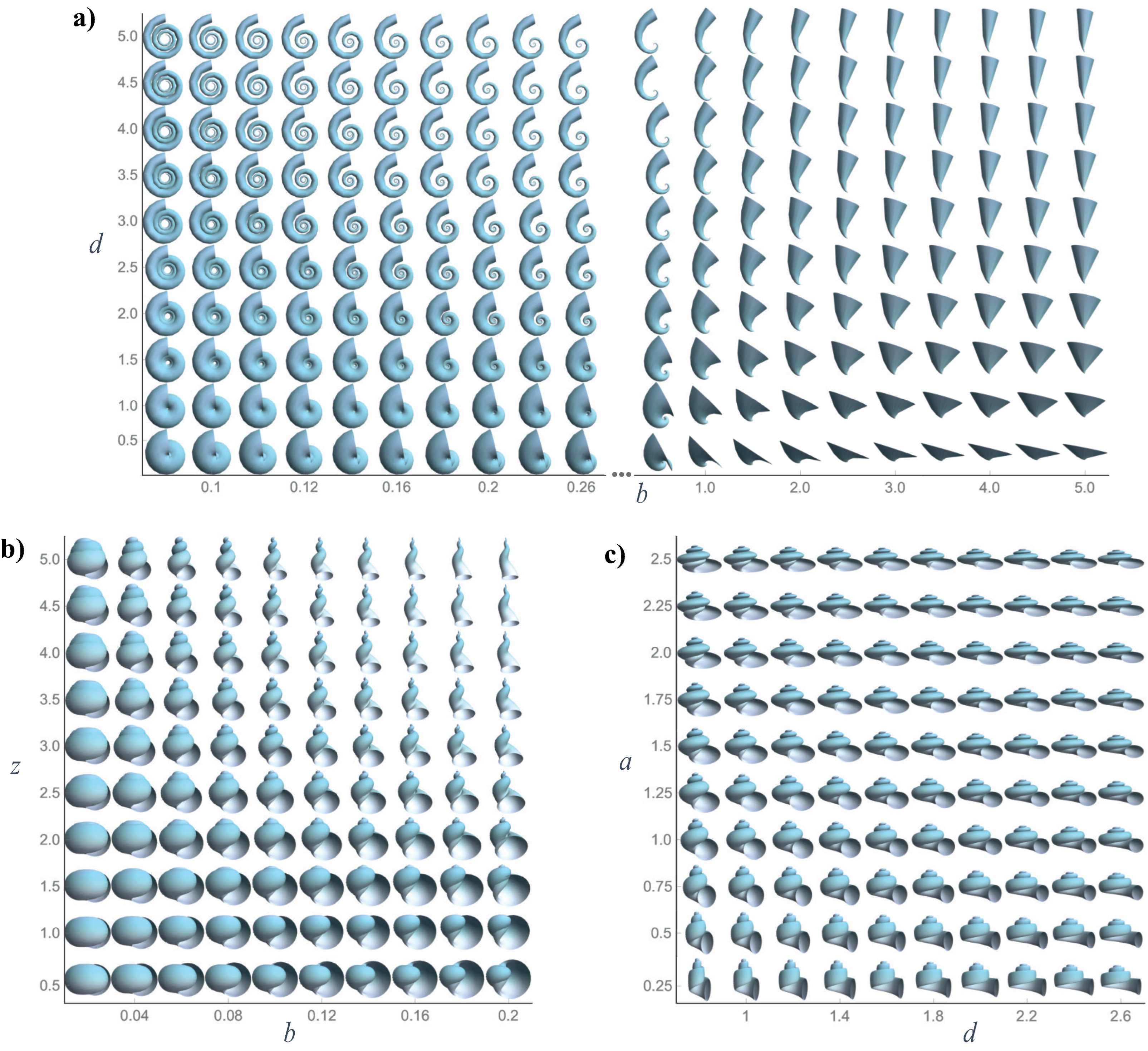
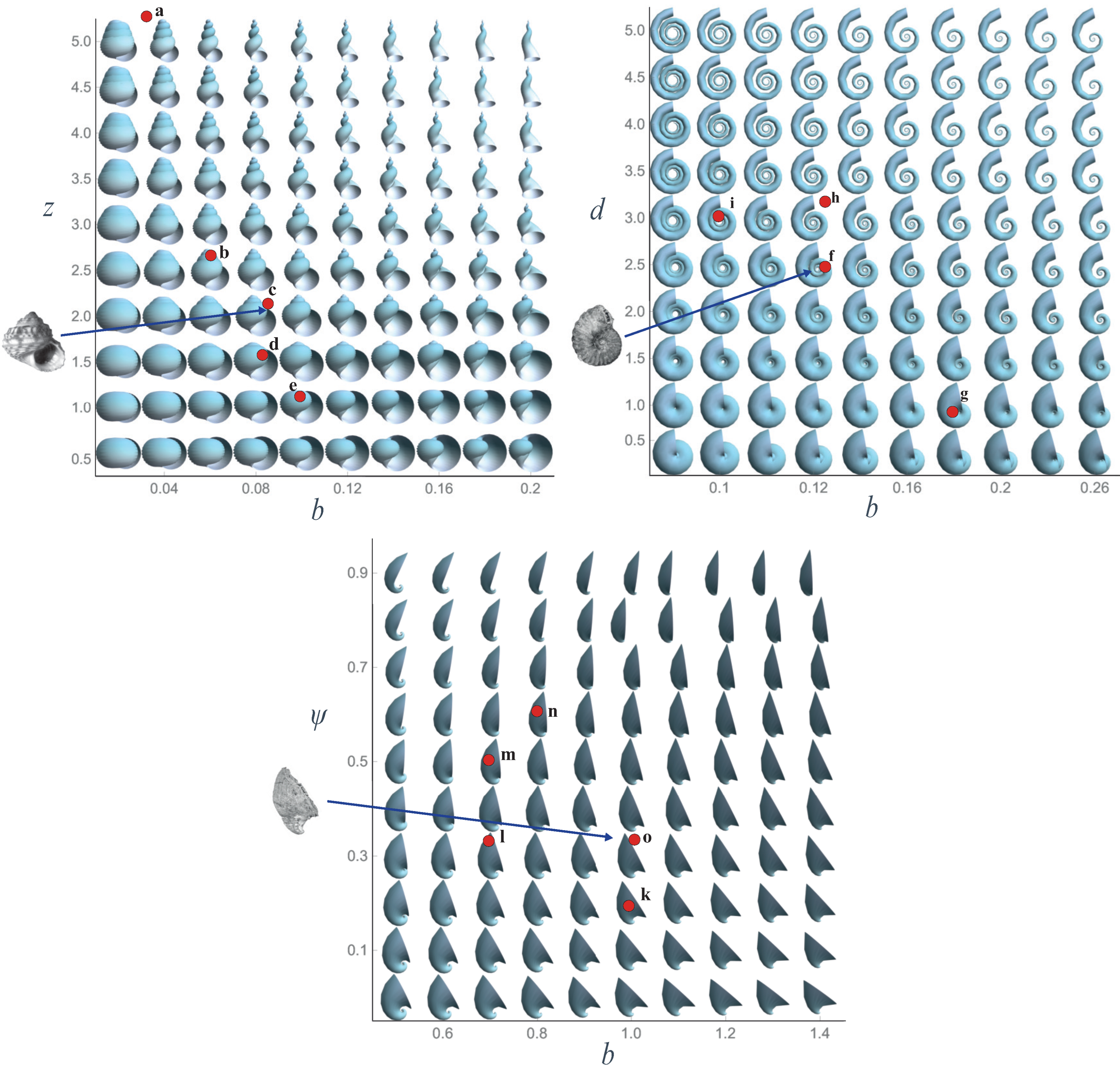
In Figure 7a, the theoretical morphospace for the planispiral shells in apical view is shown. As parameter b accounts for the whorl expansion rate, the larger its value, the more open the shells. Uncoiled shells (orthocone-like shells) can be modeled with higher values of b () because the expansion rate increases rapidly in a single whorl in which the shell cannot be coiled. Parameter d can reach when dealing with helicoidal shells; however, when working with planispiral shells, d values less than 1 interfere with coiling in the same plane. In orthoconic shapes, an increase in d lengthened the shell. The two-dimensional morphospace defined by parameters b and z reconstructs the helicoidal shell morphologies, being only planispiral when ; on the other hand, the higher the value of parameter z, the greater the displacement along the coiling axis (Figure 7b).The variation a in the shape of the aperture from elongated to widened is presented in Figure 7. The value of parameter a is systematically varied with the values of parameter d and it is observed that the 2D morphospace is filled with all possible shells formed by the combination of these two parameters.

Figure 7.
Two-dimensional theoretical morphospaces: (a) , with parameter values , , , and ; (b) , with parameter values , , , and ; and (c) , with parameter values , , , and .
Figure 8 shows the theoretical morphospace constructed by varying the three model parameters that define the form of the logarithmic spiral (2), that is, . These parameters lead to the most obvious overall variations in the shell morphology, as they control the whorl expansion growth and horizontal and vertical displacements, respectively. By varying these three parameters, different shell shapes can be reproduced, such as planispiral (e.g., ammonoids), helicoidal (e.g., gastropods), orthoconic (e.g., belemnites and rudists), and gyroconic (e.g., heteromorphic ammonoids).
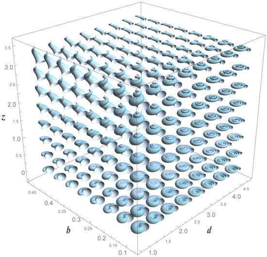
Figure 8.
There-dimensional theoretical morphospace with parameter values , , and . Only the forms belonging to the frontal faces of the cube are shown for better representation.
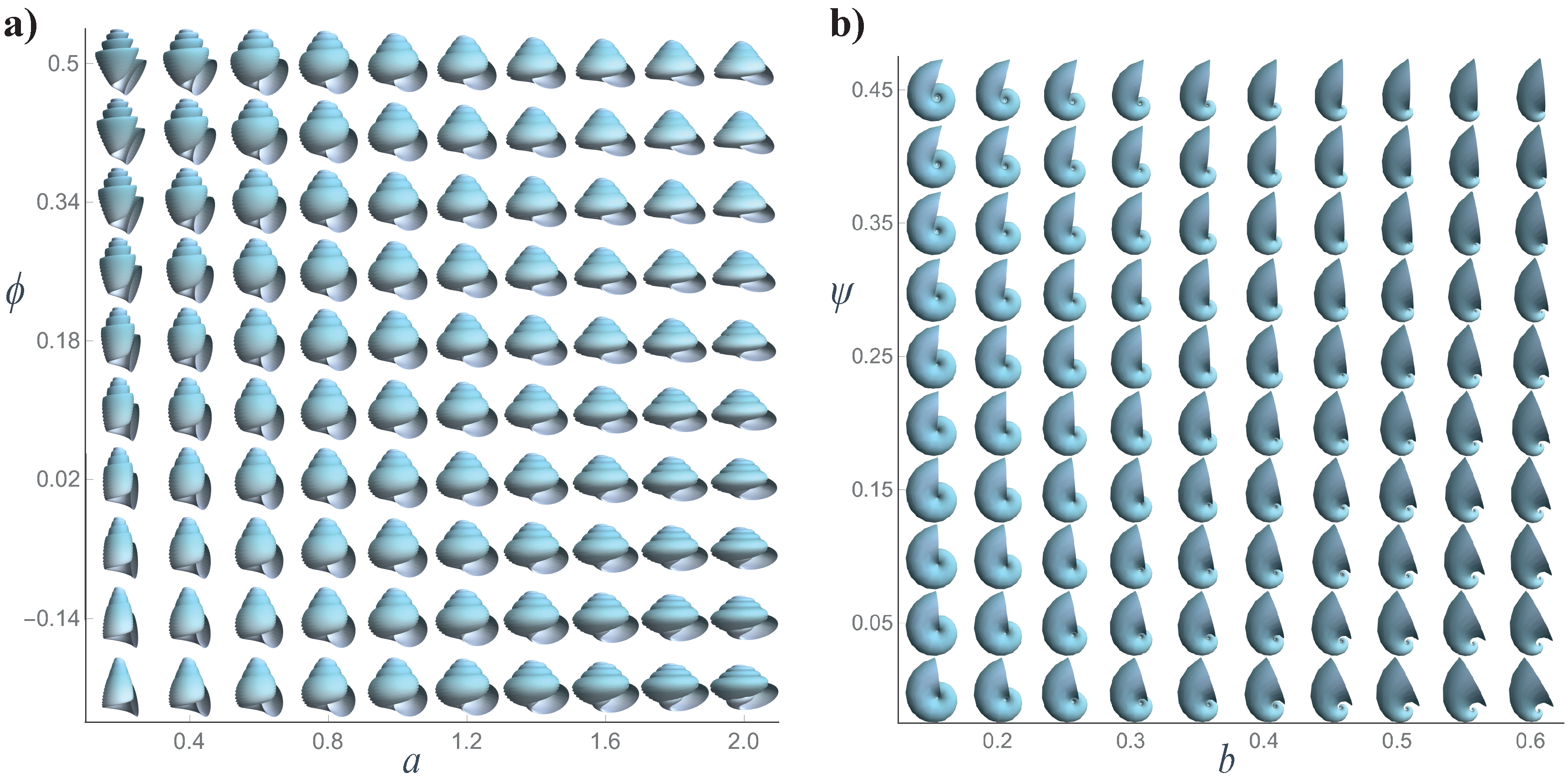
In Figure 9, we show morphospaces related to angular changes in the generating curve of the model, that is, the shell aperture. The apertural view of the simulated shells allows observation of the rotation of the aperture, as well as ellipsoidal changes, going through narrow (), circular (), and wide () aperture shells (Figure 9a). Although the values of b, d, and z are the same, this morphospace shows that the final shell morphology varied significantly with the form and orientation of the aperture with respect to the coiling axis. The rotation of the aperture carried out by parameter is required to model valve-like shells. Its variation is observable in the lateral view of the shell, and Figure 9b shows the two-dimensional morphospace .

Figure 9.
Two-dimensional theoretical morphospaces: (a) , with parameter values , , , and ; and (b) , with parameter values , , , and .
3.2. Application Example: Fossil Shells
Once the theoretical morphospaces were constructed, the next crucial step was to obtain the values of the parameters by measuring them in the actual shells. For this purpose, we used photographs of the fossil specimens described in Section 2.1.
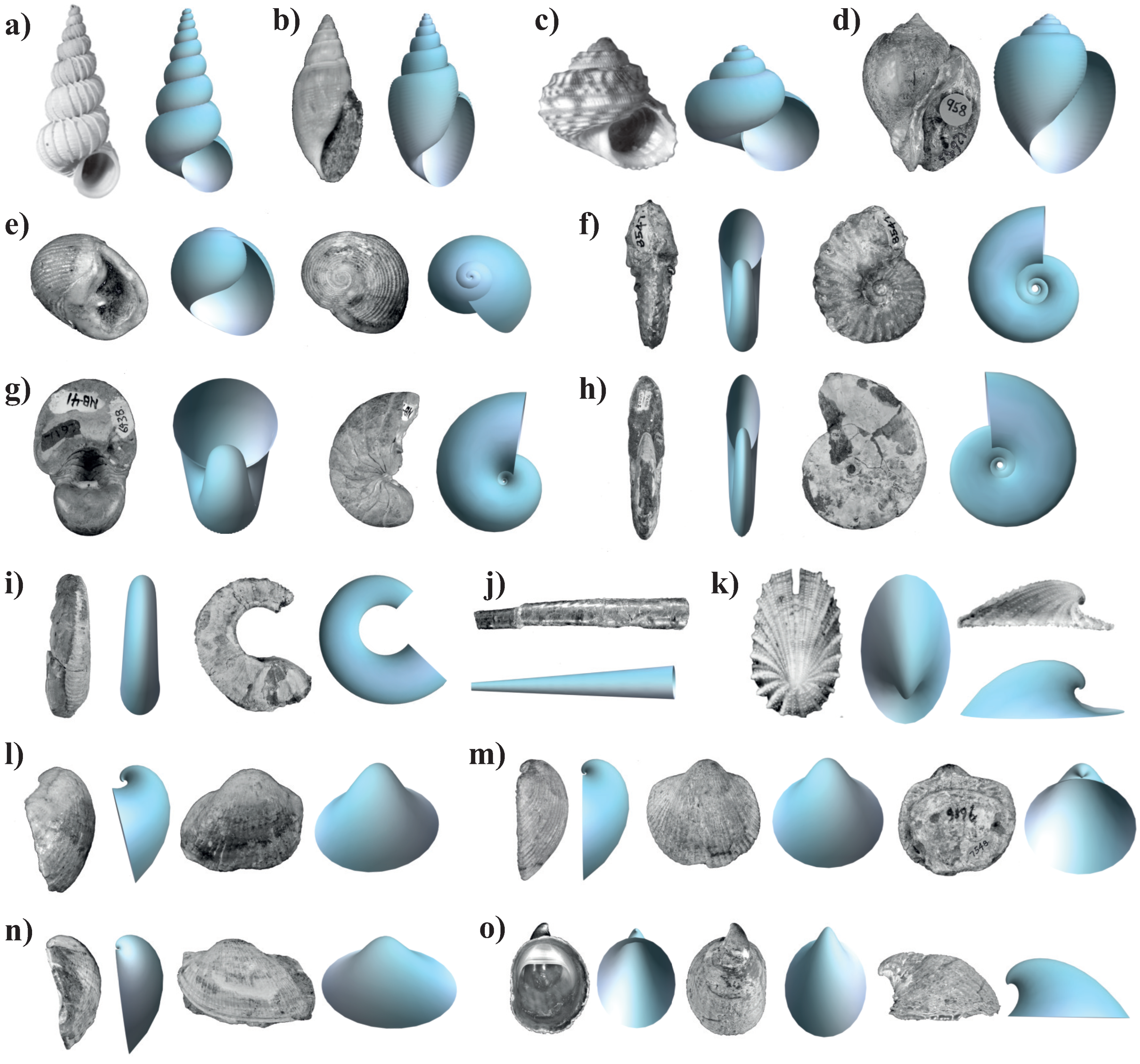
Table 1 shows the values of the six parameters obtained from the photographs of the fossil specimens according to the procedures described in Section 2.4. With these values, the theoretical models were generated and comparisons with real specimens are presented in Figure 10, which shows that, in general, the theoretical model offers adequate representations of the real shell. Parameters b, d, and z account for the general form of the shell, whereas parameters a, , and control the aperture shape.

Table 1.
Measured parameter values of the specimens studied in this work. NA indicates that these measurements could not be obtained due to the preservation of the specimen.

Figure 10.
The studied specimens and their respective shapes obtained with the mathematical model; the length of the shell specimen is indicated in parenthesis: (a) Asperiscala pacis (10 mm); (b) Acteon sullivanae (8 mm); (c) Lirularia pedroana (5 mm); (d) Brachysphingus mammilatus (35 mm); (e) Biplica obliqua (15 mm); (f) Oregoniceras siskiyouense (30 mm); (g) Nautilus aff. N. cookanum (40 mm); (h) Cleoniceras (Grycia) susukii (100 mm); (i) Shasticrioceras patricki (50 mm); (j) Baculites boulei (70 mm); (k) Scelidotoma bella (5 mm); (l) Cucullaea morani (20 mm); (m) Glycymerita banosensis (40 mm); (n) Indogrammatodon vancouverensis (20 mm); and (o) Crepidula adunca (7 mm).
Parameter a is a morphological generalization which is applicable to all types of shells when the aperture can be approximated as an ellipse, and the parameters and produce a particular orientation which is more relevant only for some morphologies.
From Table 1, we notice that parameters b, d, and a can be measured for all specimens. Specimens have helicoidal coiling only when , which corresponds to shells of the Gastropoda class. The higher the value of z, the more vertical the displacement; for instance, Asperiscala pacis (Figure 10a) had the highest z value, whereas Sinum scopulosum and Biplica obliqua had the lowest vertical displacement (Figure 10d,e).
Scelidotoma bella and Crepidula adunca also belong to the Gastropoda class; however, because of their limpet morphology, they were measured using a valve-like shell methodology (Figure 10k,o). These types of shells, such as bivalves and limpets, are distinguished by high values of b (), , and . It should be noted that is important for valve-like specimens, which enables the development of apertures with positions aligned with the umbo in the apical view (Figure 10l–n). Indeed, can only be measured in a specimen with a complete aperture visible in apical-view photographs. This type of photograph is not often taken for helicoidal specimens; however, an example of the measurement of in a helicoidal shell is presented in Figure 10e. In the case of the Cephalopoda class, measuring is difficult because of the lack of preservation of aperture inclination.
The cephalopod specimens corresponded to planispiral shells () without an inclination in the aperture (). Two heteromorph ammonoids, Shasticrioceras patricki and Baculites boulei, were selected to demonstrate the potential of the theoretical model for generating shells with different coilings. The first shows incomplete coiling and the second represents an uncoiled shell. Baculites boulei can be modeled when parameter b tends to infinity; however, a value of makes the shell coiling negligible. Parameters d and a account for the proportions of the length and width of the orthocone shell, respectively.
The next step in the theoretical morphospace analysis is to plot the position of the measured specimens in the proposed theoretical morphospaces, as shown in Figure 11. The final and perhaps the most difficult step of a theoretical morphospace analysis is to analyze the functional significance of both existing and non-existing forms in the morphospace [7]. For this, a large collection of specimens is required and will be the purpose of a future publication. The aim of the present study was to propose an adequate model for theoretical morphospace analysis and test it using representative samples.
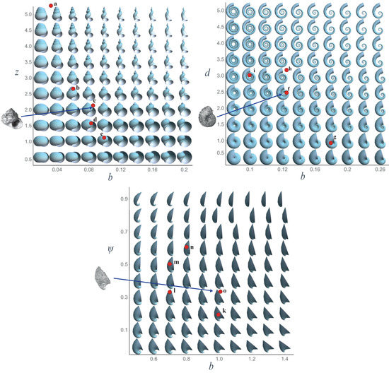
Figure 11.
The studied specimens mapped on the generated theoretical morphospaces. Each point represents a specimen of helicoidal, planispiral, or bivalve-like shells. Morphologies are identified with the same letter as in Figure 10.
4. Discussion
In this study, we propose a mathematical model based on parametric surfaces and a theoretical morphospace for different classes of mollusc shells. Different mathematical models were developed to describe mollusc shells, and all of them made particular contributions towards a comprehensive study of shell geometry. The application of both fixed (coiling axis) and moving (Frenet frame) reference systems has been proposed in other works to generate an appropriate representation of the shell ([40,41,42]). However, the contribution of the theoretical model proposed here is its ability to be used in empirical studies, owing to the standardized methodology for estimating the parameter values for different forms of real specimens, which is a missing part in the model of [40,41]. This contribution is accompanied by the visualization of theoretical morphospaces where the specimens can be mapped once their theoretical parameters are calculated.
Our model rests on the logarithmic spiral equation, which has well-known self-similarity properties. The natural ontogenetic growth of the shell, however, usually deviates from the self-similarity property of the spiral. Nevertheless, this geometric property not only facilitates the modeling of the shell and the definition of the parameters but also yields an algebraic dependence between some parameters when the equations are reviewed. For instance, the parameter b influences the linear parameters d and z, which are elements of the logarithmic spiral. The horizontal displacement d is influenced by parameter a when it is measured in the specimens, because the ellipse is given by the rate of the horizontal proportion in relation to the vertical axis of the ellipse. However, systematic variation in the parameter values does not affect the process of measurement, shell modeling, or theoretical morphospace construction (see Figure 7c). Following the idea of Gerber [51] regarding the geometry of morphospaces, there is no algebraic dependency among parameters when the morphospace is generated. This is because all parameters can be varied freely and independently, thereby modeling theoretical shells that fill the six dimensions of the theoretical morphospace.
The model proposed in this study does not simulate shell morphogenesis as in other models ([15,32,33,35]). In general, the mechanisms of shell morphogenesis remain poorly understood; however, the geometrical model and parameters proposed here could be useful tools to support developmental studies in mollusc shells (e.g., Johnson et al. [52] and their relationship with Raup’s parameters).
An advantage of our model is its ease of estimating theoretical parameter values in shell specimens, which has proven to be an advantage in empirical work (e.g., the success of Raup’s model for data acquisition and its application in subsequent works). In the field of theoretical morphology, estimating model parameters from measurements in a real shell is a crucial step. In this regard, George R. McGhee wrote: "if your parameters are too abstract and unobtainable from actual biological form, then you must return to Step One and start over again with a different model’ (McGhee [7]). In this study, we propose a simple methodology to obtain the model parameters from measurements in real shells. This methodology rests on distinguishing the coiling axis as an important component for localizing the measured distances. Some authors consider that the coiling axis is an imaginary axis without biological meaning ([29,30,31]); however, we consider it a useful component when the shell is modeled using initially a fixed coordinate system, as in the proposed model, which helps to orient the shell photographs and standardize the measurement in the specimens. An advantage of the self-similarity of the logarithmic spiral is that it allows us to obtain the values of the parameters at any given whorl. Therefore, it is possible to measure incomplete or fragmented specimens, which are common in paleontological studies.
The model and morphospace developed here are feasible alternatives for future studies on the morphological characterization of mollusc shells. Although the six proposed parameters define a six-dimensional theoretical morphospace which cannot be visualized, the morphological parameters of interest for a specific study can be selected and represented using different morphospace configurations with lower dimensions. Some parameters are more suitable with certain shell morphologies; for instance, the tilting by parameter better describes valve-like shells, and parameter z is essential to model helicoidal forms. It should be noted that the model focused on characterizing the general form of mollusc shells; however, the mathematical structure of the model allows the modification or addition of new parameters to make the reconstruction of the shell more detailed. In this context, the aperture form considerably influences the general shell morphology. Usually, the form differs significantly from that of an ellipse. The proposed model can be modified to specify a new equation for the generating curve which is more realistic for a specific type of aperture. Additionally, new parameters related to the ornamentation of the shell and the displacement of the aperture with respect to the coiling axis can be included if the measured shell group requires them.
In summary, the theoretical model proposed here constitutes a useful tool for constructing a practical theoretical morphospace for the morphological analysis of mollusc shells. Contrary to others models that also employ a fixed coordinate system and a moving Frenet frame, a simple method for obtaining the mathematical parameter from photographs of real specimens is proposed. The model focuses on shells with self-similar growth in the radius of the spiral and aperture, which simplifies the measurement of the parameters in the shell specimens. DUe to the incommensurability and range values of these parameters, the theoretical morphospace must be analyzed as an affine space (Huttegger and Mitteroecker [53]), and the implementation of other measures, such as Mahalanobis distances, is required. The mathematical structure of the model allows for the modification or addition of new parameters, if a specific morphological study is required. The proposed methodology is adequate for obtaining the theoretical parameters and coiling axis of the shell using simple linear and angular measurements on the apertural and apical views of the specimens. It should be emphasized that the same model can analyze different morphologies from the principal classes of Mollusca (Gastropoda, Cephalopoda, and Bivalvia), which include helicoidal, planispiral, conic, and valve-like shells. These classes are important and diverse groups throughout the geological time up to the present day; therefore, the proposed theoretical morphospace can be applied to paleontological or biological studies concerned with the quantitative characterization or disparity analysis of mollusc shells.
Author Contributions
Conceptualization, J.L.A.; methodology, J.L.A. and G.C.-F.; software, G.C.-F.; validation, G.C.-F. and J.L.A.; formal analysis, G.C.-F.; investigation, G.C.-F.; resources, J.L.A.; data curation, G.C.-F.; writing—original draft preparation, G.C.-F.; writing—review and editing, J.L.A. and G.C.-F.; visualization, G.C.-F.; supervision, J.L.A.; project administration, J.L.A.; funding acquisition, J.L.A. All authors have read and agreed to the published version of the manuscript.
Funding
Gabriela Contreras-Figueroa received fellowship 595922 from CONACYT.
Institutional Review Board Statement
Not applicable.
Data Availability Statement
Wolfram Mathematica Notebooks with functions to generate the mathematical model for graphic representations and for the measurement procedure in digital images of real specimens is freely available at https://github.com/jlaragonvera/Mathematica-Notebooks (accessed on 8 March 2023).
Acknowledgments
Gabriela Contreras-Figueroa is a doctoral student from Programa de Doctorado en Ciencias Biomédicas, Universidad Nacional Autónoma de México (UNAM) and received fellowship 595922 from CONACYT. She also wishes to thank the National History Museum of Los Angeles County for awarding her the Student Collections Study Award and Austin Hendy for his guidance through the collection, many discussions, and suggestions.
Conflicts of Interest
The authors declare no conflict of interest.
References
- Thompson, D.W. On Growth and Form; Cambridge University Press: London, UK, 1917. [Google Scholar]
- Moseley, H. On the Geometrical Forms of Turbinated and Discoid Shells. Philos. Trans. R. Soc. Lond. 1838, 128, 351–370. [Google Scholar]
- Porges, K.; Stewart, I.G.; Hoßfeld, U.; Levit, G.S. From Idea to Law: Theory, Concept and Terminological Formation in Ernst Haeckel’s Works. Russ. J. Dev. Biol. 2019, 50, 290–302. [Google Scholar] [CrossRef]
- Raup, D.M. The geometry of coiling in gastropods. Nat. Acad. Sci. Proc. 1961, 47, 602–609. [Google Scholar] [CrossRef] [PubMed]
- Raup, D.M. Computer as aid in describing form in gastropod shell. Science 1962, 138, 150–152. [Google Scholar] [CrossRef]
- Raup, D.M.; Michelson, A. Theoretical morphology of the coiled shell. Science 1965, 147, 1294–1295. [Google Scholar] [CrossRef]
- McGhee, G.R. The Geometry of Evolution; Cambridge University Press: New York, NY, USA, 2006. [Google Scholar]
- McGhee, G.R. Theoretical Morphology: The Concept and Its Applications; Columbia University Press: New York, NY, USA, 1999. [Google Scholar]
- Budd, G.E. Morphospace. Curr. Biol. 2021, 31, R1181–R1185. [Google Scholar] [CrossRef]
- Foote, M. The evolution of morphological diversity. Ann. Rev. Ecol. Syst. 1997, 28, 129–152. [Google Scholar] [CrossRef]
- Erwin, D.H. Disparity: Morphological pattern and development context. Palaentology 2007, 50, 57–73. [Google Scholar] [CrossRef]
- Dera, G.; Eble, G.J.; Neige, P.; David, B. The flourishing diversity of models in theoretical morphology: From current practices to future macroevolutionary and bioenvironmental challenges. Paleobiology 2008, 34, 301–317. [Google Scholar] [CrossRef]
- Johnston, M.R.; Tabachnick, R.E.; Bookstein, F.L. Landmark-Based Morphometrics of Spiral Accretionary Growth. Paleobiology 1991, 17, 19–36. [Google Scholar] [CrossRef]
- Savazzi, E. Biological aspects of theoretical shell morphology. Lethaia 1990, 23, 195–212. [Google Scholar] [CrossRef]
- Moulton, D.E.; Goriely, A.; Chirat, R. Mechanical growth and morphogenesis of seashells. J. Theor. Biol. 2012, 311, 69–79. [Google Scholar] [CrossRef] [PubMed]
- Haszprunar, G.; Wanninger, A. Molluscs. Curr. Biol. 2012, 22, R510–R514. [Google Scholar] [CrossRef] [PubMed]
- Stone, J.R. The Evolution of Ideas: A Phylogeny of Shell Models. Am. Nat. 1996, 148, 904–929. [Google Scholar] [CrossRef]
- Raup, D.M. Geometric analysis of shell coiling: General problems. J. Paleontol. 1966, 40, 1178–1190. [Google Scholar]
- Vermeij, G.J. Gastropod evolution and morphological diversity in relation to shell geometry. J. Zool. 1971, 163, 15–23. [Google Scholar] [CrossRef]
- Kohn, A.J.; Riggs, A.C. Morphometry of the Conus Shell. Syst. Zool. 1975, 24, 346–359. [Google Scholar] [CrossRef]
- Lovtrup, S.; Lovtrup, M. The Morphogenesis of Molluscan Shells: A Mathematical Account Using Bioogical Parameters. J. Morphol. 1988, 197, 53–62. [Google Scholar] [CrossRef]
- Cortie, M.B. Models for Mollusc Shell Shape. South Afr. J. Sci. 1989, 85, 454–460. [Google Scholar]
- McGhee, G.R. Shell Form in the Biconvex Articulate Brachiopoda: A Geometric Analysis. Paleobiology 1980, 6, 57–76. [Google Scholar] [CrossRef]
- Hutchinson, J.M. Control of gastropod shell shape; The role of the preceding whorl. J. Theor. Biol. 1989, 140, 431–444. [Google Scholar] [CrossRef]
- Stone, J.R. Cerioshell: A computer program designed to simulate variation in shell form. Paleobiology 1995, 21, 509–519. [Google Scholar] [CrossRef]
- Tursch, B. Spiral growth: The ’museum of all shells’ revisited. J. Molluscan Stud. 1997, 63, 547–554. [Google Scholar] [CrossRef]
- Swan, A.R.H. Heterochrony in helicoid spiral cones: A computer model for demonstrating heterochronic evolution. Palaeontol. Electron. 2015, 18, 1–11. [Google Scholar] [CrossRef] [PubMed]
- Okabe, T.; Yoshimura, J. Optimal designs of mollusk shells from bivalves to snails. Sci. Rep. 2017, 7, 42445. [Google Scholar] [CrossRef]
- Okamoto, T. Analysis of heteromorph ammonoids by differential geometry. Palaentology 1988, 31, 35–52. [Google Scholar]
- Ackerly, S.C. Kinematics of Accretionary Shell Growth, with Examples from Brachiopods and Molluscs. Paleobiology 1989, 15, 147–164. [Google Scholar] [CrossRef]
- Rice, S.H. The Bio-Geometry of Mollusc Shells. Paleobiology 1998, 24, 133–149. [Google Scholar] [CrossRef]
- Hammer, Ø.; Bucher, H. Models for the morphogenesis of the molluscan shell. Lethaia 2005, 38, 111–122. [Google Scholar] [CrossRef]
- Urdy, S.; Goudemand, N.; Bucher, H.; Chirat, R. Allometries and the morphogenesis of the molluscan shell: A quantitative and theoretical model. J. Exp. Zool. (Mol. Dev. Evol.) 2010, 314, 280–302. [Google Scholar] [CrossRef]
- Pappas, J.L.; Miller, D.J. A Generalized Approach to the Modeling and Analysis of 3D Surface Morphology in Organisms. PLoS ONE 2013, 8, e77551. [Google Scholar] [CrossRef] [PubMed]
- Chirat, R.; Goriely, A.; Moulton, D.E. The physical basis of mollusk shell chiral coiling. Proc. Natl. Acad. Sci. USA 2021, 118, e2109210118. [Google Scholar] [CrossRef] [PubMed]
- Shimizu, K.; Iijima, M.; Setiamarga, D.H.; Sarashina, I.; Kudoh, T.; Asami, T.; Gittenberger, E.; Endo, K. Left-right asymmetric expression of dpp in the mantle of gastropods correlates with asymmetric shell coiling. EvoDevo 2013, 4, 15. [Google Scholar] [CrossRef] [PubMed]
- Noshita, K. Quantification and geometric analysis of coiling patterns in gastropod shells based on 3D and 2D image data. J. Theor. Biol. 2014, 363, 93–104. [Google Scholar] [CrossRef]
- Noshita, K.; Shimizu, K.; Sasaki, T. Geometric analysis and estimation of the growth rate gradient on gastropod shells. J. Theor. Biol. 2016, 389, 11–19. [Google Scholar] [CrossRef]
- Liew, T.S.; Schilthuizen, M. A Method for Quantifying, Visualising, and Analysing Gastropod Shell Form. PLoS ONE 2016, 11, e0157069. [Google Scholar] [CrossRef]
- Illert, C. Formulation and Solution of the Classical Seashell Problem. Nuovo C. 1989, 11, 761–780. [Google Scholar] [CrossRef]
- Fowler, D.R.; Meinhardt, H.; Prusinkiewicz, P. Modeling seashells. Comput. Graph. (ACM) 1992, 26, 379–387. [Google Scholar] [CrossRef]
- Prusinkiewicz, P.; Fowler, D.R. Shell models in three dimensions. In The Algorithmic Beauty of Sea Shells; Springer: Berlin/Heidelberg, Germany, 2009; pp. 166–185. [Google Scholar]
- Ashline, G.L.; Ellis-Monaghan, J.A.; Kadas, Z.M.; McCabe, D.J. Modeling Seashell Morphology. In UMAP/ILAP Modules: Tools for Teaching; COMAP: Bedford, MA, USA, 2009; pp. 101–139. [Google Scholar]
- Gray, A.; Abbena, E.; Salamon, S. Modern Differential Geometry of Curves and Surfaces with Mathematica, 3rd ed.; Chapman & Hall/CRC: Boca Raton, FL, USA, 2006. [Google Scholar]
- Vermeij, G.J. A Natural History of Shells; Princeton University Press: Princeton, NJ, USA, 1995. [Google Scholar]
- Edie, S.M.; Collins, K.S.; Jablonski, D. Specimen alignment with limited point-based homology: 3D morphometrics of disparate bivalve shells (Mollusca: Bivalvia). PeerJ 2022, 10, e13617. [Google Scholar] [CrossRef]
- Carter, J.G.; Harries, P.; Malchus, N.; Sartori, A.; Anderson, L.; Bieler, R.; Bogan, A.; Coan, E.; Cope, J.; Cragg, S.; et al. Treatise Online no. 48: Part N, Revised: Illustrated Glossary of the Bivalvia. Treatise Online 2012, 1. [Google Scholar]
- Cox, L.R.; Nutall, C.P.; Trueman, E. General Features of bivalva. In Treatise on Invertebrate Paleontology. Part N, Mollusca 6, Bivalvia; Moore, R.C., Ed.; CO & Lawrence, Geological Society of America & University of Kansas: Lawrence, KS, USA, 1969; Volume 1, pp. 1–129. [Google Scholar]
- Callomon, P. Standard Views for Imaging Mollusk Shells; American Malacological Society: Tuscaloosa, AL, USA, 2019; pp. 1–19. [Google Scholar]
- Wolfram Inc. Mathematica, Version 13.2; Wolfram Inc.: Champaign, IL, USA, 2022. [Google Scholar]
- Gerber, S. The geometry of morphospaces: Lessons from the classic Raup shell coiling model. Biol. Rev. 2017, 92, 1142–1155. [Google Scholar] [CrossRef]
- Johnson, A.B.; Fogel, N.S.; Lambert, J.D. Growth and morphogenesis of the gastropod shell. Proc. Natl. Acad. Sci. USA 2019, 116, 6878–6883. [Google Scholar] [CrossRef] [PubMed]
- Huttegger, S.M.; Mitteroecker, P. Invariance and Meaningfulness in Phenotype Spaces. Evol. Biol. 2011, 38, 335–351. [Google Scholar] [CrossRef]
Disclaimer/Publisher’s Note: The statements, opinions and data contained in all publications are solely those of the individual author(s) and contributor(s) and not of MDPI and/or the editor(s). MDPI and/or the editor(s) disclaim responsibility for any injury to people or property resulting from any ideas, methods, instructions or products referred to in the content. |
© 2023 by the authors. Licensee MDPI, Basel, Switzerland. This article is an open access article distributed under the terms and conditions of the Creative Commons Attribution (CC BY) license (https://creativecommons.org/licenses/by/4.0/).

