Article

Environmental Drivers of Amphibian Breeding Phenology across Multiple Sites

by
Michael F. Benard
1,* and
Katherine R. Greenwald
2,*
1
Department of Biology, Case Western Reserve University, Cleveland, OH 44106, USA
2
Department of Biology, Eastern Michigan University, Ypsilanti, MI 48197, USA
*
Authors to whom correspondence should be addressed.
Diversity 2023, 15(2), 253; https://doi.org/10.3390/d15020253
Submission received: 4 October 2022 / Revised: 2 February 2023 / Accepted: 6 February 2023 / Published: 10 February 2023
(This article belongs to the Special Issue Amphibian Ecology in Geographically Isolated Wetlands)

Abstract

:
A mechanistic understanding of phenology, the seasonal timing of life history events, is important for understanding species’ interactions and the potential responses of ecological communities to a rapidly changing climate. We present analysis of a seven-year dataset on the breeding phenology of wood frogs (Rana sylvatica), tiger salamanders (Ambystoma tigrinum), blue-spotted salamanders (Ambystoma laterale), and associated unisexual Ambystoma salamanders from six wetlands in Southeast Michigan, USA. We assess whether the ordinal date of breeding migrations varies among species, sexes, and individual wetlands, and we describe the specific environmental conditions associated with breeding migrations for each species/sex. Breeding date was significantly affected by species/sex identity, year, wetland, and the interactions between species/sex and year as well as wetland and year. There was a great deal of variation among years, with breeding occurring nearly synchronously among groups in some years but widely spaced between groups in other years. Specific environmental triggers for movement varied for each species and sex and changed as the breeding season progressed. In general, salamanders responded to longer temperature lags (more warmer days in a row) than wood frogs, whereas wood frogs required longer precipitation lags (more rainy days in a row) than salamanders. Wood frogs were more likely to migrate around the time of a new moon, whereas in contrast, Ambystoma salamander migration was not associated with a moon phase. Ordinal day was an important factor in all models, suggesting that these amphibians require a latency period or similar mechanism to avoid breeding too early in the year, even when weather conditions appear favorable. Male wood frogs migrated earlier than female wood frogs, and male blue-spotted salamanders migrated earlier than female A. laterale and associated unisexual females. Larger unisexual salamanders migrated earlier than smaller individuals. Differences in species’ responses to environmental cues led to wood frogs and A. laterale breeding later than tiger salamanders in colder years but not in warmer years. This suggests that, as the climate warms, wood frog and A. laterale larvae may experience less predation from tiger salamander larvae due to reduced size differences when they breed simultaneously. Our study is one of few to describe the proximate drivers of amphibian breeding migrations across multiple species, wetlands, and years, and it can inform models predicting how climate change may shift ecological interactions among pond-breeding amphibian species.

1. Introduction

Variation in phenology, i.e., the seasonal timing of life history events, can have important effects on an organism’s survival, growth, and interactions with other species [1,2,3]. For example, early spring budburst increases the risk of frost damage in plants [4], earlier emergence from hibernation can increase growth in rodents [5], and differences in relative breeding dates can alter predator-prey interactions between aquatic dragonflies and amphibian larvae [6]. Year-to-year variation in phenology is driven by variation in environmental factors, such as precipitation, temperature, and photoperiod, which trigger when life history events occur. The specific combination of environmental cues varies not only among species [7], but it can also vary between sexes of the same species [8] and across small spatial scales [9]. Understanding the environmental variables that drive differences in phenology between species, sexes, and populations is increasingly important in the face of global climate change. As temperatures rise and patterns of precipitation change, the phenology of many organisms is changing [10,11]. In some groups, particularly some plants and insects, the cues responsible for phenology have been identified in enough detail to develop predictive models of how the phenology of these organisms is expected to shift in a changing world [12,13,14]. Identifying the environmental cues responsible for organisms’ phenology can play a key role in determining how climate change is likely to generate phenological variation among species, sexes, and populations, which in turn can provide insights into how this may affect individual populations and ecological communities.
Amphibians are an important group in which to understand the links between environmental cues and phenology. Variation in breeding phenology is ecologically significant; for example, it affects larval development rates [15,16] and the outcome of interspecific interactions [6,17,18]. The seasonal timing of amphibian breeding exhibits some of the strongest shifts in phenology due to climate change, but there is also substantial variation among species in the strength of phenological shifts, ranging from species with large changes in breeding date to other species with no change [11]. Multiple studies found correlations between changes in average breeding date and changes in average seasonal temperature and precipitation [7,19,20,21]. However, in addition to testing for correlations between seasonal average weather and breeding date, there is also value in identifying the specific environmental triggers that lead to breeding activity. Although such mechanistic models of breeding activity are increasingly common in plants and some animals [12,14], they are much less commonly applied to amphibians [22,23,24].
Four factors have been identified as having important roles in the timing of amphibian breeding migrations: temperature, precipitation, lunar phase, and a latency period. Temperature and precipitation are often considered in models in different ways and are often constrained by the type of data available. For example, a four-year study of mole salamander (Ambystoma talpoideum) immigration considered multiple temperature (e.g., maximum air temperature, minimum air temperature, air temperature range) and precipitation (e.g., daily precipitation and water level in wetlands) metrics and found the best models for adult breeding immigration varied between sites but often included minimum temperature and water level [23]. Regardless of how they are incorporated into models, both temperature and precipitation are important triggers for breeding migrations of a variety of amphibians [22,24,25,26]. The lunar phase can also influence breeding behavior in some amphibian species [22,27]. For example, large arrival events of toads (Bufo bufo) were associated with full moons, and peak immigration of newts (Lissotriton vulgaris) was associated with both full and new moons, but the arrival of common frogs (Rana temporaria) was not associated with any lunar phase [27]. The mechanism of how the lunar phase affects immigration include amphibian responses to illumination, gravitational pull, or geomagnetic fields. Finally, there may also be a latency or refractory period during hibernation that prevents amphibians from migrating unusually early even if other environmental conditions would normally trigger breeding activity [24].
Another important but understudied aspect of phenological variation in amphibian communities is the amount of variation over small spatial scales. Phenological differences among separate populations can have important impacts on population dynamics and genetic differentiation in some organisms. For example, dispersal and gene flow between nearby populations can be disrupted by phenological variation arising from environmental factors like snowmelt gradients in plants and microclimate differences in butterflies [28,29]. Spatial processes can be particularly important in the ecology of many amphibians that exist in geographically subdivided populations linked by dispersal [30,31,32]. Large-scale geographic patterns in phenological variation are apparent, such as stronger phenological shifts due to climate change at higher latitudes [21]. Yet few studies examine how amphibian breeding phenology varies on small scales [33]. One environmental variable that could cause fine-scale geographic differences in phenology between amphibian populations is the degree of forest canopy cover over wetlands. Open- and closed-canopy wetlands differ in many factors, including community structure, amphibian growth and development, and even fine scale genetic differentiation [32,34,35,36], but no work has investigated differences in breeding phenology between these types of wetlands. Thus, it is an open question as to whether the phenology of geographically isolated populations of amphibians in close proximity are typically synchronous with one another or exhibit substantial local idiosyncrasies.
We examined variation in the timing of spring breeding migrations in a community of early spring-breeding amphibians: blue-spotted salamanders (Ambystoma laterale), unisexual Ambystoma salamanders, tiger salamanders (Ambystoma tigrinum), and wood frogs (Rana sylvatica). These species are found in eastern North America and often co-occur as larvae in fishless temporary wetlands, where they exhibit predator-prey and competitive interactions. Changes in the relative timing of breeding are likely to alter the outcome of larval-stage interspecific interactions in this community. For example, tiger salamander larvae can be predators on other Ambystoma salamanders and wood frogs [37,38]. However, tiger salamanders are gape-limited predators, and thus a growth advantage for smaller amphibian prey may protect them against predation from tiger salamanders [39]. Phenological differences between geographically separated wetlands have the potential to impact ecological and evolutionary processes on the metacommunity level. For example, earlier breeding in wood frogs leads to earlier metamorphosis [15], which in turn affects post-metamorphic growth and fecundity [40,41]; thus, wetlands with consistently early breeding could produce a disproportionate number of recruits into a metapopulation. In these populations, canopy cover has been demonstrated to affect amphibian community structure, larval growth and development, and local adaptation [32,34,35,36]. Although the effects of canopy cover on amphibian larval ecology are well-studied, potential effects of canopy cover on breeding phenology have not been explored.
An additional layer of complexity in this amphibian community arises from the presence of unisexual (all female) Ambystoma salamanders, which reproduce using a unique form of “leaky gynogenesis” known as kleptogenesis [42]. They access spermatophores produced by males of sympatric sexual species and then produce offspring either gynogenetically (no incorporation of the sperm genome) or sexually via ploidy elevation or genome replacement [42]. This reproductive mode results in a ploidy-variable complex, with individual unisexual salamanders ranging from diploid to pentaploid and containing various combinations of genomes from A. laterale, A. jeffersonianum, and A. texanum, and also, more rarely, A. tigrinum and A. barbouri [43]. The dynamics of their long-term coexistence with their sexual host species (and with each other) are not thoroughly understood. Unisexual salamanders partition both aquatic and terrestrial microhabitats and inhabit different large-scale ecological niches from the sexual species and from each other [44,45,46,47]. Tetraploids and pentaploids appear to have some distinct selective disadvantages relative to triploids, which may be reflected in the relative dominance of triploids across the range [48,49,50]. As adults, tetraploids are slower to reach sexual maturity and arrive to breeding ponds later than triploids [46,51,52]. Most existing data on unisexual breeding phenology is from single-pond studies from the 1980s and 1990s. It is unknown whether these patterns are generalizable across landscape and region, and whether climate change may have impacted phenology in the last 30–40 years. Given that males demonstrate some ability to discriminate among sexual and unisexual females [53,54], breeding phenology of unisexuals relative to the sympatric sexual taxa may critically affect their ability to access spermatophores and thus successfully reproduce.
We used a seven-year data set from six wetlands to answer a series of questions about breeding migration phenological variation in this amphibian community. First, does the ordinal date of breeding migrations vary consistently between species, sexes, and locations? As part of this, we investigated if open-canopy and closed-canopy wetlands consistently differed in the timing of breeding migration. Similarly, using a subset of the data, we asked if the timing of breeding differed between sexual and unisexual Ambystoma, and whether there was an effect of genotype or body size on breeding date. Second, what are the specific environmental correlates associated with breeding migration, and do they vary between species and sexes? To investigate this, we evaluated the fit of models containing different combinations of temperature, precipitation, lunar phase, and ordinal day (to account for possible latency) for each species-sex combination. Finally, we asked whether average annual temperature affected the difference in timing of breeding migration between tiger salamanders and their two prey species: wood frogs and A. laterale-complex salamanders.

2. Materials and Methods

2.1. Field and Laboratory Methods

From 2007 through 2013, we counted the number of amphibians migrating into six wetlands at the University of Michigan’s E.S. George Reserve during the March to April breeding season (see [15] for details). Three were open-canopy wetlands (West Marsh 06, Star, Ilex), and three were closed canopy wetlands (Southwest Woods Pond, West Woods Big, Dreadful Hollow Pond) based on whether canopy cover measured by a spherical densiometer exceeded 75% (see [55] for methods at this site). Distance between wetlands ranged from 188 m to 2359 m (Supplementary Materials Table S1). The wetlands were encircled with drift fences and pitfall traps. As amphibians arrived at the fences, they were identified. In all years we identified the sex of all Ambystoma tigrinum and Rana sylvatica. Due to the large numbers of A. laterale complex salamanders, it was not logistically feasible to identify the sex of all individuals in all years. We also captured Ambystoma maculatum occasionally at the drift fences, but because their distribution was very spotty over years and locations, we were not able to include them in the analyses. In most cases, amphibians were released immediately over the fence, but in some cases they were returned to the on-site laboratory for measurement and marking before release.
During the 2011–2013 field seasons, female A. laterale and unisexual salamanders from four ponds (Dreadful, Ilex, Southwest Woods, and West Woods Big) underwent additional processing as part of a capture-mark-recapture (CMR) study. Salamanders were anesthetized by immersion in a buffered solution of 500 mg/L MS-222 (tricaine methanesulfonate) until they demonstrated a loss of righting response. At this time, they were weighed, measured for snout-vent length (SVL), and a tissue sample (3–5 mm) was taken from the end of the tail and stored in 95% EtOH. For individual identification, we inserted a sterile 8 mm BioMark PIT tag (HPT8) into the body cavity anterior to the left hind limb using an MK165 implanter and N165 needle. The injection site was sealed with VetBond, and salamanders were placed in a shallow dish of water to recover from anesthesia. They were released to their home ponds either later that day or the following morning, after ensuring that they had regained full mobility.
To identify A. laterale-complex salamanders, DNA was extracted and purified from tail tip samples using Qiagen DNeasy Blood and Tissue kits, following the manufacturer’s protocols (QIAGEN Sciences, Germantown, MD, USA). We then used Polymerase Chain Reaction (PCR) amplification of a set of three microsatellite loci [56,57]. AjeD378 amplifies only in A. jeffersonianum, whereas AjeD94 and AjeD346 have non-overlapping allele size ranges in A. jeffersonianum and A. laterale [58]. We used QIAGEN Multiplex PCR kits with the following PCR conditions: 165 s of initial denaturation at 94 °C; 34 cycles of denaturation for 45 s at 94 °C, annealing for 45 s at 58 °C, and extension for 90 s at 72 °C; 5 min final extension at 72 °C. PCR products were sent in 96-well plates (2 μL/well) to the Georgia Genomics Facility (University of Georgia, Athens, GA, USA), where plates were processed on the Applied Biosystems 3730 xl 96 capillary DNA Analyzer following the addition of formamide and 500-ROX size standard. We used Geneious (v.6.0.4, Biomatters) to visualize resultant elecropherograms and verify allele calls. The number and size of alleles was used to assign genomic composition, referred to as the biotype or genomotype [59], with the largest number of alleles at any given locus used to determine ploidy [57]. Biotypes are described using the first letter of the specific epithet; for example, an LLJ individual is a triploid with two genomes from A. laterale and one from A. jeffersonianum. For the analyses here in which A. laterale-complex salamanders were sexed and genotyped, we will refer to sexual individuals as A. laterale males or females, and we will refer to unisexual females by biotype (e.g., LLJ). For analyses for which we did not separate these categories, we will refer to all A. laterale and unisexual individuals collectively as “A. laterale complex”.

2.2. Statistical Analyses

2.2.1. Ordinal Day of Migration

We first tested whether the timing of arrival at wetlands differed among species and sexes and if these differences varied across wetlands and years. We used a general linear model with Poisson error distribution with the response variable of the ordinal day of arrival of each individual and fixed effects of species/sex, wetland, and year. Species and sex had five levels (A. laterale complex salamanders, male A. tigrinum, female A. tigrinum, male R. sylvatica, and female R. sylvatica). Ambystoma laterale complex salamanders were not separated into species and sex based on the logistical challenges described above. We treated wetland and year as fixed effects because we were specifically interested in understanding how the timing of breeding differed between these factors. Our model included interactions between species/sex and year and also between wetland and year. Due to the fact that tiger salamanders were only found in two wetlands, we did not include interactions between species/sex and wetland, nor did we include the three-way interaction between species/sex, wetland, and year. We assessed significance using likelihood ratio tests and estimated means using the emmeans package in R version 4.1.1 [60,61].
We also tested whether canopy type (open or closed) affected ordinal day of migration for wood frogs and A. laterale complex salamanders. We did not include tiger salamanders because they were only present in large numbers in two closed canopy ponds (SWW and WWB). We used a linear mixed model in the lme4 package in R software to fit mixed models with the ordinal day of migration as the response variable and fixed effects of species and sex (three levels: A. laterale complex salamanders, female wood frogs, and male wood frogs), canopy (open or closed), and year. We included the individual pond as a random effect nested within canopy type. Significance of each fixed effect was assessed using likelihood-ratio tests.
For the subset of years with A. laterale-complex genotypic data, we used a general linear model with Poisson error distribution to assess if the ordinal day of capture varied with sex and biotype, year, and wetland. In this analysis, the categorical predictor (“biotype”) distinguished A. laterale males, A. laterale females, LLJ unisexuals, and LLLJ unisexuals. We also included interactions between biotype and pond and biotype and year. We did not include three-way interactions between biotype, pond, and year because not all year-pond-biotype combinations were present.
We also tested whether snout-vent length (SVL) varied with the ordinal capture date in A. laterale-complex salamanders. We filtered the data to only include a single biotype at a time, since body size varies with biotype. We had a sufficient sample size to analyze LLJ unisexuals across all ponds and years, but we restricted analysis of A. laterale females and LLLJ unisexuals to pond/year combinations with >15 individuals (A. laterale females had sufficient captures in 2011 and 2012 from Southwest Woods Pond; LLLJ unisexuals had sufficient captures in 2011 from Ilex pond and in 2013 from West Woods Big pond). We analyzed the data using a linear model with SVL as the response variable and the ordinal capture day as the explanatory variable. The analysis of LLJ unisexuals included year and pond in the model. Due to smaller sample size, the analyses of LLLJ unisexuals and A. laterale females included year in the model.
We used general linear models with Poisson error distributions to assess if migration date in unisexual LLJ salamanders was affected by SVL, body condition, and recapture status. In all cases we used ordinal capture date as the response variable and included pond and year as predictors (unless the analysis was restricted to a single year—see below). As a proxy for body condition, we used the residuals of the relationship between log-transformed SVL and log-transformed mass. We used three categories of recapture type: (1) new animals that were never recaptured in subsequent years, (2) new animals that were recaptured in subsequent years, and (3) individuals that were recaptured from previous years. We ran three models. The first model included all three years. The second model analyzed only 2011 captures to test for differences between new animals that were recaptured and those that were not previously captured (since all animals were new in that first year). The third model filtered the data to only 2012 to assess all three categories within a single year (since this was the only year with all three categories represented).
Finally, we conducted a logistic regression to determine if body size or condition predicted whether an animal would be recaptured. We used a general linear model with binomial error structure in which recapture status was the response variable, and pond, SVL, and body condition were predictors. We filtered the data to only include 2011 and only LLJ unisexuals to allow us to compare animals within a single biotype.

2.2.2. Environmental Factors Affecting Timing of Migration

To identify the factors related to breeding migration in each amphibian species and sex, we used a model fitting approach that identified the best fit model out of multiple models that varied in temperature, precipitation, moon illumination, and ordinal day. There were five possible temperature variables: the average maximum daily temperature on the day of migration, the two days preceding migration, the three days preceding migration, the four days preceding migration, and the five days preceding migration. Maximum and minimum temperatures were highly correlated (Pearson’s correlation coefficient = 0.80), and so we selected only high temperatures to avoid doubling the number of models that needed to be compared. There were five possible precipitation variables: precipitation on the day of migration, total precipitation accumulated during the two days preceding migration, three days preceding migration, four days preceding migration, or five days preceding migration. Following [22], we incorporated moon phase as the percentage of the moon illuminated on the date of migration. As with other analyses of moon phase and amphibian migrations, this does not take into account whether the moon is visible, and thus a variety of factors may be responsible for any association between the moon phase and breeding migrations, including illumination, gravitational pull, and geomagnetic fields [27]. Moon phase data was downloaded from the NASA Jet Propulsion Laboratory (URL https://ssd.jpl.nasa.gov/horizons/app.html#/, accessed on 6 January 2022). We also included the ordinal day in the models to account for the possibility of a latency of response to weather conditions, as has been suggested for amphibians [24].
For each amphibian species/sex combination, we created a series of 120 candidate models. The simplest model included only one of the maximum temperature variables. More complex models added one measure of precipitation, moon illumination and the quadratic transformation of moon illumination, and the ordinal day. We included the quadratic transformation of moon illumination because gravitational pull peaks at the new and full moon and is lowest between these phases, and thus amphibian responses to moon phase may show a quadratic response to illumination. Each model was a binomial general linear mixed model in which the response variable was whether or not there was a migration event that day. We considered a migration event to occur when 5% or more of a species-sex combination for a given year and pond were captured at a fence. We selected the 5% migration threshold because visual inspection of daily captures indicated that threshold would include the major migrations and leave out occasional days with 1 or 2 individuals. We initially ran all models including both year and pond as random effects. However, for some species-sex combinations, including both random effects caused some models to fail to converge or to be singular. Thus, in some cases we included only pond (female A. tigrinum) or only year (A. laterale, male A. tigrinum, male R. sylvatica) as random effects. Models were fit using the glmer function in the package lme4 [62], and we confirmed that the models were not overdispersed using the package DHARMa [63]. Models were compared using Akaike Information Criterion, and model averaged parameters were calculated with the package AICmodavg in R version 4.1.1 AICmodavg [64].
We also used circular statistics to conduct a separate analysis of amphibian migration and moon phase to take into account that amphibian responses to the lunar cycle may not be captured by linear or quadratic models [27]. This analysis followed [27], in which the lunar cycle was translated into 360 degrees based on the number of days from the full moon, with the full moon at 1 and the new moon at 180. We combined all ponds together to avoid pseudoreplicating ponds, because ponds could not be added to these analyses as an effect. Amphibian migrations were scored as occurring on days when more than 5% of that species at a given pond each year moved. We used Rao’s spacing test in the package circular in R to analyze the data [65].

2.2.3. Annual Average Weather and Species Interactions

We investigated whether annual average temperature affected the overlap between the timing of migration of female tiger salamanders and the two species that tiger salamander larvae prey upon: A. laterale and wood frogs. We selected the date based on female migration, rather than male, because females often migrate later than males, and thus using the female migration date more closely approximates the breeding date. For each species pair (female tiger salamanders and A. laterale; female tiger salamanders and female R. sylvatica), we conducted a linear mixed model on the ordinal day that individuals migrated into the wetlands with two fixed effects: the species and average maximum daily temperature during March and April for that year. We included random effects of pond and year into the model for wood frogs and tiger salamanders. For the model for A. laterale and tiger salamanders, including both pond and year caused models to be singular, so we only included year as a random effect. Analyses were conducted in the R package lme4, and we assessed the significance of each fixed effect using likelihood-ratio tests.

3. Results

Breeding date was affected by species/sex (Χ228 = 2337.6, p < 0.0001), year (Χ260 = 15,242, p < 0.0001), wetland (Χ235 = 715.6, p < 0.0001), and the interactions of species/sex ∗ year (Χ224 = 1191.6, p < 0.0001) and wetland ∗ year Χ230 = 383, p < 0.0001) (Figure 1 and Supplementary Materials Figure S1). There was considerable variation in timing of breeding migrations between groups, years, and wetlands. In some years, such as 2009, all groups migrated into the wetlands at the same time. In other years, such as 2008 and 2013, tiger salamanders migrated into the wetlands 10 to 20 days earlier than wood frogs. In most years, A. laterale complex salamanders migrated at a similar time as the tiger salamanders, but in 2013 they migrated significantly later than tiger salamanders. Male wood frogs typically migrated into wetlands a few days before female wood frogs. In the test for the effect of canopy cover, there was no effect of canopy type on the timing of migration into wetlands (Χdf = 1 = 0.80, p = 0.37).
Across the three years of A. laterale complex CMR data collection, we recorded 1754 salamander captures at the four focal ponds (1615 new animals; 139 recaptures). Of the 1615 individuals, only 191 (11.8%) were male (1424 female; F:M sex ratio = 7.46:1). No further processing was done with the males, which were all assumed to be genetically A. laterale. We successfully genotyped 1227 female salamanders; 77 (6.3%) were A. laterale, 1058 (86.2%) were LLJ triploid unisexuals, and 92 (7.5%) were LLLJ tetraploid unisexuals. Of these, we recaptured 3 A. laterale females (3.9%), 126 LLJ unisexuals (11.9%), and 10 LLLJ unisexuals (10.9%; overall recapture rate = 8.6%).
Capture date was significantly influenced by biotype (Χ23 = 17.7, p = 0.0005), year (Χ22 = 691, p < 0.0001), and wetland (Χ23 = 23.8, p < 0.0001) but not the interactions of biotype and wetland (Χ26 = 3.7, p = 0.71) nor biotype and year (Χ215 = 10.6, p = 0.79) (Supplementary Materials Figures S2–S4). Male A. laterale arrived earlier than the other three groups, but there was no difference in the arrival time of female A. laterale and the two unisexual biotypes (Figure 2).
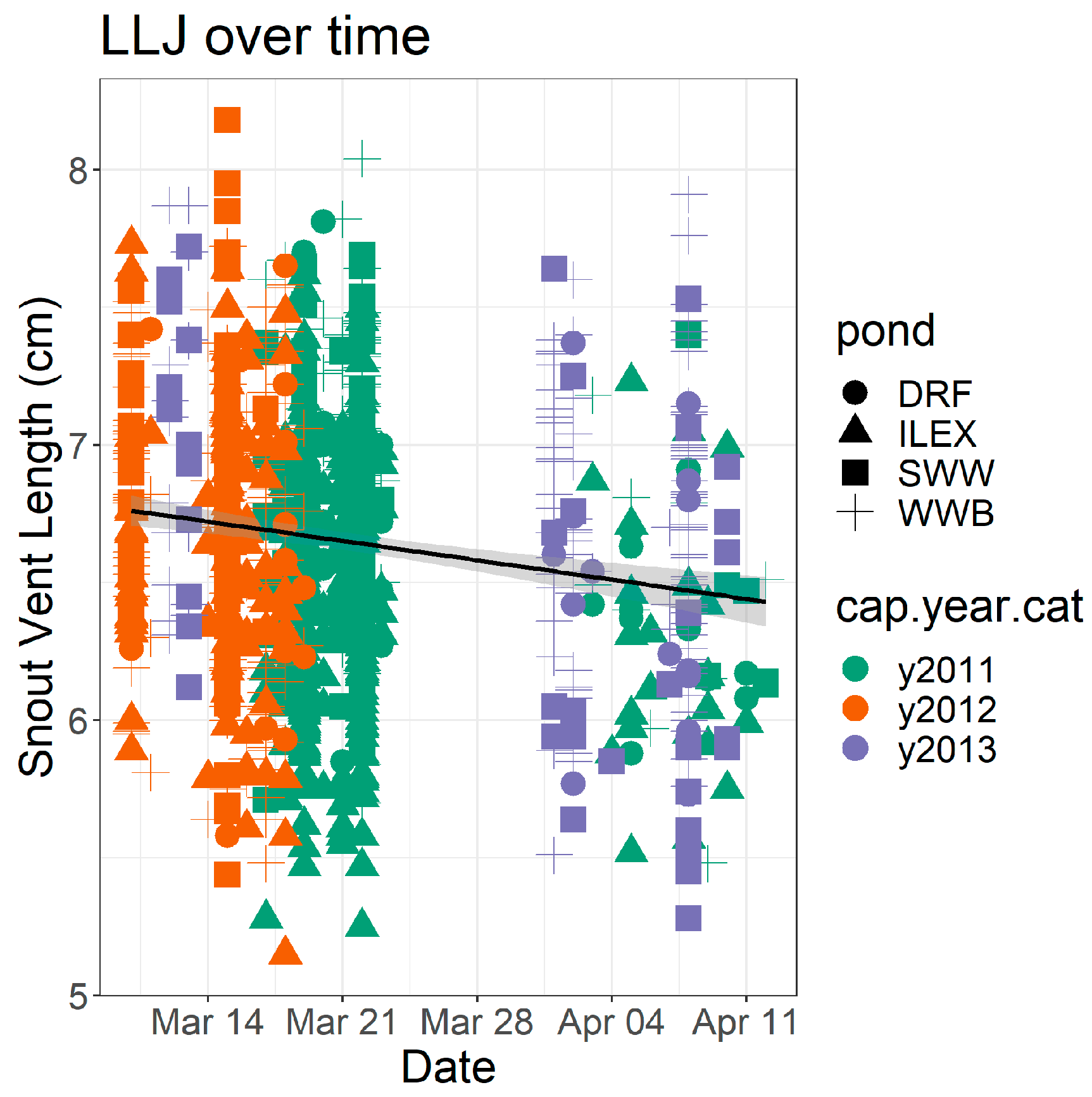
In the analysis of LLJ unisexuals captured in all three years (2011–2013), neither recapture status (Χ21 = 0.95, p = 0.32) nor body condition (Χ21 = 0.01, p = 0.93) was a predictor of ordinal date of capture. However, SVL was related to capture date, such that LLJ unisexuals with longer SVL migrated to the breeding season earlier than LLJ unisexuals with shorter SVL (Χ21 = 16.5, p < 0.0001, Figure 3).
In the analysis of factors affecting recapture status of LLJ unisexuals in 2011, body condition did not affect recapture status (Χ21 = 0.05, p = 0.81), but SVL did affect recapture status, with longer animals more likely to be eventually recaptured (Χ21 = 4.56, p = 0.03; Supplementary Materials Figure S5).
The probability of breeding migrations was affected by precipitation, temperature, and ordinal day for all amphibians, but each species and sex were affected by these factors in different ways (Table 1 and Supplementary Materials Table S2 and Figures S6–S12). For example, early in the year, A. laterale complex salamanders were more likely to migrate than female wood frogs, regardless of the temperature (Figure 4). Ambystoma laterale complex salamander immigration was associated with average maximum temperature over two days. Male tiger salamander immigration was also associated with average maximum temperature over two days, but female tiger salamander movement was associated with average maximum temperature over four or five days. Both male and female Rana sylvatica immigration were associated with the maximum temperature on the day they were captured. All of the top models included some measure of precipitation. For the Ambystoma salamanders, migration was most closely associated with precipitation on the day of capture, but for wood frogs, migration was associated with total precipitation over two or three days preceding the migration. The ordinal day of the year affected migration for all species and sexes, but the strength varied between species and sexes. The percentage of the moon illuminated was not significant in these models. Even though moon phase did appear in some of the top models, the confidence intervals for the model-averaged parameter estimates always overlapped zero (Supplementary Materials Table S2).
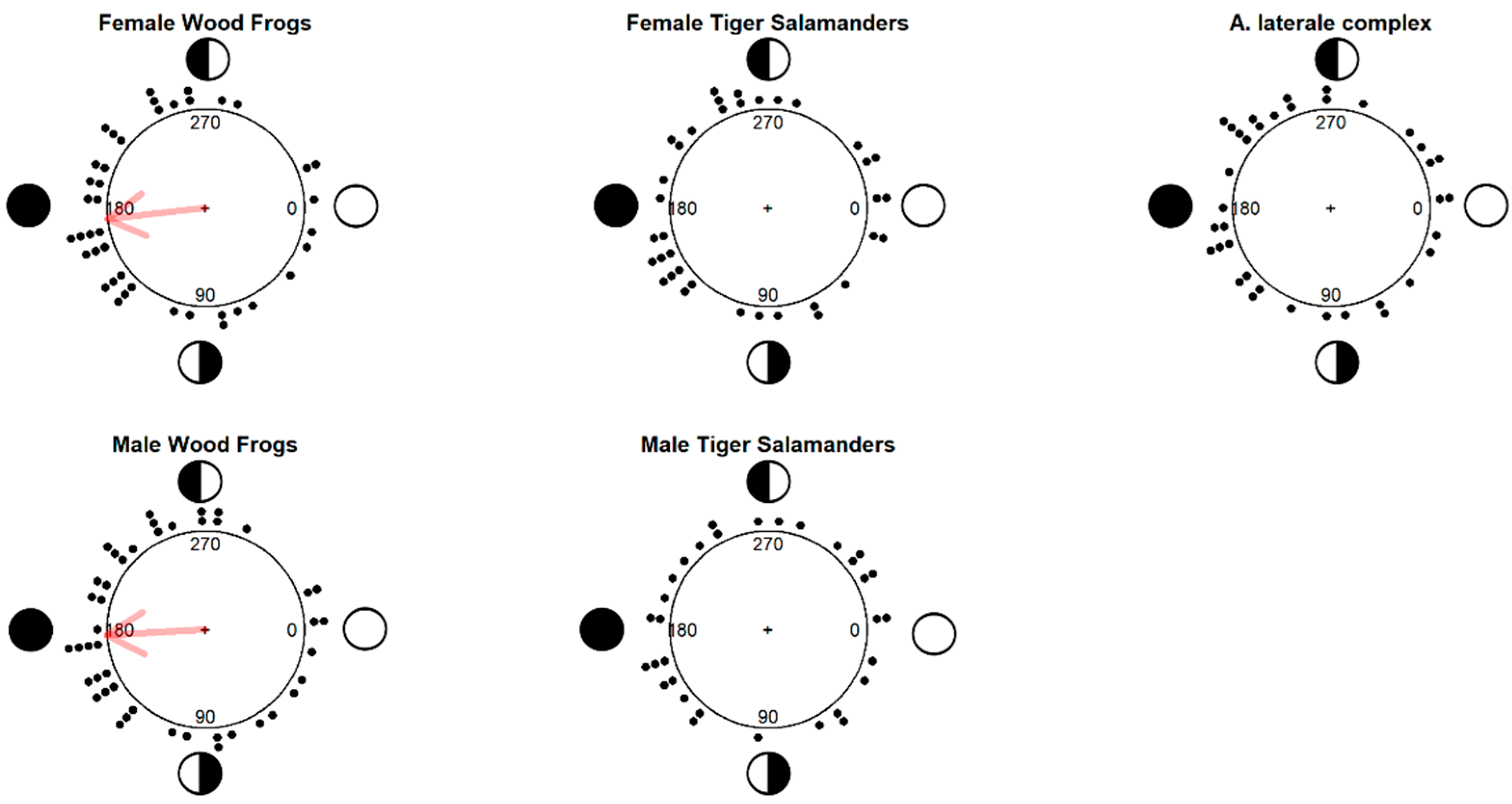
The separate analysis of amphibian migration and lunar phase using circular statistics found no association between migration and lunar phase for A. laterale complex salamanders (U = 136.2, N = 37, p > 0.10), female A. tigrinum (U = 140, N = 36, p > 0.10), nor male A. tigrinum (U = 112.5, N = 32, p > 0.10). However, female R. sylvatica (U = 162.8, N = 45, p = 0.01 to 0.05) and male R. sylvatica (U = 160, N = 45, p = 0.01 to 0.05) were more likely to migrate around the time of the new moon (Figure 5).
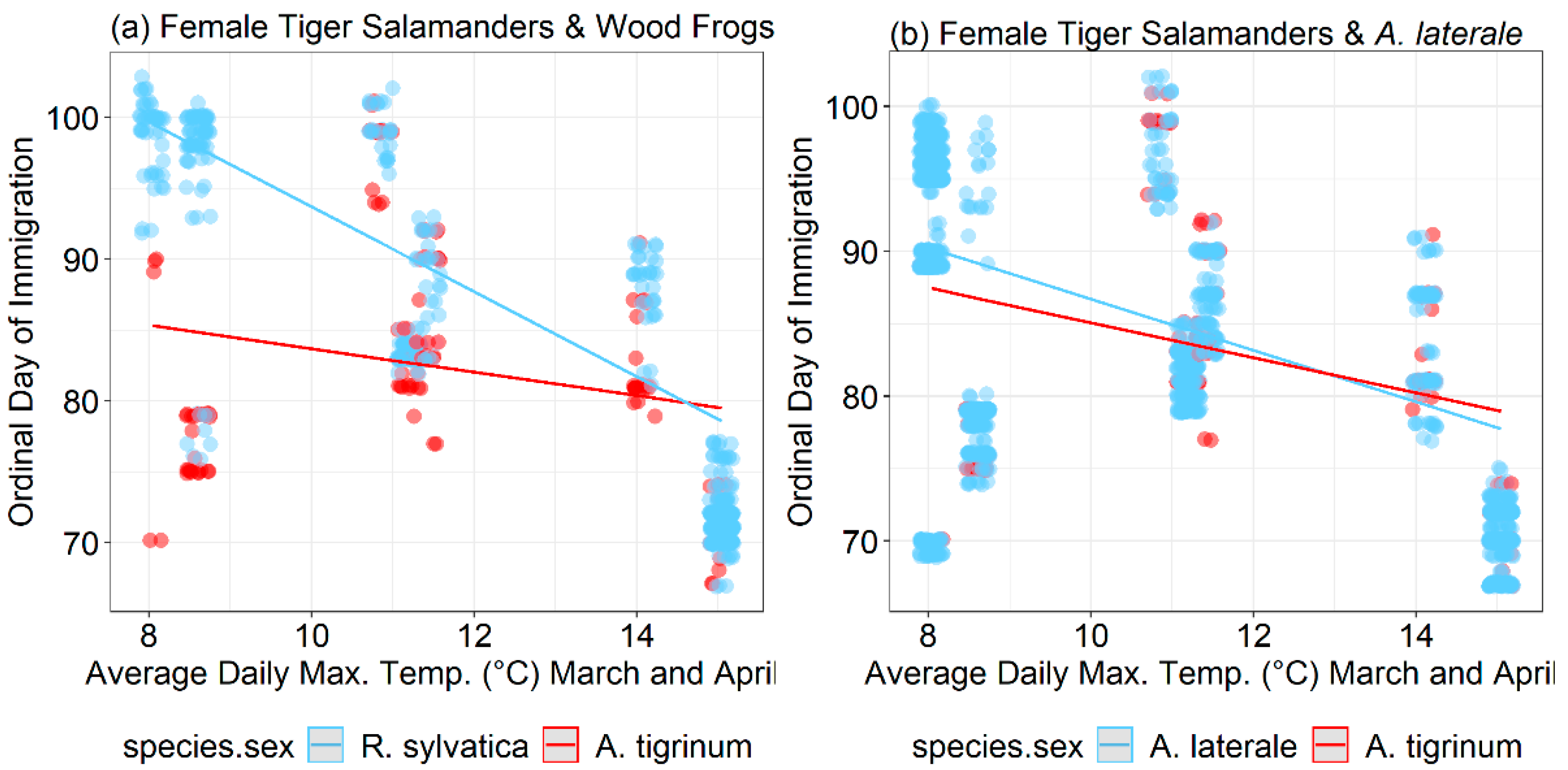
In the analysis of the timing of female wood frog and tiger salamander immigration, there was a significant interaction between species and average maximum temperature (Χ21 = 144.4, p < 0.0001). In cold years, female wood frogs arrived at wetlands on average 15 days after female tiger salamanders, but in warmer years female wood frogs and female tiger salamanders arrived simultaneously (Figure 6a). There was also an interaction between species and average maximum temperature for female tiger salamanders and A. laterale21 = 5.96, p < 0.015). This effect was similar to the previous effect with wood frogs, but it was less pronounced (Figure 6b).

4. Discussion

Our analysis provides several insights into the phenological variability of breeding in a community of amphibians. First, although there were differences among species, sexes, and biotypes in immigration date, the magnitude of differences between groups varied greatly between years. In some years the average migration date of groups differed by as many as 20 days, whereas in other years groups migrated essentially synchronously. Similarly, fine-scale geographic variation existed in the average migration date into some wetlands, but this was also dependent on year; in some years ponds differed in migration date, whereas in other years there was no difference in migration date among wetlands. Second, although temperature, precipitation, and ordinal day all affected the probability of migration in amphibians, each species-sex group had a unique set of environmental factors most likely to trigger migration. Third, as average winter temperature increased, the breeding migration of tiger salamanders, A. laterale complex salamanders, and wood frogs became increasingly synchronized. These findings have important implications for the ecology, evolution, and conservation of these amphibians in the face of a changing climate.
The absolute and relative timing of arrival differed among species, sexes, and years. Although the proximate environmental cues explaining species-specific differences in the timing of breeding migrations are being increasingly investigated, it is also valuable to understand the evolutionary explanation for these differences. There is likely strong selection on phenology from both abiotic and biotic factors. For example, absolute timing of breeding can allow species to metamorphose earlier in the year, but earlier breeding carries the cost of colder temperatures during larval development and greater risk of exposure to dangerous freeze conditions [15,66]. Similarly, changes in the relative timing of when different species breed has the potential to change the strength and nature of interspecific interactions in amphibians, which can affect fitness [67,68]. Comparing across species, earlier breeding species typically have greater cold tolerance than later breeding species, suggesting a co-evolution of these traits [69]. As the climate changes, amphibian phenology itself may also evolve in response to these shifting selection pressures, as has been documented in other organisms [70]. However, despite the strong phenological responses of amphibians to climate change, there remains little information on whether these responses are genetically based or entirely caused by phenotypic plasticity [71].
Many animals exhibit protrandry, where males arrive at breeding sites before females [72]. In our study, male wood frogs consistently arrived earlier than female wood frogs, and male A. laterale arrived earlier than both female A. laterale and unisexual salamanders. There was a non-significant trend for male tiger salamanders to arrive earlier than females. Protrandry appears to be geographically variable in tiger salamanders, where it has been documented in some populations but not others [73,74]. Earlier arrival of males has been documented in other wood frog populations [75] but is not quantified in many studies of wood frog phenology [76,77]. Multiple hypotheses have been proposed for the evolution of protrandry [72]. For example, there may be selection on males to arrive earlier to maximize the chance to mate with multiple females, or there may be selection on females to arrive later to increase the number of males that they can assess as part of mate choice [72]. Although protrandry is well studied in some taxa, it is much less well understood in amphibians [72]. Our understanding of the ecological significance and evolutionary consequences of protrandry in amphibians would benefit from both experimental studies as well as an increased reporting of the timing of breeding migration of males and females.
Geographic variation in phenological responses on relatively small spatial scales can be caused by factors including spatial variation in microclimate as well as phenotypically or genetically based differences in how individuals respond to the same environmental cues [9,78]. Despite the ecological differences in canopy cover [55,79] and its effect on amphibian growth and development [34,36,80], there was no effect of canopy cover on average breeding date. There were some years in which ponds did differ in phenology, such as 2011, when there was an approximately 10-day difference in average breeding date between the most extreme wetlands. However, in most years there was no difference in average breeding date among the six wetlands. We suspect that phenological differences in our study are due to small-scale microclimate differences; however, given local adaptation in other traits [37,81,82], genetic explanations cannot be ruled out. Recent work in plant phenology has demonstrated that in warmer years spatial microclimate differences are homogenized, increasing spatial synchrony in budbreak [9]. Although amphibians have been a bellwether for phenology shifts, no work has examined whether climate change is increasing fine-scale spatial synchrony in their breeding phenology. In other species, geographic variation in phenology can increase reproductive isolation or cause biased gene flow [28,29]. In amphibians, fine-scale differences in phenology could also have important implications for amphibian metapopulations. For instance, if phenological differences in breeding date affect larval survival or age and size at metamorphosis, that in turn could affect spatial variation in local recruitment and whether a population acts as a source or sink on the landscape.
Phenological shifts could also affect the interactions among unisexual Ambystoma biotypes and their sexual host species. As reported elsewhere (e.g., [46]), triploid unisexual females tended to arrive in advance of tetraploid females, although this pattern was not statistically significant in our study, likely due to the relatively small sample size of tetraploids. When restricting analysis to a single biotype, we found that longer (greater SVL) LLJ unisexuals moved to the ponds earlier than smaller animals. Few studies have investigated size-ordered immigration in ambystomatid salamanders, and those that have report variable results across species and regions. Smaller males arrived at breeding ponds earlier than larger males in both A. talpoideum [83] and A. tigrinum [84]; however, in the fall-breeding A. annulatum, larger animals of both sexes arrived earlier than smaller animals [85]. In contrast to Semlitsch et al. [84]’s results in South Carolina, Williams et al. [74] found no relationship between SVL and immigration in either A. tigrinum or A. texanum at a site in Indiana. Our results may be best explained by the unisexual salamander’s unique reproductive mode. Mate choice experiments show that male A. laterale prefer females of their own species, followed by LLJ and finally LJJ unisexuals [86]. If males discriminate against larger unisexual females (because they are more dissimilar to full A. laterale females), it may be adaptive for these larger females to arrive earlier to avoid direct competition for access to mates.
Across biotypes, unisexuals had much greater recapture rates (11.9% for LLJ, 10.9% for LLLJ) than pure A. laterale females (3.9%). These differences in recapture rates generate several non- exclusive hypotheses: (a) unisexual females have higher annual survivorship than A. laterale females; (b) unisexual females breed more frequently than A. laterale females; or (c) unisexual females have higher retention of PIT tags than A. laterale females. Although PIT tag retention has been shown to be problematic in previous studies of A. laterale [87], our marked A. laterale females were slightly larger on average (57.5 mm vs. 54.5 mm SVL), and our PIT tags were substantially smaller (8 mm vs. 12 mm tags) than those in the Ryan et al. (2014) study [87], which should reduce tag loss. Even with potential tag loss biased toward smaller animals, we suspect that the difference in recapture rate between A. laterale and unisexual females reflects a true difference in survival or breeding frequency. Similarly, LLJ females with larger SVL were significantly more likely to be recaptured than smaller LLJ females, and so the same hypotheses could be investigated among size classes within a biotype. The finding that larger unisexual salamanders breed earlier and are also more likely to be recaptured in subsequent years may point to important differences in life history strategy that could influence the coexistence of these sexual and unisexual lineages.
Our results provide insights into the environmental factors that trigger amphibian migrations. Similar to other studies on amphibians, temperature and precipitation were associated with migration [22,23,24]. Each species had a specific combination of temperature and precipitation lags that likely contribute to differences in the timing of migration. It is worth noting that the regional weather data we used are probably not the specific cues the amphibians are actually responding to. For example, amphibians hibernating underground are likely responding to soil temperature rather than air temperature, although the two variables are correlated [24,88]. Using regional weather data can still be valuable to predict amphibian migration but could be strengthened by a more mechanistic understanding of the links between regional weather, the specific cues amphibians detect, and how these linkages are affected by environmental factors (e.g., soil type). In some cases, these links may be complex, such as desert frogs that respond to the sound of rainfall rather than direct experience of moisture [89]. All species exhibited a significant effect on the ordinal day, with the probability of migrating increasing later in the season. We suggest two general explanations for the effect of the ordinal day. One possibility is that the ordinal day is correlated with some unmeasured environmental variable that triggers migration. An alternative possibility is that amphibians have a refractory period that prevents them from breeding too early in the season, even when conditions otherwise appear suitable for migration. Work in other species has also noted that early in winter species did not migrate despite suitable (warm and rainy) conditions [24]. Such refractory periods are likely an adaptive response to prevent migration during temporary early thaws when the threat of subsequent dangerous weather is high.
Our linear models did not find a signal of lunar phase in amphibian migrations, but the circular statistics indicated both female and male wood frogs were more likely to move to the breeding sites around the time of the new moon. Responses to lunar cues are unevenly spread across amphibians, with correlations between lunar phase and some behaviors. It is probable that different species respond to different aspects of lunar phase (e.g., illumination vs. gravitational pull), and potential adaptive explanations for this behavior include predator avoidance and synchronization of breeding behavior [27,90]. Wood frogs were more likely to migrate around the time of the new moon, which is also when illuminance is lowest. We did not have independent field measures of illuminance to include in our study, so we cannot separate if it is darkness that makes wood frogs more likely to migrate during the new moon, or if it is increased gravitational pull or variation in geomagnetic fields [27,90]. However, in other amphibians, measurements of illumination have demonstrated that illumination from the moon plays a direct role in breeding behavior [91].
Many studies now document links between metrics of breeding (migration, calling, egg observation) with metrics of annual weather (e.g., average temperature) over multiple decades [7,21,92]. These studies have played a critical role in demonstrating the rapid response of breeding phenology to climate change in many species. Relatively fewer studies quantify links between breeding and immediate environmental triggers, and many of those are of relatively short duration. Although a few studies are longer (24 years [22], 20 years [93], 10 years [24]), most others are shorter (6 years [26], 5 years [25], 4 years [23], 2 years [94], and 1 year [95]) than our seven-year study. Increasing the number of long-term studies of proximate phenological cues would have multiple benefits, including allowing comparison of geographic variation in cues and the development of predictive models of phenology.
Quantification of specific cues related to amphibian breeding migration holds promise for understanding effects of climate change but also raises questions. Mechanistic models of phenology have been widely developed for other organisms but rarely for amphibians [12,13,14]. Such models could be used to improve our understanding of past and future amphibian responses to climate change. For example, models of phenology in toads were used to infer a historical shift in breeding phenology [22]. However, application of such models must be cautious of both geographic variation and the potential for adaptation. For widely distributed species, phenological models from one population may not be applicable to distant populations due to historical adaptation to local climate. This is particularly important to consider in that phenological shifts are occurring more rapidly in northern populations compared to southern populations [10]. Even within a single population, there is a potential for species to rapidly adapt phenological responses to changing environmental conditions [70]. For example, if there is a refractory period that prevents amphibians from migrating too early in the year, then the speed at which amphibian phenology can adapt may be limited by genetic variation in the refractory period. Although the great variability in when amphibians migrate indicates that important aspects of the timing of amphibian breeding are plastic, there is little information on the relative importance of genetics vs. plasticity in amphibian phenology [71].
Climate change has the potential to alter the nature and outcome of species interactions by changing the relative phenology of different species [2,3]. Our results suggest that this is likely to occur in our system. In colder years, tiger salamanders bred earlier than wood frogs or A. laterale complex salamanders, but in warmer years the breeding of all three species is more synchronous. Relatively earlier breeding by tiger salamanders may give them a hatching growth advantage that increases their ability to prey upon wood frog and A. laterale complex larvae [39,96]. Experimental work in other systems has shown that predation rate increases as the delay between predator arrival and amphibian hatching increases, although that can be complicated by indirect effects in more complex food webs [97]. If our results from seven years of data can be extrapolated to the longer term, it suggests that in a warming climate, synchronization of the timing of breeding of these amphibians may reduce the predatory impact of tiger salamanders on their prey. The effects of synchronized breeding on tiger salamanders are less clear, as they have other food sources, including invertebrates and later-breeding amphibian species. Our findings help connect studies showing interspecific differences in the rates of phenological response to climate change [7,11,19] with experimental investigations of the effects of phenology on interspecific interactions in amphibians [6,17,18]. Combining information on known or predicted phenological shifts for interacting species with experimental manipulations allows tests of hypotheses for how climate change is likely to alter species interactions in the future [41].

Supplementary Materials

The following supporting information can be downloaded at: https://www.mdpi.com/article/10.3390/d15020253/s1. Supplementary Materials Table S1. Interpond distance (meters) between wetlands. Supplementary Materials Table S2. Model-averaged parameter estimates of relationships between weather and immigration. Species-sex abbreviations are the same as for Table 1. Estimates are only presented for variables that were present in the top models (models with delta AIC less than 2) for that species-sex combination. The estimate is presented on top, and the 95% confidence interval is presented below. Supplementary Materials Figure S1. Differences in ordinal date of arrival among six wetlands across years. There is no systematic difference between the closed-canopy wetlands (Dreadful Hollow, Southwest Woods, and West Woods Big) and the open-canopy wetlands (Ilex, Star, West Marsh 06). Supplementary Materials Figure S2. Ambystoma laterale complex capture in 2011 by wetland. Supplementary Materials Figure S3. Ambystoma laterale complex capture in 2012 by wetland. Supplementary Materials Figure S4. Ambystoma laterale complex capture in 2013 by wetland. Supplementary Materials Figure S5. Probability of recapture for LLJ unisexuals captured in 2011. Supplementary Materials Figure S6. Summary of weather conditions from 2007–2013. Gray bars indicate precipitation. The colored dots indicate average maximum daily temperature over certain lag periods (no lag, 2-day lag, 5-day lag). Supplementary Materials Figure S7. Number of immigration A. laterale complex salamanders (bars) and average maximum daily temperature over the previous two days. Supplementary Materials Figure S8. Number of immigrating female tiger salamanders (bars) versus average maximum daily temperature over the previous four days. Supplementary Materials Figure S9. Number of immigrating male tiger salamanders (bars) vs. average maximum daily temperature over the previous two days. Supplementary Materials Figure S10. Number of immigrating female wood frogs (bars) versus maximum temperature on the day of migration. Supplementary Materials Figure S11. Number of immigrating male wood frogs (bars) versus maximum temperature on the day of migration. Supplementary Materials Figure S12. Probability of breeding migration for the five amphibian species/sexes, for different combinations of temperature, precipitation and ordinal day.

Author Contributions

Conceptualization, M.F.B. and K.R.G.; methodology, M.F.B. and K.R.G.; formal analysis, M.F.B. and K.R.G.; investigation M.F.B. and K.R.G.; data curation, M.F.B. and K.R.G.; writing—original draft preparation, M.F.B. and K.R.G.; writing—review and editing M.F.B. and K.R.G.; supervision, M.F.B. and K.R.G.; project administration, M.F.B. and K.R.G.; funding acquisition, M.F.B. and K.R.G. All authors have read and agreed to the published version of the manuscript.

Funding

M.F.B. was supported during part of this research by the University of Michigan and the Michigan Society of Fellows, and Case Western Reserve University. K.R.G. was supported by Eastern Michigan University’s Faculty Research Fellowship and Undergraduate Stimulus Research Program support for students.

Institutional Review Board Statement

The research was conducted under Michigan Department of Natural Resources Scientific Collecting Permits to Michael Benard and Katherine Greenwald. This research was authorized under University of Michigan UCUCA, Case Western Reserve University IACUC, and Eastern Michigan University IACUC.

Data Availability Statement

Upon acceptance and publication of this manuscript, data will be available via DataDryad.

Acknowledgments

We thank the many colleagues who assisted with diverse aspects of this research, particularly, Paul Anderson, Tina Barbasch, Matthew Boes, Christina Casto, David Clipner, Natalie Colletti, Mathew Conger, Chris Davis, Marisa Hildebrandt, Danielle Hulvey, Katherine Krynak, Jay Krystyniak, T.J. Kunde, Letitia Jaques, Danielle Johnston, Jessica Middlemis Maher, Thomas Nuttall, Olivia Scheffler, Sarah Seiter, Kaitlyn Shott, Chase Stevens, Donn Stroud, John Vanek, Earl Werner, Andrew Zajac and Amanda Zellmer. The University of Michigan provided access to the E. S. George Reserve, and the staff of the ESGR provided valuable logistical support.

Conflicts of Interest

The authors declare no conflict of interest.

References

  1. Ramula, S.; Johansson, J.; Linden, A.; Jonzen, N. Linking phenological shifts to demographic change. Clim. Res. 2015, 63, 135–144. [Google Scholar] [CrossRef]
  2. Visser, M.E.; Gienapp, P. Evolutionary and demographic consequences of phenological mismatches. Nat. Ecol. Evol. 2019, 3, 879–885. [Google Scholar] [CrossRef]
  3. Yang, L.H.; Rudolf, V.H.W. Phenology, ontogeny and the effects of climate change on the timing of species interactions. Ecol. Lett. 2010, 13, 1–10. [Google Scholar] [CrossRef]
  4. Inouye, D.W. Effects of climate change on phenology, frost damage, and floral abundance of montane wildflowers. Ecology 2008, 89, 353–362. [Google Scholar] [CrossRef]
  5. Ozgul, A.; Childs, D.Z.; Oli, M.K.; Armitage, K.B.; Blumstein, D.T.; Olson, L.E.; Tuljapurkar, S.; Coulson, T. Coupled dynamics of body mass and population growth in response to environmental change. Nature 2010, 466, 482–485. [Google Scholar] [CrossRef]
  6. Rasmussen, N.L.; Rudolf, V.H.W. Individual and combined effects of two types of phenological shifts on predator-prey interactions. Ecology 2016, 97, 3414–3421. [Google Scholar] [CrossRef]
  7. Todd, B.D.; Scott, D.E.; Pechmann, J.H.K.; Gibbons, J.W. Climate change correlates with rapid delays and advancements in reproductive timing in an amphibian community. Proc. Royal Soc. B 2011, 278, 2191–2197. [Google Scholar] [CrossRef]
  8. Harnos, A.; Nora, A.; Kovacs, S.; Lang, Z.; Csorgo, T. Increasing protandry in the spring migration of the Pied Flycatcher (Ficedula hypoleuca) in Central Europe. J. Ornithol. 2015, 156, 543–546. [Google Scholar] [CrossRef]
  9. Ward, S.E.; Schulze, M.; Roy, B. A long-term perspective on microclimate and spring plant phenology in the Western Cascades. Ecosphere 2018, 9, e02451. [Google Scholar] [CrossRef]
  10. Cohen, J.M.; Lajeunesse, M.J.; Rohr, J.R. A global synthesis of animal phenological responses to climate change. Nat. Clim. Chang. 2018, 8, 224–228. [Google Scholar] [CrossRef]
  11. Parmesan, C. Influences of species, latitudes and methodologies on estimates of phenological response to global warming. Glob. Chang. Biol. 2007, 13, 1860–1872. [Google Scholar] [CrossRef]
  12. Chuine, I.; Regniere, J. Process-Based Models of Phenology for Plants and Animals. Annu. Rev. Ecol. Evol. Syst. 2017, 48, 159–182. [Google Scholar] [CrossRef]
  13. Helm, B.; Ben-Shlomo, R.; Sheriff, M.J.; Hut, R.A.; Foster, R.; Barnes, B.M.; Dominoni, D. Annual rhythms that underlie phenology: Biological time-keeping meets environmental change. Proc. Royal Soc. B 2013, 280, 20130016. [Google Scholar] [CrossRef]
  14. Simmonds, E.G.; Cole, E.F.; Sheldon, B.C. Cue identification in phenology: A case study of the predictive performance of current statistical tools. J. Anim. Ecol. 2019, 88, 1428–1440. [Google Scholar] [CrossRef]
  15. Benard, M.F. Warmer winters reduce frog fecundity and shift breeding phenology, which consequently alters larval development and metamorphic timing. Glob. Chang. Biol. 2015, 21, 1058–1065. [Google Scholar] [CrossRef]
  16. Loman, J. Primary and secondary phenology. Does it pay a frog to spawn early? J. Zool. 2009, 279, 64–70. [Google Scholar] [CrossRef]
  17. Anderson, T.L.; Rowland, F.E.; Semlitsch, R.D. Variation in phenology and density differentially affects predator-prey interactions between salamanders. Oecologia 2017, 185, 475–486. [Google Scholar] [CrossRef]
  18. Lawler, S.P.; Morin, P.J. Temporal overlap, competition, and priority effects in larval anurans. Ecology 1993, 74, 174–182. [Google Scholar] [CrossRef]
  19. Gibbs, J.P.; Breisch, A.R. Climate warming and calling phenology of frogs near Ithaca, New York, 1900–1999. Conserv. Biol. 2001, 15, 1175–1178. [Google Scholar] [CrossRef]
  20. Klaus, S.P.; Lougheed, S.C. Changes in breeding phenology of eastern Ontario frogs over four decades. Ecol. Evol. 2013, 3, 835–845. [Google Scholar] [CrossRef]
  21. While, G.M.; Uller, T. Quo vadis amphibia? Global warming and breeding phenology in frogs, toads and salamanders. Ecography 2014, 37, 921–929. [Google Scholar] [CrossRef]
  22. Green, D.M. Amphibian breeding phenology trends under climate change: Predicting the past to forecast the future. Glob. Chang. Biol. 2017, 23, 646–656. [Google Scholar] [CrossRef] [PubMed]
  23. Semlitsch, R.D. Analysis of Climatic Factors Influencing Migrations of the Salamander Ambystoma talpoideum. Copeia 1985, 1985, 477. [Google Scholar] [CrossRef]
  24. Sexton, O.J.; Phillips, C.; Bramble, J.E. The effects of temperature and precipitation on the breeding migration of the spotted salamander (Ambystoma maculum). Copeia 1990, 1990, 781–787. [Google Scholar] [CrossRef]
  25. Timm, B.C.; McGarigal, K.; Compton, B.W. Timing of large movement events of pond-breeding amphibians in Western Massachusetts, USA. Biol. Conserv. 2007, 136, 442–454. [Google Scholar] [CrossRef]
  26. Brooks, G.C.; Smith, J.A.; Gorman, T.A.; Haas, C.A. Discerning the Environmental Drivers of Annual Migrations in an Endangered Amphibian. Copeia 2019, 107, 270–276. [Google Scholar] [CrossRef]
  27. Grant, R.A.; Chadwick, E.A.; Halliday, T. The lunar cycle: A cue for amphibian reproductive phenology? Anim. Behav. 2009, 78, 349–357. [Google Scholar] [CrossRef]
  28. Adamski, P.; Ćmiel, A.M.; Lipińska, A.M. Intraseasonal asynchrony as a factor boosting isolation within a metapopulation: The case of the clouded apollo. Insect. Sci. 2019, 26, 911–922. [Google Scholar] [CrossRef]
  29. Stanton, M.L.; Galen, C. Life on the edge: Adaptation versus environmentally mediated gene flow in the snow buttercup, Ranunculus adoneus. Am. Nat. 1997, 150, 143–178. [Google Scholar] [CrossRef]
  30. Marsh, D.M.; Fegraus, E.H.; Harrison, S. Effects of breeding pond isolation on the spatial and temporal dynamics of pond use by the tungara frog, Physalaemus pustulosus. J. Anim. Ecol. 1999, 68, 804–814. [Google Scholar] [CrossRef]
  31. Smith, M.A.; Green, D.M. Dispersal and the metapopulation paradigm in amphibian ecology and conservation: Are all amphibian populations metapopulations? Ecography 2005, 28, 110–128. [Google Scholar] [CrossRef]
  32. Werner, E.E.; Yurewicz, K.L.; Skelly, D.K.; Relyea, R.A. Turnover in an amphibian metacommunity: The role of local and regional factors. Oikos 2007, 116, 1713–1725. [Google Scholar] [CrossRef]
  33. Takahashi, K.; Sato, T. Spatial variation in breeding phenology at small spatial scales: A stochastic effect of population size. Popul. Ecol. 2020, 62, 332–340. [Google Scholar] [CrossRef]
  34. Boes, M.W.; Benard, M.F. Carry-Over Effects in Nature: Effects of Canopy Cover and Individual Pond on Size, Shape and Locomotor Performance of metamorphosing Wood Frogs. Copeia 2013, 2013, 717–722. [Google Scholar] [CrossRef]
  35. Freidenburg, L.K.; Skelly, D.K. Microgeographical variation in thermal preference by an amphibian. Ecol. Lett. 2004, 7, 369–373. [Google Scholar] [CrossRef]
  36. Halverson, M.A.; Skelly, D.K.; Kiesecker, J.M.; Freidenburg, L.K. Forest mediated light regime linked to amphibian distribution and performance. Oecologia 2003, 134, 360–364. [Google Scholar] [CrossRef]
  37. Relyea, R.A. Local population differences in phenotypic plasticity: Predator-induced changes in wood frog tadpoles. Ecol. Monogr. 2002, 72, 77–93. [Google Scholar] [CrossRef]
  38. Wilbur, H.M. Competition, predation and structure of Ambystoma-Rana sylvatica community. Ecology 1972, 53, 3–21. [Google Scholar] [CrossRef]
  39. Sredl, M.J.; Collins, J.P. The effect of ontogeny on interspecific interactions in larval amphibians. Ecology 1991, 72, 2232–2239. [Google Scholar] [CrossRef]
  40. Berven, K.A. Factors affecting variation in reproductive traits within a population of wood frogs (Rana sylvatica). Copeia 1988, 1998, 605–615. [Google Scholar] [CrossRef]
  41. Rollins, H.B.; Benard, M.F. Challenges in predicting the outcome of competition based on climate change-induced phenological and body size shifts. Oecologia 2020, 193, 749–759. [Google Scholar] [CrossRef] [PubMed]
  42. Bogart, J.P.; Bi, K.; Fu, J.Z.; Noble, D.W.A.; Niedzwiecki, J. Unisexual salamanders (genus Ambystoma) present a new reproductive mode for eukaryotes. Genome 2007, 50, 119–136. [Google Scholar] [CrossRef] [PubMed]
  43. Bogart, J.P.; Bartoszek, J.; Noble, D.W.A.; Bi, K. Sex in unisexual salamanders: Discovery of a new sperm donor with ancient affinities. Heredity 2009, 103, 483–493. [Google Scholar] [CrossRef] [PubMed]
  44. Brodman, R.; Krouse, H.D. How blue-spotted and small-mouthed salamander larvae coexist with their unisexual counterparts. Herpetologica 2007, 63, 135–143. [Google Scholar] [CrossRef]
  45. Greenwald, K.R.; Denton, R.D.; Gibbs, H.L. Niche partitioning among sexual and unisexual Ambystoma salamanders. Ecosphere 2016, 7, e01579. [Google Scholar] [CrossRef]
  46. Lowcock, L.A. Biotype, genomotype, and genotype: Variable effects of polyploidy and hybridity on ecological partitioning in a bisexual-unisexual community of salamanders. Can. J. Zool. 1994, 72, 104–117. [Google Scholar] [CrossRef]
  47. Van Drunen, S.G.; Linton, J.E.; Bogart, J.P.; McCarter, J.; Fotherby, H.; Sandilands, A.; Norris, D.R. Estimating critical habitat based on year-round movements of the endangered jefferson salamander (Ambystoma jeffersonianum) and their unisexual dependents. Can. J. Zool. 2020, 98, 117–126. [Google Scholar] [CrossRef]
  48. Bogart, J.P.; Klemens, M.W. Additional distributional records of Ambystoma laterale, A-jeffersonianum (Amphibia: Caudata) and their unisexual kleptogens in northeastern North America. Am. Mus. Novit. 2008, 2008, 1–58. [Google Scholar] [CrossRef]
  49. Bogart, J.P.; Klemens, M.W. Hybrids and genetic interactions of mole salamanders (Ambystoma jeffersonianum and A. laterale) (Amphibia, Caudata) in New York and New England. Am. Mus. Novit. 1997, 3218. [Google Scholar]
  50. Phillips, C.A.; Uzzell, T.; Spolsky, C.M.; Serb, J.M.; Szafoni, R.E.; Pollowy, T.R. Persistent high levels of tetraploidy in salamanders of the Ambystoma jeffersonianum complex. J. Herpetol. 1997, 31, 530. [Google Scholar] [CrossRef]
  51. Licht, L.E.; Bogart, J.P. Growth and sexual maturation in diploid and polyploid salamanders (Genus Ambstyoma). Can. J. Zool. 1989, 67, 812–818. [Google Scholar] [CrossRef]
  52. Lowcock, L.A.; Griffith, H.; Murphy, R.W. The Ambystoma laterale-jeffersonianum complex in central ontario: Ploidy structure, sex ratio, and breeding dynamics in a bisexual-unisexual community. Copeia 1991, 1991, 87. [Google Scholar] [CrossRef]
  53. Dawley, E.M.; Dawley, R.M. Species discrimination by chemical cues in a unisexual-bisexual complex of salamanders. J. Herpetol. 1986, 20, 114. [Google Scholar] [CrossRef]
  54. Uzzell, T.M., Jr. Relations of the diploid and triploid species of the Ambystoma jeffersonianum Complex (Amphibia, Caudata). Copeia 1964, 1964, 257–300. [Google Scholar] [CrossRef]
  55. Werner, E.E.; Skelly, D.K.; Relyea, R.A.; Yurewicz, K.L. Amphibian species richness across environmental gradients. Oikos 2007, 116, 1697–1712. [Google Scholar] [CrossRef]
  56. Ramsden, C.; Beriault, K.; Bogart, J.P. A nonlethal method of identification of Ambystoma laterale, Ambystoma jeffersonianum and sympatric unisexuals. Mol. Ecol. Notes. 2006, 6, 261–264. [Google Scholar] [CrossRef]
  57. Teltser, C.; Greenwald, K.R. Survivorship of ploidy-variable unisexual ambystoma salamanders across developmental stages. Herpetologica 2015, 71, 81–87. [Google Scholar] [CrossRef]
  58. Julian, S.E.; King, T.L. Novel tetranucleotide microsatellite DNA markers for the wood frog, Rana sylvatica. Mol Ecol. Notes. 2003, 3, 256–258. [Google Scholar] [CrossRef]
  59. Lowcock, L.A.; Licht, L.E.; Bogart, J.P. Nomenclature in hybrid complexes of Ambystoma (Urodela, Ambystomatidae)-No case for the erection of hybrid species. Syst. Zool. 1987, 36, 328–336. [Google Scholar] [CrossRef]
  60. Lenth, R.V. Emmeans: Estimated Marginal Means, Aka Least-Squares Means. R Package 1.7.2. In R Foundation for Statistical Computing; 2022; Volume 34. [Google Scholar]
  61. R Core Team. R: A Language and Environment for Statistical Computing. 2021. R Foundation for Statistical Computing, Vienna, Austria. Available online: https://www.R-project.org/ (accessed on 4 October 2022).
  62. Bates, D.; Mächler, M.; Bolker, B.; Walker, S. Fitting linear mixed-effects models using lme4. J. Stat. Softw. 2015, 67, 1–48. [Google Scholar] [CrossRef]
  63. Hartig, F. DHARMa: Residual Diagnostics for Hierarchical (Multi-Level/Mixed) Regression Models. 2022. Available online: https://cran.r-project.org/package=DHARMa (accessed on 4 October 2022).
  64. Mazerolle, M.J. AICcmodavg: Model Selection and Multimodel Inference Based on (Q)AIC(c). 2020. Available online: https://cran.r-project.org/package=AICcmodavg (accessed on 4 October 2022).
  65. Agostinelli, C.; Lund, U. R Package “Circular”: Circular Statistics (Version 0.4-93). 2017. Available online: https://r-forge.r-project.org/projects/circular/ (accessed on 4 October 2022).
  66. Buss, N.; Swierk, L.; Hua, J. Amphibian breeding phenology influences offspring size and response to a common wetland contaminant. Front. Zool. 2021, 18, 31. [Google Scholar] [CrossRef] [PubMed]
  67. Carter, S.K.; Saenz, D.; Rudolf, V.H.W. Shifts in phenological distributions reshape interaction potential in natural communities. Ecol. Lett. 2018, 21, 1143–1151. [Google Scholar] [CrossRef] [PubMed]
  68. Carter, S.K.; Rudolf, V.H.W. Shifts in phenological mean and synchrony interact to shape competitive outcomes. Ecology 2019, 100, e02826. [Google Scholar] [CrossRef] [PubMed]
  69. John-Alder, H.B.; Morin, P.J.; Lawler, S. Thermal physiology, phenology and distribution of tree frogs. Am. Nat. 1988, 132, 506–520. [Google Scholar] [CrossRef]
  70. Bradshaw, W.E.; Holzapfel, C.M. Genetic shift in photoperiodic response correlated with global warming. Proc. Natl. Acad. Sci. USA 2001, 98, 14509–14511. [Google Scholar] [CrossRef] [PubMed]
  71. Urban, M.C.; Richardson, J.L.; Freidenfelds, N.A. Plasticity and genetic adaptation mediate amphibian and reptile responses to climate change. Evol. Appl. 2014, 7, 88–103. [Google Scholar] [CrossRef]
  72. Morbey, Y.E.; Ydenberg, R.C. Protandrous arrival timing to breeding areas: A review. Ecol. Lett. 2001, 4, 663–673. [Google Scholar] [CrossRef]
  73. Semlitsch, R.D. Structure and Dynamics of Two Breeding Populations of the Eastern Tiger Salamander, Ambystoma tigrinum. Copeia 1983, 1983, 608. [Google Scholar] [CrossRef]
  74. Williams, R.N.; Gopurenko, D.; Kemp, K.R.; Williams, B.; DeWoody, J.A. Breeding chronology, sexual dimorphism, and genetic diversity of congeneric ambystomatid salamanders. J. Herpetol. 2009, 43, 438–449. [Google Scholar] [CrossRef]
  75. Semlitsch, R.D.; Drake, D.L. Structure and dynamics of Lithobates sylvaticus (Wood Frog) at the periphery of its range in Missouri. Southeast. Nat. 2015, 14, 329–341. [Google Scholar] [CrossRef]
  76. Hocking, D.J.; Rittenhouse, T.A.G.; Rothermel, B.B.; Johnson, J.R.; Conner, C.A.; Harper, E.B.; Semlitsch, R.D. Breeding and recruitment phenology of amphibians in Missouri oak-hickory forests. Am. Midl. Nat. 2008, 160, 41–60. [Google Scholar] [CrossRef]
  77. Paton, P.; Stevens, S.; Longo, L. Seasonal phenology of amphibian breeding and recruitment at a pond in Rhode Island. Northeast. Nat. 2000, 7, 255. [Google Scholar] [CrossRef]
  78. Buchinger, T.J.; Hondorp, D.W.; Krueger, C.C. Local diversity in phenological responses of migratory lake sturgeon to warm winters. Oikos 2022, 2022, e08977. [Google Scholar] [CrossRef]
  79. Schiesari, L. Pond canopy cover: A resource gradient for anuran larvae. Freshw. Biol. 2006, 51, 412–423. [Google Scholar] [CrossRef]
  80. Werner, E.E.; Glennemeier, K.S. Influence of forest canopy cover on the breeding pond distributions of several amphibian species. Copeia 1999, 1999, 1–12. [Google Scholar] [CrossRef]
  81. Skelly, D.K. Microgeographic countergradient variation in the wood frog, Rana sylvatica. Evolution 2004, 58, 160–165. [Google Scholar]
  82. Urban, M.C. Microgeographic adaptations of spotted salamander morphological defenses in response to a predaceous salamander and beetle. Oikos 2010, 119, 646–658. [Google Scholar] [CrossRef]
  83. Hardy, L.M.; Raymond, L.R. The breeding migration of the mole salamander, Ambystoma talpoideum,in Louisiana. J. Herpetol. 1980, 14, 327. [Google Scholar] [CrossRef]
  84. Semlitsch, R.D.; Scott, D.E.; Pechmann, J.H.K.; Gibbons, J.W. Phenotypic variation in the arrival time of breeding salamanders-individual repeatability and environmental influences. J. Anim. Ecol. 1993, 62, 334–340. [Google Scholar] [CrossRef]
  85. Briggler, J.T.; Johnson, J.E.; Rambo, D.D. Demographics of a ringed salamander (Ambystoma annulatum) breeding migration. Southwest. Nat. 2004, 49, 209–217. [Google Scholar] [CrossRef]
  86. Uzzell, T.M.; Goldblatt, S.M. Serum Proteins of Salamanders of the Ambystoma jeffersonianum Complex, and the Origin of the Triploid Species of this Group. Evolution 1967, 21, 345. [Google Scholar] [CrossRef] [PubMed]
  87. Ryan, K.J.; Zydlewski, J.D.; Calhoun, A.J.K. Using Passive Integrated Transponder (PIT) systems for terrestrial detection of blue-spotted salamanders (Ambystoma laterale) in situ. Herpetol. Conserv. Biol. 2014, 9, 97–105. [Google Scholar]
  88. Van Gelder, J.J.; Olders, J.H.J.; Bosch, J.W.G.; Starmans, P.W. Behavior and body temperature of the hibernating common toads Bufo bufo. Holarct. Ecol. 1986, 9, 225–228. [Google Scholar]
  89. Marquez, R.; Beltran, J.F.; Llusia, D.; Penna, M.; Narins, P.M. Synthetic rainfall vibrations evoke toad emergence. Curr. Biol. 2016, 26, R1270–R1271. [Google Scholar] [CrossRef] [Green Version]
  90. Grant, R.; Halliday, T.; Chadwick, E. Amphibians’ response to the lunar synodic cycle-a review of current knowledge, recommendations, and implications for conservation. Behav. Ecol. 2013, 24, 53–62. [Google Scholar] [CrossRef]
  91. Onorati, M.; Vignoli, L. The darker the night, the brighter the stars: Consequences of nocturnal brightness on amphibian reproduction. Biol. J. Linn. 2017, 120, 961–976. [Google Scholar] [CrossRef]
  92. Beebee, T.J.C. Amphibian breeding and climate. Nature 1995, 374, 219–220. [Google Scholar] [CrossRef]
  93. Arietta, A.Z.A.; Freidenburg, L.K.; Urban, M.C.; Rodrigues, S.B.; Rubinstein, A.; Skelly, D.K. Phenological delay despite warming in wood frog Rana sylvatica reproductive timing: A 20-year study. Ecography 2020, 43, 1791–1800. [Google Scholar] [CrossRef]
  94. Vasconcelos, D.; Calhoun, A.J.K. Movement patterns of adult and juvenile Rana sylvatica (LeConte) and Ambystoma maculatum (Shaw) in three restored seasonal pools in Maine. J. Herpetol. 2004, 38, 551–561. [Google Scholar] [CrossRef]
  95. Todd, B.D.; Winne, C.T. Ontogenetic and interspecific variation in timing of movement and responses to climatic factors during migrations by pond-breeding amphibians. Can. J. Zool. 2006, 84, 715–722. [Google Scholar] [CrossRef]
  96. Boone, M.D.; Scott, D.E.; Niewiarowski, P.H. Effects of hatching time for larval ambystomatid salamanders. Copeia 2002, 2002, 511–517. [Google Scholar] [CrossRef]
  97. Alford, R.A. Variation in predator phenology affects predator performance and prey community composition. Ecology 1989, 70, 206–219. [Google Scholar] [CrossRef]
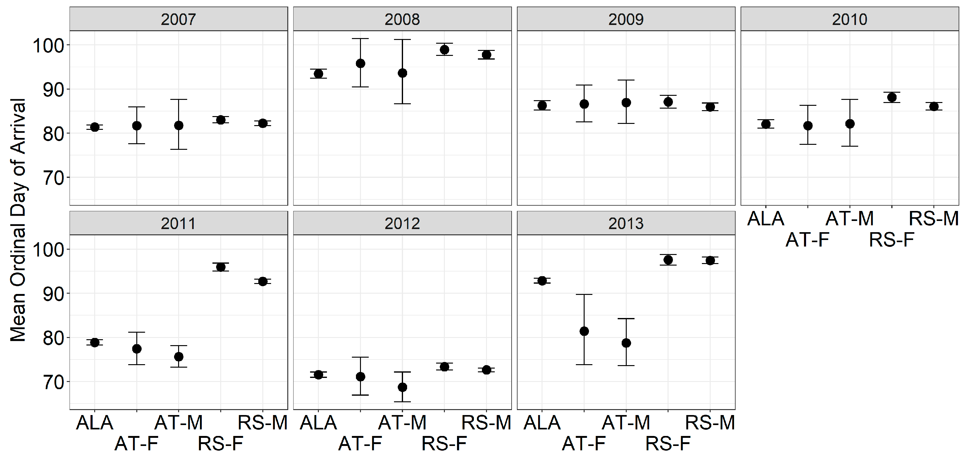
Figure 1. Variation in the ordinal date of arrival among species, sexes, and year. Points are means with 95% confidence intervals. Abbreviations are ALA = A. laterale complex, AT-F: female A. tigrinum, AT-M: male A. tigrinum, RS-F: female Rana sylvatica, RS-M: male Rana sylvatica. Ordinal Day 70 is 11 March, and Ordinal Day 100 is 10 April.
Diversity 15 00253 g001
Figure 2. Immigration date of A. laterale complex salamanders. LL_F: female A. laterale; LL_M: male A. laterale; LLJ: triploid unisexuals; LLLJ: tetraploid unisexuals.
Diversity 15 00253 g002
Figure 3. Immigration date of A. laterale complex salamanders. LLJ: triploid unisexuals.
Diversity 15 00253 g003
Figure 4. Example of how the probability of breeding migration for two amphibians (left: A. laterale complex; right: female wood frogs) responds differently to temperature, precipitation, and the ordinal day of the year.
Diversity 15 00253 g004
Figure 5. Circle plot of amphibians and moon phase. In these figures, 0° is the full moon and 180° is the new moon. Red arrows indicate statistically significant immigration associated with the new moon for female and male wood frogs.
Diversity 15 00253 g005
Figure 6. Ordinal date of immigration as a function of average March and April maximum daily temperature comparing (a) female tiger salamanders and wood frogs and (b) female tiger salamanders and A. laterale complex.
Diversity 15 00253 g006
Table 1. The best-supported models relating weather to amphibian migration. For each species-sex combination, the models with a delta AICc of less than 2 are presented. Species and sex identifications are Alat = Ambystoma laterale, Atig = A. tigrinum, Rsyl = Rana sylvatica, F = female, M = male. The number following each model represents the order of support for each model from best supported (1) to less supported. Temperature lag is the average of maximum daily temperature and ranges from maximum temperature on the day of migration to average maximum temperature over 5 days preceding migration. Similarly, precipitation is the total amount of migration ranging from precipitation only on the day of migration to the sum of precipitation over 4 days. Ordinal Day indicates that the ordinal day was a factor in the model. Moon indicates the presence of the moon in the model. For the Moon column, “no” indicates that it was not included in that model, and “NS” indicates that the model-average parameters for moon overlapped zero. K is the number of parameters in each model.
Species-Sex ModelTemp. LagPrecip. LagOrd. DayMoonKAICcDelta AICcAICc Wt
Alat 12-day meanday of mig.yesno5732.990.000.60
Alat 22-day meanday of mig.yesNS7734.791.800.24
Atig F 14-day meanday of mig.yesno5204.710.000.28
Atig F 25-day meanday of mig.yesno5205.040.330.24
Atig F 34-day meanday of mig.yesNS7206.131.420.14
Atig F 45-day meanday of mig.yesNS7206.311.600.13
Atig M 12-day meanday of mig.yesno5203.770.000.29
Atig M 22-day meanday of mig.yesNS7204.150.380.24
Rsyl F 1day of migration3-day sumyesNS8517.630.000.28
Rsyl F 2day of migration3-day sumyesno6518.240.600.21
Rsyl F 3day of migration2-day sumyesNS8518.240.600.21
Rsyl F 4day of migration2-day sumyesno6519.291.660.12
Rsyl M 1day of migration2-day sumyesno5609.750.000.28
Rsyl M 2day of migration3-day sumyesno5610.190.440.22
Rsyl M 3day of migration2-day sumyesNS7610.791.050.16
Rsyl M 4day of migration3-day sumyesNS7611.471.720.12
Rsyl M 5day of migration4-day sumyesno5611.531.780.11
Disclaimer/Publisher’s Note: The statements, opinions and data contained in all publications are solely those of the individual author(s) and contributor(s) and not of MDPI and/or the editor(s). MDPI and/or the editor(s) disclaim responsibility for any injury to people or property resulting from any ideas, methods, instructions or products referred to in the content.