Article

Time-Series Analysis of Oxygen as an Important Environmental Parameter for Monitoring Diversity Hotspot Ecosystems: An Example of a River Sinking into the Karst Underground

by
Saptashwa Bhattacharyya
1,
Janez Mulec
2,3,* and
Andreea Oarga-Mulec
4
1
Centre for Astrophysics and Cosmology, University of Nova Gorica, Vipavska 11c, SI-5270 Ajdovščina, Slovenia
2
Karst Research Institute, Research Centre of the Slovenian Academy of Sciences and Arts, Titov trg 2, SI-6230 Postojna, Slovenia
3
UNESCO Chair on Karst Education, University of Nova Gorica, Glavni trg 8, SI-5271 Vipava, Slovenia
4
Materials Research Laboratory, University of Nova Gorica, Vipavska 11c, SI-5270 Ajdovščina, Slovenia
*
Author to whom correspondence should be addressed.
Diversity 2023, 15(2), 156; https://doi.org/10.3390/d15020156
Submission received: 13 November 2022 / Revised: 17 January 2023 / Accepted: 18 January 2023 / Published: 21 January 2023

Abstract

:
Predicting variations in dissolved oxygen concentration (DO) is important for management and environmental monitoring of aquatic ecosystems. Regression analyses and univariate and multivariate time-series analyses based on autoregressive methods were performed to investigate oxygen conditions in the Pivka River, Slovenia. The monitoring site was established upstream where the river sinks into the karst cave Postojnska jama, which hosts one of the richest subterranean faunas yet studied worldwide. It was found that abnormal variations of DO started to be noticeable at values of DO < 3 mg/L and became more pronounced until the ecosystem reached fully anoxic conditions. The abnormal fluctuations during the critical summer period were due to environmental conditions, organic load and resident biota. Predictions for future detection of anomalies in DO values were made from stable residuals of the measured data, and it was demonstrated that the model could be used to obtain a reliable estimate for a short period, such as one day. The example presented an analysis pipeline based on specific and established threshold DO values, and it is particularly important for ecosystems with diversity hotspots where prolonged low DO values can pose a threat to their biota.

Graphical Abstract

1. Introduction

Oxygen is produced during photosynthesis and its presence is essential for the survival and growth of aerobic organisms, making it a critical parameter to be considered when making decisions about the water quality and ecology management of water bodies [1]. On a large scale, the expansion of oxygen-depleted zones can lead to increased N2O production, structural changes in food webs, and negative impacts on biogeochemical, physiological, and ecological processes, as well as food security and livelihoods [2]. Direct measurements around the world have shown that increases in nutrient and organic matter loading generally lead to decreases in oxygen, not only in rivers, but also in coastal areas and open oceans, resulting in a range of environmental consequences [3]. Low levels of dissolved oxygen (DO) cause stress to many organisms, and aerobic organisms die if the oxygen deficiency is prolonged. Lack of oxygen impairs ATP production; for example, almost all plants switch from mitochondrial respiration to fermentation [4]. Additionally, at low DO levels, metabolic pathways with high ATP yield are not utilized by groundwater crustaceans. These organisms are more resistant to hypoxia than are their epigean counterpart species. For example, the lethal time for 50% of the population at DO < 0.01 mg/L ranges from 46.7 to 61.7 h, and they display a better ability to recover rapidly from anoxic stress [5]. The cave-dwelling aquatic salamander Proteus anguinus, endemic to aquifers in the Dinaric karst, is one the most anoxia-tolerant amphibian species (exhibiting 50% lethal time for the population in anoxia of about 12 h, at 12 °C) and is also recognized as one of the most anoxia-tolerant vertebrates yet studied [6]. The precise values of DO in aquatic ecosystems, both on the land surface and underground, are therefore critical for estimating oxygen availability for uptake by biota.
Oxygen solubility is a function of temperature and salinity [7]; oxygen input to aquatic ecosystems is mainly through reaeration and photosynthetic production, whereas respiration is the main oxygen sink [8]. Organic pollution leads to eutrophication and microbial blooms that consume DO. Such events lead to the deterioration of living conditions for much of the indigenous biota. Here, we present a study of one such example: the ecosystem of the Pivka River, which sinks into the karst cave Postojnska jama (Slovenia). The cave harbours one of the richest aquatic and terrestrial subterranean faunas in the world, including the European cave salamander P. anguinus [9,10]. Although groundwater-dwelling faunas appear relatively resistant to low DO and to the effects of prolonged periods of hypoxia [5], establishing conditions that lead to or support prolonged periods of oxygen deficiency in aquatic ecosystems should be avoided whenever possible. Monitoring and maintaining an appropriate level of DO is particularly crucial in vulnerable habitats and those hosting endangered or endemic organisms. In 2016, the recognition that organic pollution of the Pivka River was complemented by low DO levels, prompted the introduction of a DO monitoring system at the critical point—upstream of where the river passes underground.
Variations in DO can be difficult to assess directly [11], but significant efforts are underway to develop new data-driven paradigms and predictive models for DO in relation to environmental variables [12,13,14]. There is an obvious need to improve analytical and predictive models at local scales and at large spatial and temporal scales that are important for informing ecosystem services. Next-generation models based on in situ observations and measurements, and their understanding at many scales, could simulate oxygen losses and help to identify pollution sources, impacts, and stressors that ultimately need to be managed to prevent diverse ecosystems suffering from low-oxygen conditions.
The objectives of the study were to determine the variability of DO, relate it to environmental conditions, and develop and test an analysis pipeline to support alerting the authorities if significant changes are recorded. To achieve the objectives, various data analyses techniques were applied to the collected field data, including linear regression and, for time dependent variations of DO, univariate and multivariate time-series analyses based on autoregressive methods. The main focus was on testing different time-series analysis methods and developing a real-time data monitoring model that can detect DO outliers—defined as anomalies in the dataset—automatically. The hydrological and atmospheric input data used for the analyses (from 2017 and 2020) covered the same annual period but differed distinctly in the amount of precipitation recorded.

2. Materials and Methods

2.1. Site Description

The course of the Pivka River in southwestern Slovenia extends for approximately 23 km from its source at Zagorje (N 45.6389 E 14.2281, 555 m a.s.l.) to Postojnska jama (Postojna Cave), where it sinks into the karst underground. Its upper reaches are recharged from a karst aquifer, mostly comprising Cretaceous limestone [15], within the Javorniki Mountains. In the lower part of the river course, limestone is overlain by deposits of low-permeability Eocene flysch, upon which the Pivka and its tributary Nanoščica River have developed surface-drainage networks. The Pivka’s discharge River ranges between 0.001 and 66 m3/s, with a mean value of 5.3 m3/s (archive hydrological data of the Slovenian Environment Agency, http://vode.arso.gov.si/hidarhiv/pov_arhiv_tab.php, accessed on 26 January 2015). Discharge is affected by agriculture, industry and urbanization. Samples collected from the Pivka River in Postojnska jama, immediately beyond the ponor (27 June 2013, 21 October 2013, 14 July 2014, 25 November 2014, 1 September 2015, 15 December 2015, 28 June 2016) showed the following value ranges for measured parameters: electrical conductivity 317–458 µS/cm; DO 5.15–12.49 mg/L; NH4 0.010–0.087 mg/L; NO2 0.008–0.130 mg/L; NO3 2.60–4.20 mg/L; Cl 3.40–27.6 mg/L; SO4 2.7–13.2 mg/L; o-PO4 0.021–0.290 mg/L, Escherichia coli 1–1900 CFU/mL; enterococci 20–680 CFU/mL [16]. Most of the area enjoys some protection status, including Natura 2000 (Ministry of the Environment and Spatial Planning, https://natura2000.gov.si/en/natura-2000/natura-2000-in-slovenia, accessed on 16 January 2023).

2.2. Data for Analyses

On-site measurements of the DO (mg/L) and temperature (°C) of the Pivka River upstream of its sink into Postojnska jama were recorded using a HOBO dissolved oxygen logger (Onset, Bourne, Massachusetts USA) with a data-acquisition interval of 15 min. The device memory allowed continuous data recording for a maximum of seven months. A HOBO datalogger has a measuring range from 0 to 30 mg/L (accuracy ± 0.2 mg/L, resolution 0.02 mg/L) and a temperature operating range from −5 to 40 °C. Prior deploying in water, the logger was calibrated in a laboratory according to the manufacturer’s instruction manual using a 100% oxygen saturated calibration boot when temperature equilibrium was reached. To complete the calibration, the accurate barometric pressure for the current location was taken from a portable Kestrel 4500 Pocket Weather Tracker (Nielsen-Kellerman, Boothwyn, PA, USA). Measurements were recorded from late spring through until early autumn: from 24 April 2017 to 23 November 2017 and from 8 March 2021 to 2 October 2021. The exact dates for logger deployment at the site (Figure 1) were constrained by site accessibility, which depends upon water level.
Additional environmental data covering the same period were obtained from the publicly available databases of the Slovenian Environment Agency, ARSO (https://www.arso.gov.si/, accessed on 15 October 2021). An ARSO hydrological station is located at the Postojnska jama ponor (station named: Postaja Postojnska jama—Pivka, N 45.7823 E 14.2033, 511 m a.s.l.), and this provided water level (cm) data, with an acquisition interval of 30 min. A HOBO dissolved oxygen logger was installed near the station during the study period. The ARSO meteorological station at Postojna (N 45.7661 E 14.1932, 533 m a.s.l., about 2 km away from the ponor) provided daily average temperature (°C), precipitation (mm) and sunshine duration (h) data values.

2.3. Data Analyses

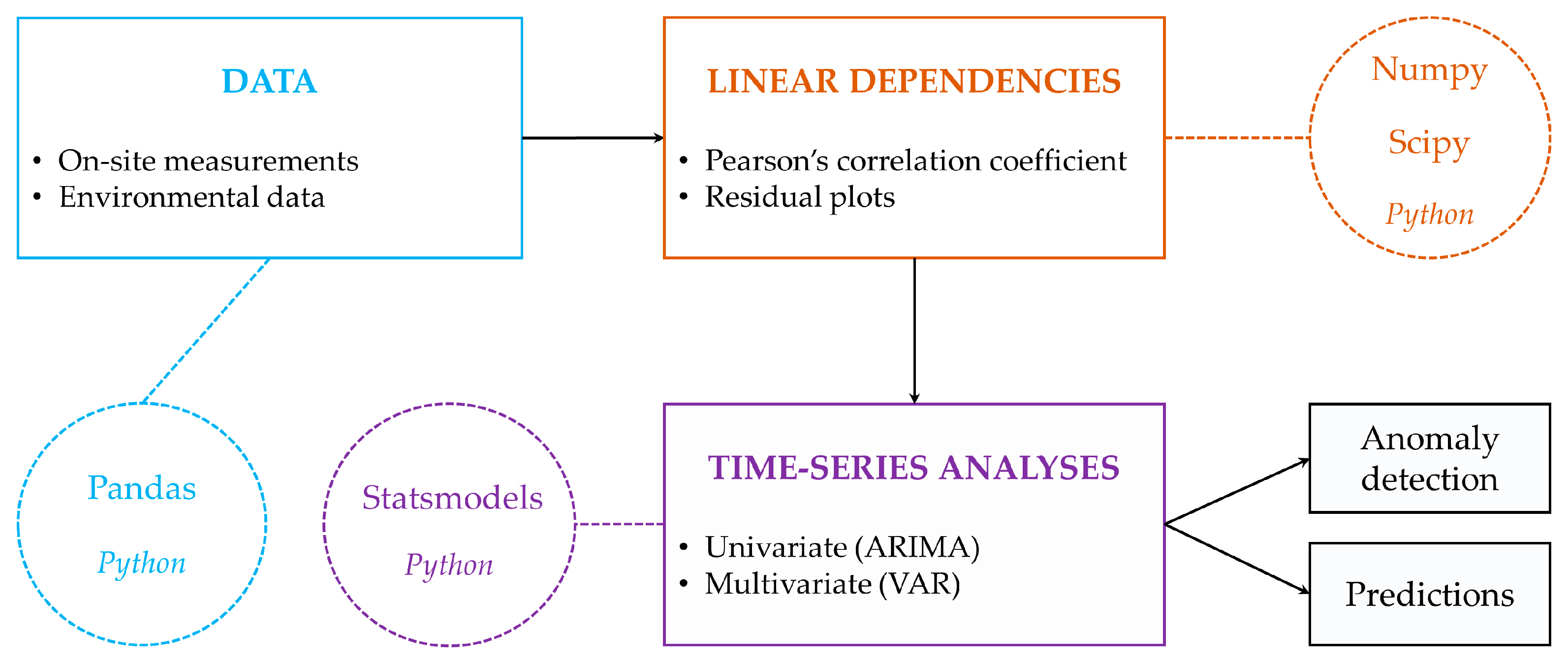
Python programming language and Python-based open-source libraries for data analysis were used in the study: Pandas—a data analysis library built on Python for handling tabulated data; NumPy and SciPy—libraries for scientific computing; Seaborn and Matplotlib—libraries for data visualization; Statsmodels—a module for exploring and modelling statistical data.
The analysis pipeline included the following steps. (i) Since the initial data of all variables used for the study (DO, river temperature, water level, sunshine duration, precipitation, and air temperature) were in tabular form, the Python-based library Pandas [17] was used to process the tabular data. (ii) Once the data were ready for further processing, we first investigated the linear dependence of the different parameters using the Python-based libraries Numpy [18] and Scipy [19] for scientific computing. At this stage, regression-based analyses were performed using Pearson’s correlation coefficient [20] as an indicator of linear dependence. (iii) Univariate and multivariate time series analyses based on autoregressive methods such as autoregressive integrated moving average (ARIMA) and vector autoregression model (VAR) were performed using Python-based Statsmodels module [21]. (iv) The Python-based plotting libraries Matplotlib [22] and Seaborn [23] were used to visualize the data (Figure 2).

3. Results and Discussion

3.1. Environmental Conditions in the Pivka River

Organic pollution from unknown sources, associated with low DO levels, was observed in the Pivka River during May 2016 (unpublished data). This event prompted the installation of an oxygen datalogger in the river upstream of where it sinks into Postojnska jama; this would facilitate the investigation of DO variations during the summer, a critical part of the year, usually with low river discharge and DO values. The logger was placed at the point immediately above where the river sinks into the karst underground, in order to obtain data concerning the input water conditions as applicable to the wellbeing of the groundwater biota. Despite there being evidence of relatively robust physiological adaptation of groundwater fauna to low DO [5], it is important to monitor the DO status at the ponor because aeration is virtually negligible when the river discharge is low and, in the absence of light, photosynthesis cannot take place to provide supplemental oxygen to the cave ecosystem.
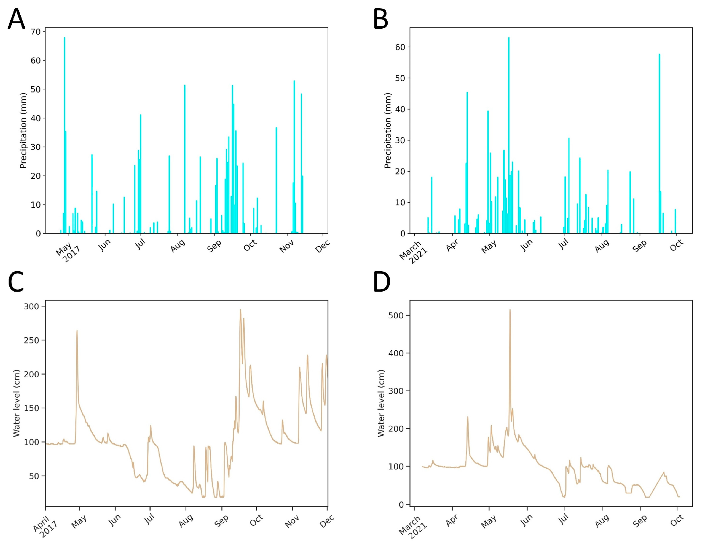
Records of two periods exhibiting different amounts of precipitation were analysed, with 2017 having about 24% less precipitation during the spring–autumn period compared to 2021 (Figure 3). For example, considering the same specific period, 846 mm of precipitation was recorded in the period 24 April–2 October in 2017, and 646 mm was recorded in 2021.
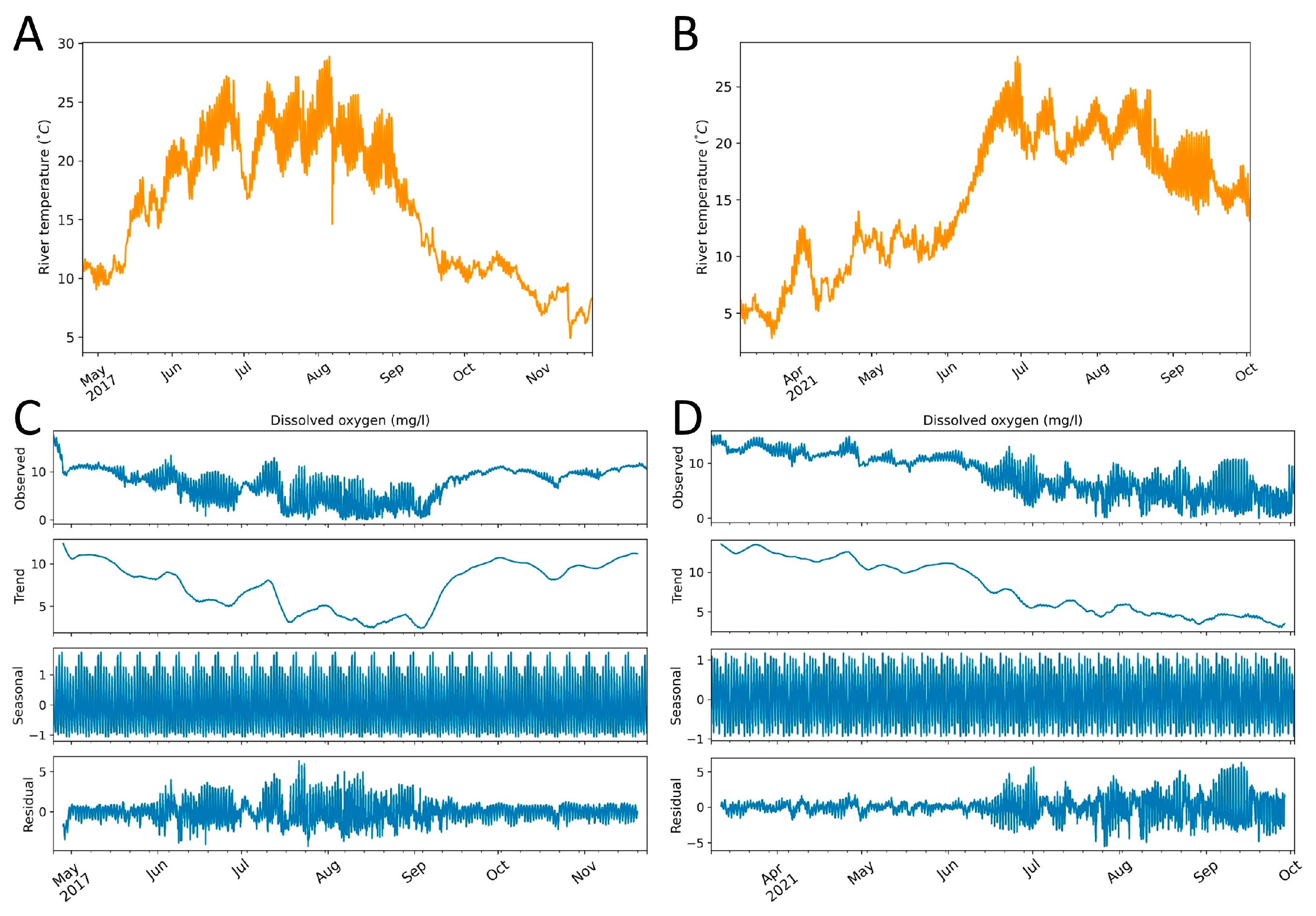
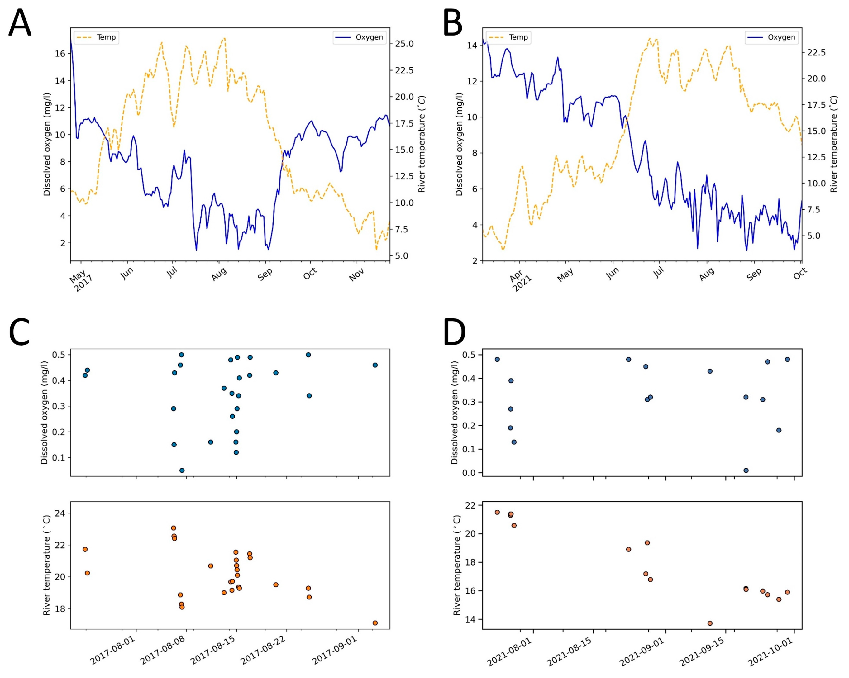
Temperature variations and corresponding DO levels of the Pivka River displayed different patterns during equivalent periods in 2017 and 2021 (Figure 4 and Figure 5). For example, from 24 April to 2 October 2017, the average temperature was 18.3 °C, and the corresponding average DO level was 6.80 mg/L; during the same period in 2021, the average temperature was 17.3 °C, and the related average DO value was 6.87 mg/L. Increases in temperature above 15 °C were accompanied by a rapid decrease in the DO levels from a concentration of about 10 mg/L (Figure 5). To understand the underlying pattern of the DO time-series data, the time series were decomposed into several components where T t , S t , R t denote trend, seasonality, and random error/residual, respectively (Equation (1)).
y t = T t + S t + R t
Trend refers to systematic changes in time series that represent a long-term direction. Seasonality refers to a repeating pattern of increasing and decreasing values that occurs consistently within the series throughout its duration. The random component represents statistical noise and is analogous to the error terms that are included in various types of statistical models, and it represents the remaining variation within a time series after trend and seasonality have been partitioned out (Figure 4).
The residual component showed relatively stable variation compared to large variations between July and August for the 2017 data and from July for the 2021 data. The large residual components suggested that the results of applying this simple decomposition approach neither helped to understand the underlying patterns of the data variations nor to replicate them, and that further analysis was required.
Because the rate of data acquisition was set to every 15 min to ensure the capture of any potential trend, the use of the daily mean of the measured DO data was also considered, to lessen the impact of any stochastic noise that might be present due to the high frequency data collection interval (Figure 5). The daily mean is an average of the 96 values recorded when data are collected at 15 min intervals for 24 h, i.e., i = 0 96 x i 96 .
Anoxic conditions were assumed to be those below a threshold DO value of 0.5 mg/L and, based upon this assumption, the datalogger obtained 130 and 76 readings for 2017 and 2021, respectively. To provide a clearer illustration, every fifth data point, starting with the first, was plotted, resulting in 26 points for 2017 and 16 points for 2021 (Figure 5C,D).

3.2. Relations between River Conditions and Atmospheric Parameters

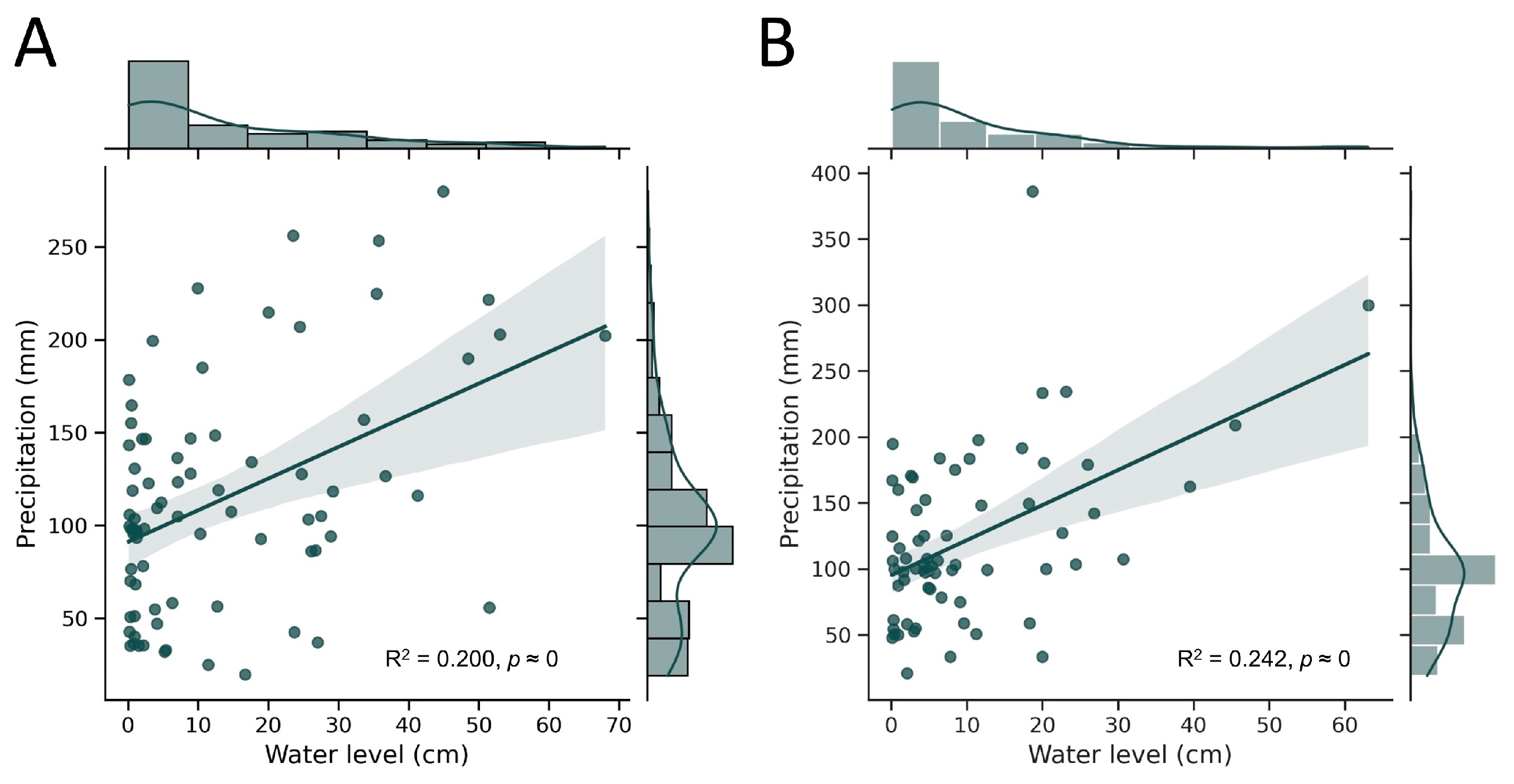
Publicly available hydrological and meteorological data were used in the following analyses, and related to on-site measurements of the DO and temperature within the Pivka River. Data on the amount of precipitation (re-sampled as a weekly median) and the river’s water level showed a linear correlation (Figure 6).
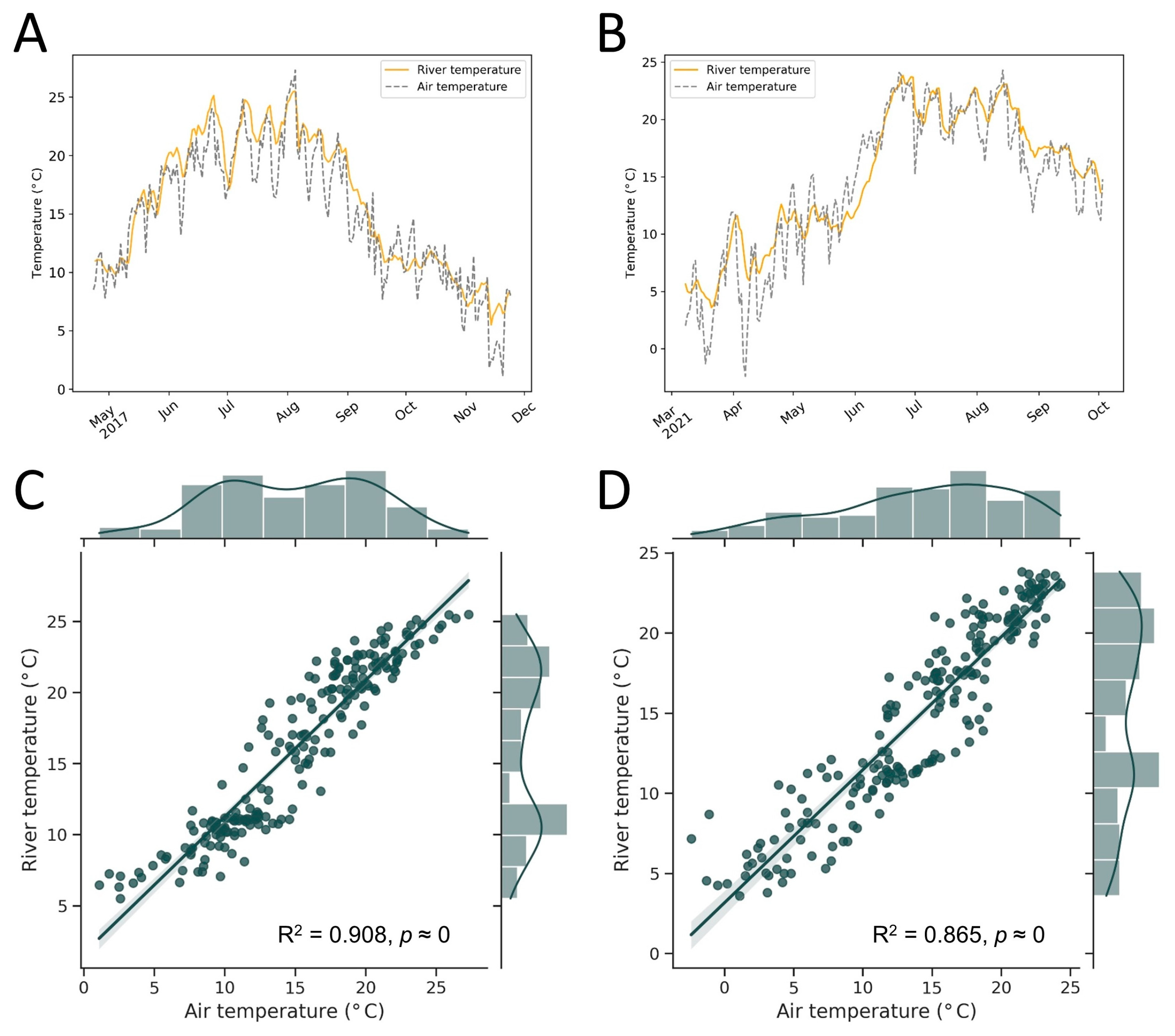
The air and river temperatures showed a linear relationship (Figure 7). This indicates that changes in water temperature reflect the changes in air temperature moderately well, and can be explained by the heat exchange between the water surface and the atmosphere. The Pearson correlation coefficient (r) indicates a high linear interdependence between water and air temperature (r = 0.953 for 2017, r = 0.930 for 2021).
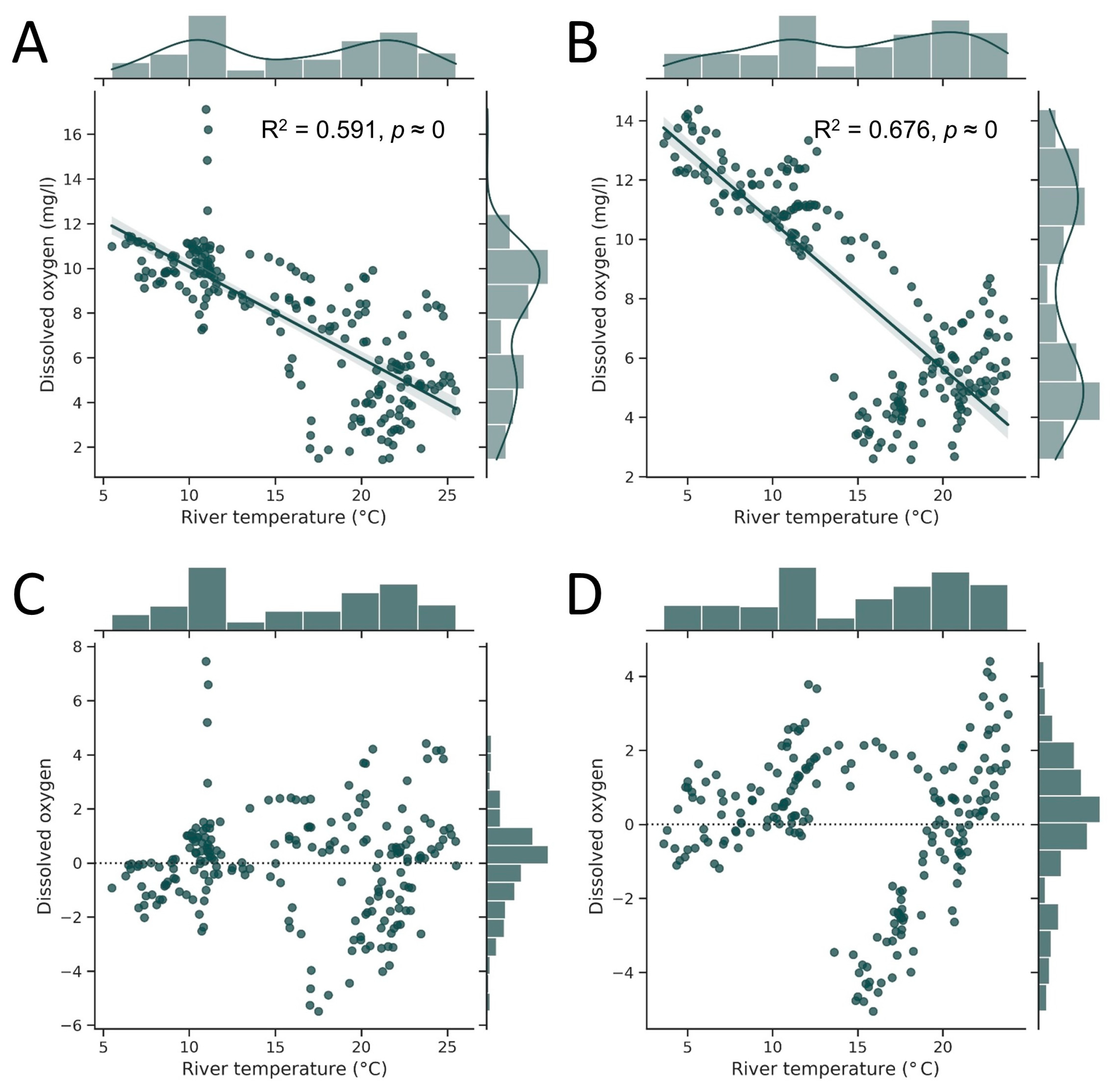
The increase in temperature associated with the decrease in DO is shown on the regression plot (for 2017: r = −0.769, p < 0.05; for 2021: r = −0.822, p < 0.05), but the residual plot showed that the residuals were not distributed evenly around the zero, suggesting that water temperature alone cannot account for the DO variation in the river (Figure 8).
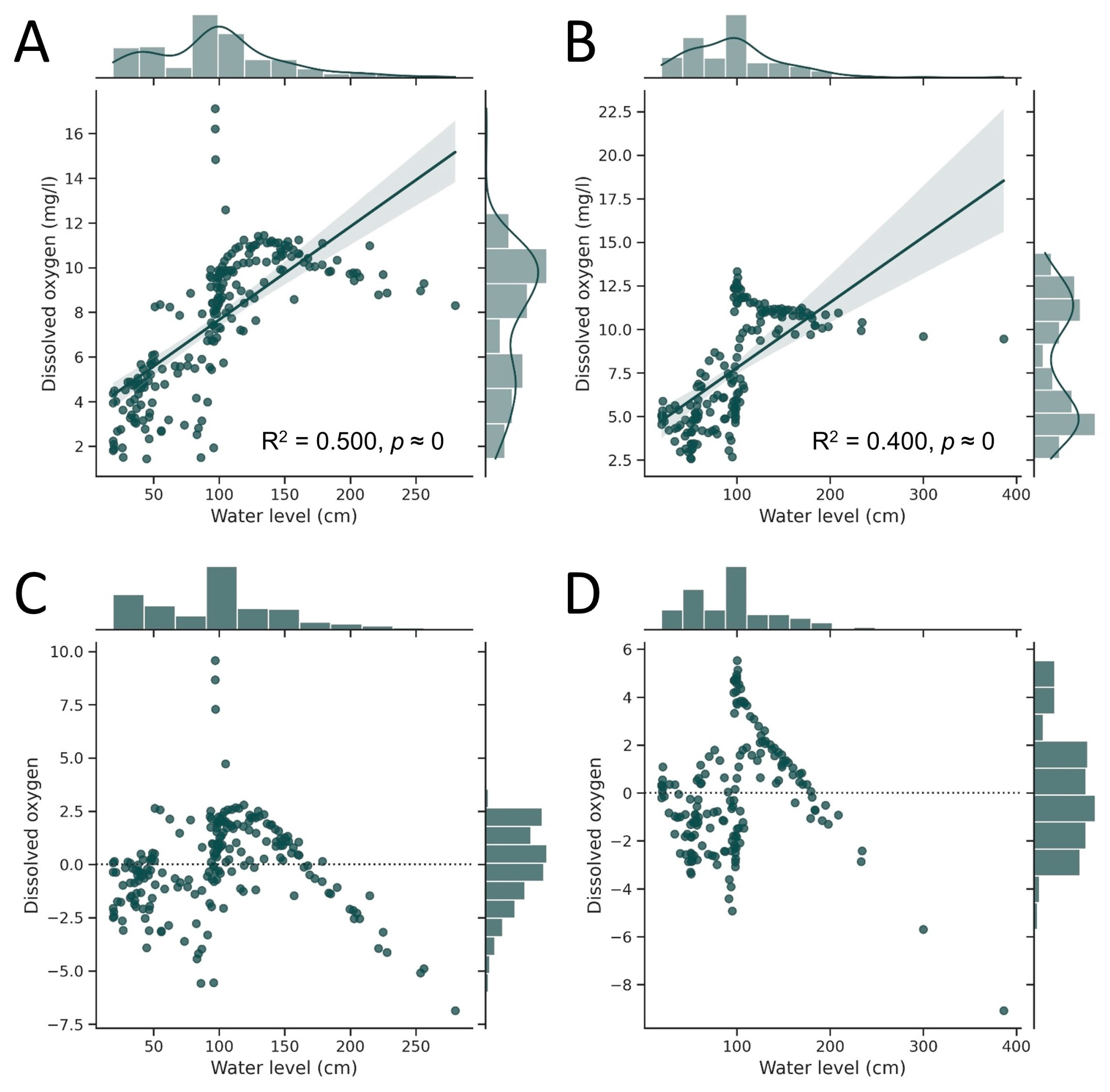
The water level in the Pivka River was related to the DO value, but the residual plot showed clearly that there was no linear correlation (for 2017: r = 0.71; for 2021: r = 0.63) (Figure 9). This is also confirmed by a scarcely noticeable relationship between the input of precipitation to the river and the DO level (Figure 10). It seems likely that the precipitation-related input pulse introduces water that is already oxygen depleted.
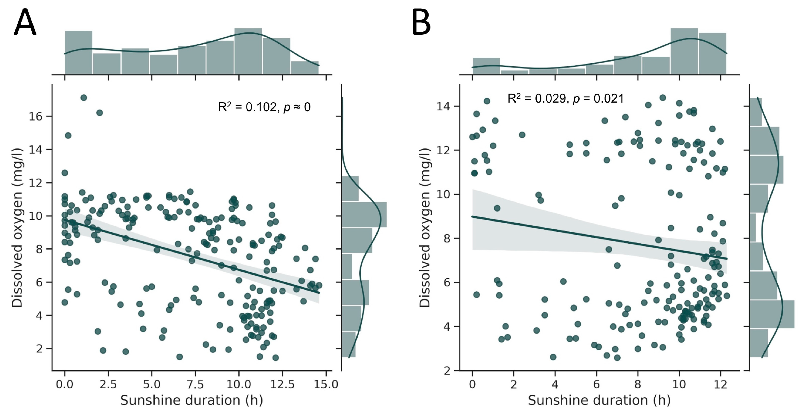
Oxygen is produced during the daylight phase of photosynthesis, so a positive correlation between hours of sunshine and DO might be expected, but this was not the case (Figure 11). At the studied site, oxygen consumption predominated over oxygen production, which might be partly due to there being suboptimal conditions for photosynthesis, because the monitoring site is located within the shaded area of the cave ponor (Figure 1).

3.3. Time-Series Analyses

Analysis of the temporal DO variations, utilized the univariate time-series model, comparing past data points and current oxygen readings to the current time-step. This differs from the multivariate time-series analysis discussed in the text below, which attempts to deduce an understanding of the DO changes by referencing to movements in the current or past values of measured DO and temperature.
Initially, a simple sliding window technique was applied to highlight any anomalies within the DO dataset. This technique is based upon predicting variations in subsequent time steps by using information about previous time steps. The number of previous time steps can also be referred to as a window. A sliding window was defined (one day consists of 96 data points) and repeatedly shifted towards the right until the end of the dataset. Mean (µ) and standard deviation (σ) values were computed within each window, and a local threshold was imposed. If a measured data point was less than µ − 2σ, it was considered an anomaly. Because the focus was on detecting low DO levels as anomalies, data points greater than µ + 2σ were not highlighted. Low DO values (0.05–0.23 mg/L) were measured between 24 July and 16 August 2017, and between 23 July and 27 September 2021. The total number of anomalous points found in 2017 was 40, with 8 distinct dates (24 July, 6 August, 7 August, 11 August, 13 August, 14 August, 15 August, 16 August), and for 2021 the number of anomalous points was 67, with 13 distinct dates (23 July, 26 July, 27 July, 8 August, 26 August, 27 August, 28 August, 11 September, 19 September, 23 September, 24 September, 25 September, 27 September) (Figure 12).
Subsequently, the ARIMA model [24] was performed on the datasets. The definition of the ARIMA model with parameters (p, d, q) is as follows (Equation (2))
ϕ p B 1 B d Y t = θ q B ϵ t
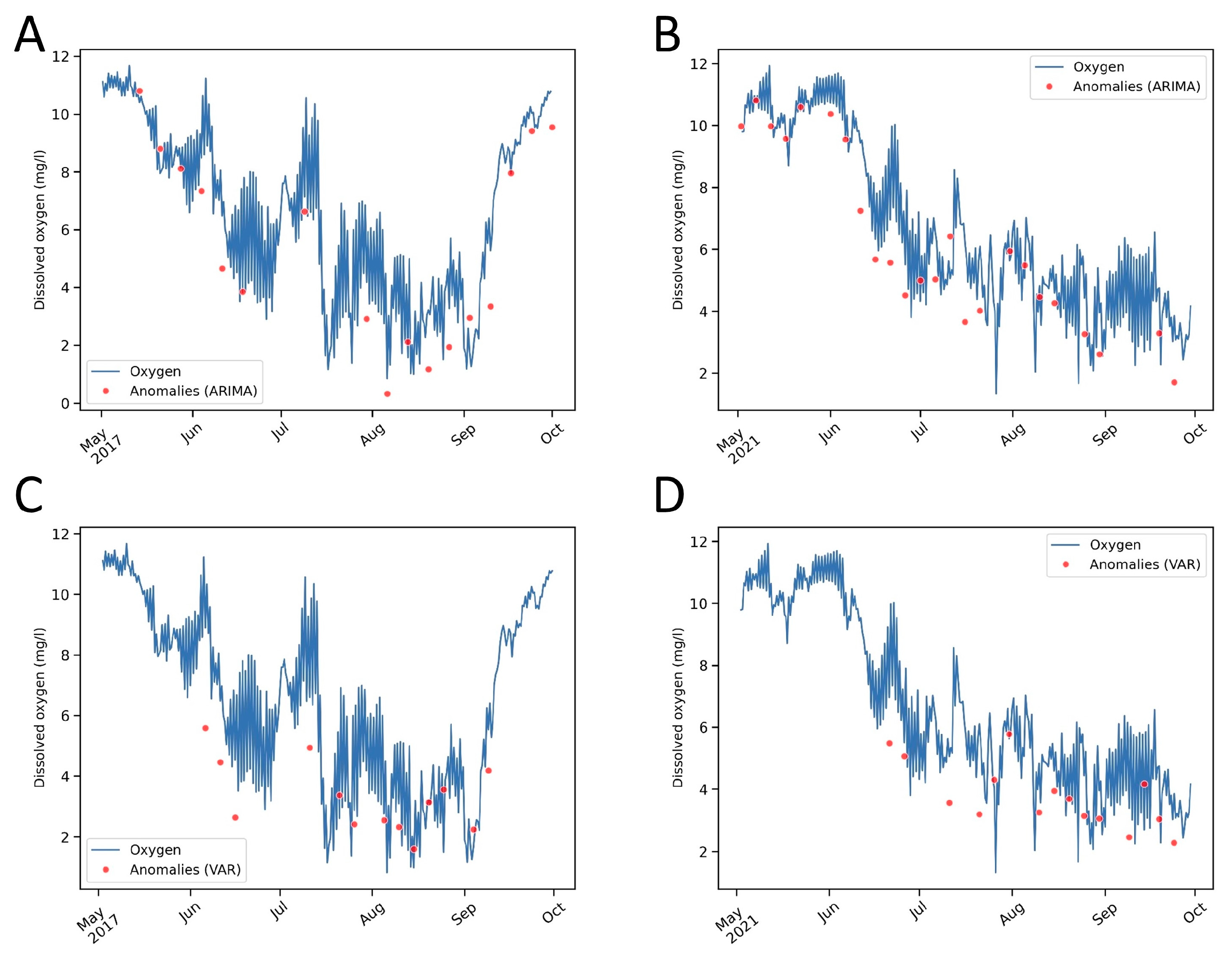
where the backshift operator B is defined as B p X t = X t p ,   ϕ i and θ i are the autoregressive (AR) and moving average (MA) parameters to be estimated, and ϵ i s are the series of residuals that are assumed to follow a normal distribution. The ARIMA model with (p, 0, 0) is the AR model, and with (0, 0, q), it is the MA model, and the integer d controls the level of differentiation. The AR and MA orders (p, q) were determined from autocorrelation function (ACF) and partial autocorrelation function (PACF) plots using the stationary time series. The augmented Dicky Fuller test (ADF) [18,25] was performed to confirm that the oxygen data were nonstationary, and the first-order differencing scheme was used to make the data stationary. Using these stationary data, the AR and MA orders (p, q) were determined as p = 7 and q = 1. The anomaly points were then detected as 2σ from the best fit ARIMA model on the stationary data. Finally, the difference was added to the stationary data to retrieve the original data points and the detected anomalous points along with the original measurement over a 30 min interval. To gain better representation of the anomalous points, the actual data points were re-sampled based on the weekly mean to reduce the number of anomalous points on the plot. Again, for one day, there are 96 data points due to the data collection interval being set at 15 min (Figure 13). Compared to Figure 12, the anomalous data points were similar around August 2017, but more anomalous points were detected due to the more robust and complex ARIMA model compared to the simple sliding window approach. More specifically, 40 points were detected starting with the data collected on 24 July 2017 at 20:30 to 16 August 2017 at 20:30 for the sliding window approach. For the ARIMA model, the total number of points after weekly re-sampling was 17, and without re-sampling, the total number of anomalous points was 5712 (17 × 48 × 7) in the period from 1 May 2017 to 30 September 2017. Consideration of the same time interval for the 2021 data resulted in 24 points after weekly re-sampling, and without re-sampling, the total number of anomalous points was 8064 (24 × 48 × 7).
Multivariate time-series analysis was applied to understand the effect of the relationship between the two data series, DO and temperature, either to confirm and/or possibly improve the detection of anomalies within a series by using not only the past information from a single time series (DO), but also additional information from the other series (in this case, temperature). The vector autoregression model (VAR) is one of the most commonly used models for multivariate time-series analysis [26]. The VAR model describes the time evolution of a set of endogenous variables Y t = y 1 t , y 2 t , , y n t with lag p as follows (Equation (3))
Y t = Π 1 Y t 1 + Π 2 Y t 2 + + Π p Y t p + ϵ t
where each time period is numbered t = 1 , , T ,   and ϵ t is an unobservable zero mean white noise vector process with a time-invariant covariance matrix Σ . An example of simplified bivariate scenario of the above equation is presented below (Equation (4))
y 1 t y 2 t = π 11 1 π 12 1 π 21 1 π 22 1 y 1 t 1 y 2 t 1 + π 11 2 π 12 2 π 21 2 π 22 2 y 1 t 2 y 2 t 2 + ϵ 1 t ϵ 2 t
The Statsmodels module was used to implement VAR, and the data analysis pipeline followed similar steps to those using the ARIMA model. The best lag p was found using minimum Akaike information criterion, AIC [27], and was p = 7.
The results of multivariate time-series anomaly detection with the VAR model in the May to September periods for the 2017 and 2021 data showed very similar results, i.e., detected anomalous points and their positions, as those of univariate anomaly detection with ARIMA. Focussing on the 2017 DO dataset, no such anomalous points were detected after the first week of September (approaching October) using the VAR model compared to the ARIMA analysis. This clearly indicates the temperature dependence of DO, where a decrease in temperature leads to an increase in DO in the water. However, in 2021, as the temperature started to decrease after September, DO did not increase (Figure 5). This could explain the anomalies observed in 2021, with both methods (ARIMA and VAR) applied to the analysis of the October measurements.
Independent oxygen time-series analysis and multivariate time-series analysis with dependence of oxygen and temperature found anomalous data points during a period when the DO levels fell below 3 mg/L.

3.4. Predictions and Perspectives

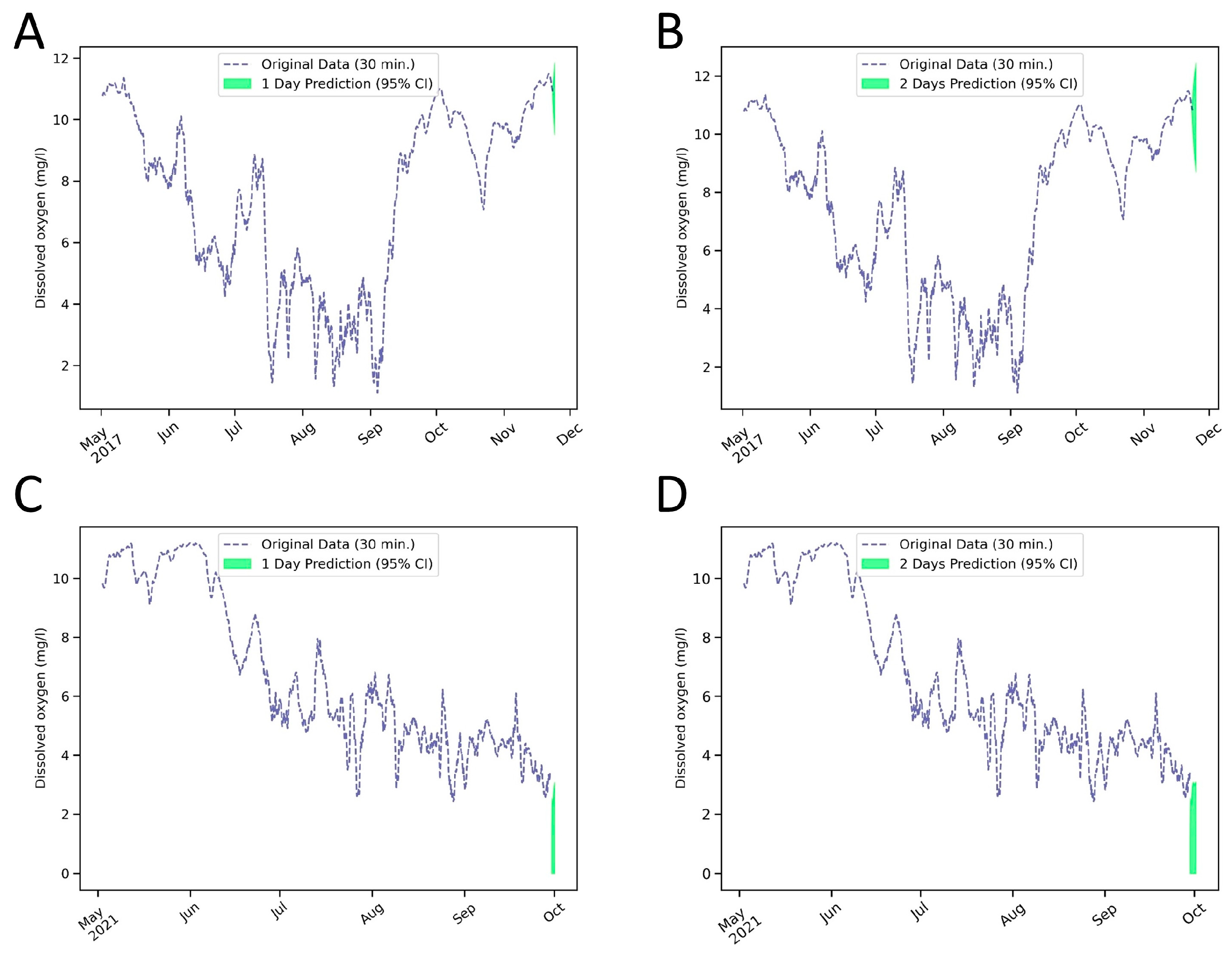
Modelling future dynamic trends based on large datasets for aquatic ecosystems is of increasing interest and importance to scientists, especially in relation to climatic changes [28]. The main objective of this study was to develop a robust analysis pipeline to support the identification of anomalous DO values based upon the measured data. The same model can also be used to predict future data points and identify potentially anomalous DO values. To demonstrate this, the ARIMA model was applied to data points with a 95% confidence interval (CI) (from 1 May to 23 November 2017; from 1 May to 29 September 2021) and predicted 1-day (96 data points) and 2-day concentrations of DO. It is important to note that during 2021, which was a dry year, the DO level in the river showed no increasing trend, and the levels predicted were even lower than the actual measured values (Figure 14).
Such intriguing results serve to direct future work on these data based on deep-learning approaches. Because the original data acquisition interval was 15 min, 2-day predictions require more than 192 points; at this point, models such as ARIMA and VAR would be too simplistic to predict many future points for complicated DO variations. Here, it is demonstrated that anomaly detection models could be used to obtain a rough estimate for a limited period, e.g., 1 day. Anomaly detection from previously obtained data is inherently different from future prediction, which depends upon several other parameters and requires robust analysis that will be addressed in the future using deep neural networks. The prediction of DO concentration for aquatic ecosystems on the basis of time-series analysis and deep learning is a challenging task for the future, but with the proper model, predictions are possible and can be reliable, even when only small datasets are available [29].
Whereas groundwater faunas exhibit some resilience and can tolerate anoxia for short periods [5,6], prolonged low DO levels present a risk that such conditions could persist for longer due to low discharge, lack of aeration and absence of photosynthesis in the complete darkness underground. The main parameters directing cycles of DO level are temperature, re-aeration, photosynthesis, light intensity, algal density, and respiration by any resident biotas [30]. In the case of organic pollution of a lake (comparable to the system during low or zero water discharge described above), its ecosystem slowly re-establishes the original, pre-pollution DO conditions. Changes in the DO pattern can be a clear indication of organic pollution [8]. Several anomalous events related to summer DO values were detected in the Pivka River. Whereas no major pollution events were recorded during the studied period, the possible occurrence of some minor local pollution events cannot be ruled out, such as seasonal fertilization from nearby agricultural fields and point pollution from illegal waste dumping. Not only direct anthropogenic pollution, but also extreme climatic conditions present challenges to the ecosystem. Supply of additional oxygenated water during extreme drought, when the DO level is low, seems to offer a possible remedy, but if this introduces alien biota into such vulnerable ecosystems, it is not acceptable. Ideally, future monitoring should include building a monitoring network by placing more DO loggers in the vertical profile to monitor the formation of oxygen stratification, and upstream in the riverbed to locate critical points of eutrophication. The use of additional online probes, for pH, nitrate, chloride, etc., in conjunction with real-time data analysis and a prediction model, would provide clearer insight into ecosystem dynamics and warn of potential sources of pollution. However, monitoring of DO levels, with use of the proposed analysis pipeline, provides an excellent basis for detecting extreme conditions and informing conservation planning for diversity hotspots.

4. Conclusions

The environmental conditions of the Pivka River were reconstructed in combination with in situ measurements and publicly available data. Increasing river temperature above 15 °C in summer corresponded with a rapid decrease in DO from 10 mg/L. Time-series analyses were used to detect low anomalous DO data points found when the DO level was below 3 mg/L and reached anoxic conditions when the DO was < 0.5 mg/L. The detected anomalies in the datasets were attributed not only to environmental conditions, but also to biological factors, when consumption of DO by metabolically active heterotrophic microbiota exceeded replenishment due to phototrophic oxygen production. Increases in river water-level were generally not reflected in higher DO values, which may be attributed to a pulse of oxygen-depleted water upstream. Predictions for future DO values were made using stable residuals. If there were no consecutive anomalous data points within a day, it was concluded that the DO level would increase after reaching a low value. The described example of an analysis pipeline based on known and site-specific threshold values, is particularly important for diversity hotspots where DO monitoring and early warnings of oxygen depletion are needed. Such an approach is especially necessary when variations in and critical levels of DO are difficult to observe for aquatic biota. The present study does not provide comprehensive answers to the behavior of such a complex ecosystem because more data are needed. Sometimes, data collection is almost impossible at such sites with extremely large discharge variations. Future steps, in addition to improving predictive models, should undoubtedly include the methodological approach, such as the use of technologies that allow direct data transmission in real time, which is then coupled with the proposed or similar analysis pipeline, resulting in an immediate alert when significant changes are detected. Such an approach could be applied not only to the river ecosystems presented, but also to lakes and other artificial water bodies such as accumulation reservoirs for hydroelectric power plants.

Author Contributions

J.M. and A.O.-M. conceived and designed the experiment. S.B. performed statistical analyses. All authors wrote the paper. All authors have read and agreed to the published version of the manuscript.

Funding

This research received no external funding.

Institutional Review Board Statement

Not applicable.

Informed Consent Statement

Not applicable.

Data Availability Statement

The data presented in this study are openly available at GitHub (https://github.com/suvoooo/Cave-Analysis).

Acknowledgments

The authors acknowledge financial support from the Slovenian Research Agency (research core funding No. P6-0119 and P2-0412) and the monitoring plan for Postojnska jama. Our thanks also to Franjo Drole, Matej Blatnik, Ksenija Dvorščak and Metka Petrič for providing valuable support with field work and collection, and to David Lowe for assistance with English language editing.

Conflicts of Interest

The authors declare no conflict of interest. The founding sponsors had no role in the design of the study; in the collection, analyses, or interpretation of data; in the writing of the manuscript; or in the decision to publish the results.

References

  1. Yan, T.; Shen, S.L.; Zhou, A. Indices and models of surface water quality assessment: Review and perspectives. Environ. Pollut. 2022, 308, 119611. [Google Scholar] [CrossRef]
  2. Breitburg, D.; Levin, L.A.; Oschlies, A.; Grégoire, M.; Chavez, F.P.; Conley, D.J.; Garçon, V.; Gilbert, D.; Gutiérrez, D.; Isensee, K.; et al. Declining oxygen in the global ocean and coastal waters. Science 2018, 359, eaam7240. [Google Scholar] [CrossRef] [PubMed] [Green Version]
  3. Wurtsbaugh, W.; Paerl, H.; Dodds, W. Nutrients, eutrophication and harmful algal blooms along the freshwater to marine continuum. Wiley Interdiscip. Rev. Water 2019, 6, e1373. [Google Scholar] [CrossRef]
  4. Banti, V.; Giuntoli, B.; Gonzali, S.; Loreti, E.; Magneschi, L.; Novi, G.; Paparelli, E.; Parlanti, S.; Pucciariello, C.; Santaniello, A.; et al. Low oxygen response mechanisms in green organisms. Int. J. Mol. Sci. 2013, 14, 4734–4761. [Google Scholar] [CrossRef] [PubMed] [Green Version]
  5. Malard, F.; Hervant, F. Oxygen supply and the adaptations of animals in groundwater. Freshw. Biol. 1999, 41, 1–30. [Google Scholar] [CrossRef]
  6. Issartel, J.; Hervant, F.; de Fraipont, M.; Clobert, J.; Voituron, Y. High anoxia tolerance in the subterranean salamander Proteus anguinus without oxidative stress nor activation of antioxidant defenses during reoxygenation. J. Comp. Physiol. B Biochem. Syst. Environ. Physiol. 2009, 179, 543–551. [Google Scholar] [CrossRef] [PubMed]
  7. García, H.; Gordon, L. Oxygen solubility in seawater—Better fitting equations. Limnol. Oceanogr. 1992, 37, 1307–1312. [Google Scholar] [CrossRef]
  8. Ansa-Asare, O.; Marr, I.; Cresser, M. Evaluation of modelled and measured patterns of dissolved oxygen in a freshwater lake as an indicator of the presence of biodegradable organic pollution. Water Res. 2000, 34, 1079–1088. [Google Scholar] [CrossRef]
  9. Culver, D.; Sket, B. Hotspots of subterranean biodiversity in caves and wells. J. Cave Karst Stud. 2000, 62, 11–17. [Google Scholar]
  10. Zagmajster, M.; Polak, S.; Fišer, C. Postojna-Planina cave system in Slovenia, a hotspot of subterranean biodiversity and a cradle of speleobiology. Diversity 2021, 13, 271. [Google Scholar] [CrossRef]
  11. Cox, B. A review of currently available in-stream water-quality models and their applicability for simulating dissolved oxygen in lowland rivers. Sci. Total Environ. 2003, 314, 335–377. [Google Scholar] [CrossRef] [PubMed]
  12. Elkiran, G.; Nourani, V.; Abba, S.I.; Abdullahi, J. Artificial intelligence-based approaches for multi-station modelling of dissolve oxygen in river. Glob. J. Environ. Sci. Manag. 2018, 4, 439–450. [Google Scholar] [CrossRef]
  13. Banerjee, A.; Chakrabarty, M.; Rakshit, N.; Bhowmick, A.; Ray, S. Environmental factors as indicators of dissolved oxygen concentration and zooplankton abundance: Deep learning versus traditional regression approach. Ecol. Indic. 2019, 100, 99–117. [Google Scholar] [CrossRef]
  14. Ouma, Y.; Okuku, C.; Njau, E. Use of artificial neural networks and multiple linear regression model for the prediction of dissolved oxygen in rivers: Case study of hydrographic basin of River Nyando, Kenya. Complexity 2020, 2020, 9570789. [Google Scholar] [CrossRef]
  15. Buser, S.; Grad, K.; Pleničar, M. Basic Geological Map of SFRY 1:100.000, Sheet Postojna; Federal Geological Survey: Belgrade, Yugoslavia, 1967. [Google Scholar]
  16. Mulec, J.; Petrič, M.; Koželj, A.; Brun, C.; Batagelj, E.; Hladnik, A.; Holko, L. A multiparameter analysis of environmental gradients related to hydrological conditions in a binary karst system (underground course of the Pivka River, Slovenia). Acta Carsol. 2019, 48, 313–327. [Google Scholar] [CrossRef]
  17. McKinney, W. Data structures for statistical computing in python. In Proceedings of the 9th Python in Science Conference, Austin, TX, USA, 28 June–3 July 2010; Volume 445, pp. 51–56. [Google Scholar]
  18. Harris, C.R.; Millman, K.J.; Van Der Walt, S.J.; Gommers, R.; Virtanen, P.; Cournapeau, D.; Wieser, E.; Taylor, J.; Berg, S.; Smith, N.J.; et al. Array programming with NumPy. Nature 2020, 585, 357–362. [Google Scholar] [CrossRef]
  19. Virtanen, P.; Gommers, R.; Oliphant, T.E.; Haberland, M.; Reddy, T.; Cournapeau, D.; Burovski, E.; Peterson, P.; Weckesser, W.; Bright, J.; et al. SciPy 1.0: Fundamental algorithms for scientific computing in Python. Nat. Methods 2020, 17, 261–272. [Google Scholar] [CrossRef] [PubMed] [Green Version]
  20. Pearson, K. VII. Note on regression and inheritance in the case of two parents. Proc. R. Soc. Lond. 1895, 58, 240–242. [Google Scholar]
  21. Seabold, S.; Perktold, J. Statsmodels: Econometric and statistical modeling with python. In Proceedings of the 9th Python in Science Conference, Austin, TX, USA, 28 June–3 July 2010; Volume 57, pp. 92–96. [Google Scholar]
  22. Hunter, J.D. Matplotlib: A 2D graphics environment. Comput. Sci. Eng. 2007, 9, 90–95. [Google Scholar] [CrossRef]
  23. Waskom, M.L. Seaborn: Statistical data visualization. J. Open Source Softw. 2021, 6, 3021. [Google Scholar] [CrossRef]
  24. Millis, T.C. A Very British Affair: Six Britons and the Development of Time Series Analysis during the 20th Century; Palgrave Macmillan: London, UK, 2013; pp. 161–215. [Google Scholar]
  25. Dickey, D.; Fuller, W. Distribution of the estimators for autoregressive time series with a unit root. J. Am. Stat. Assoc. 1979, 74, 427–431. [Google Scholar] [CrossRef]
  26. Lütkepohl, H. New Introduction to Multiple Time Series Analysis; Springer Science & Business Media: Berlin, Germany, 2005; p. 764. [Google Scholar]
  27. Akaike, H. A new look at the statistical model identification. IEEE Trans. Autom. Contr. 1974, 19, 716–723. [Google Scholar] [CrossRef]
  28. Zhu, S.; Bonacci, O.; Oskoru, D.; Hadzima-Nyarko, M.; Wu, S. Long term variations of river temperature and the influence of air temperature and river discharge: Case study of Kupa River watershed in Croatia. J. Hydrol. Hydromech. 2019, 67, 305–313. [Google Scholar] [CrossRef] [Green Version]
  29. Zhu, N.; Ji, X.; Tan, J.; Jiang, Y.; Guo, Y. Prediction of dissolved oxygen concentration in aquatic systems based on transfer learning. Comput. Electron. Agric. 2021, 180, 105888. [Google Scholar] [CrossRef]
  30. Portielje, R.; Lijklema, L. The effect of reaeration and benthic algae on the oxygen balance of an artificial ditch. Ecol. Modell. 1995, 79, 35–48. [Google Scholar] [CrossRef]
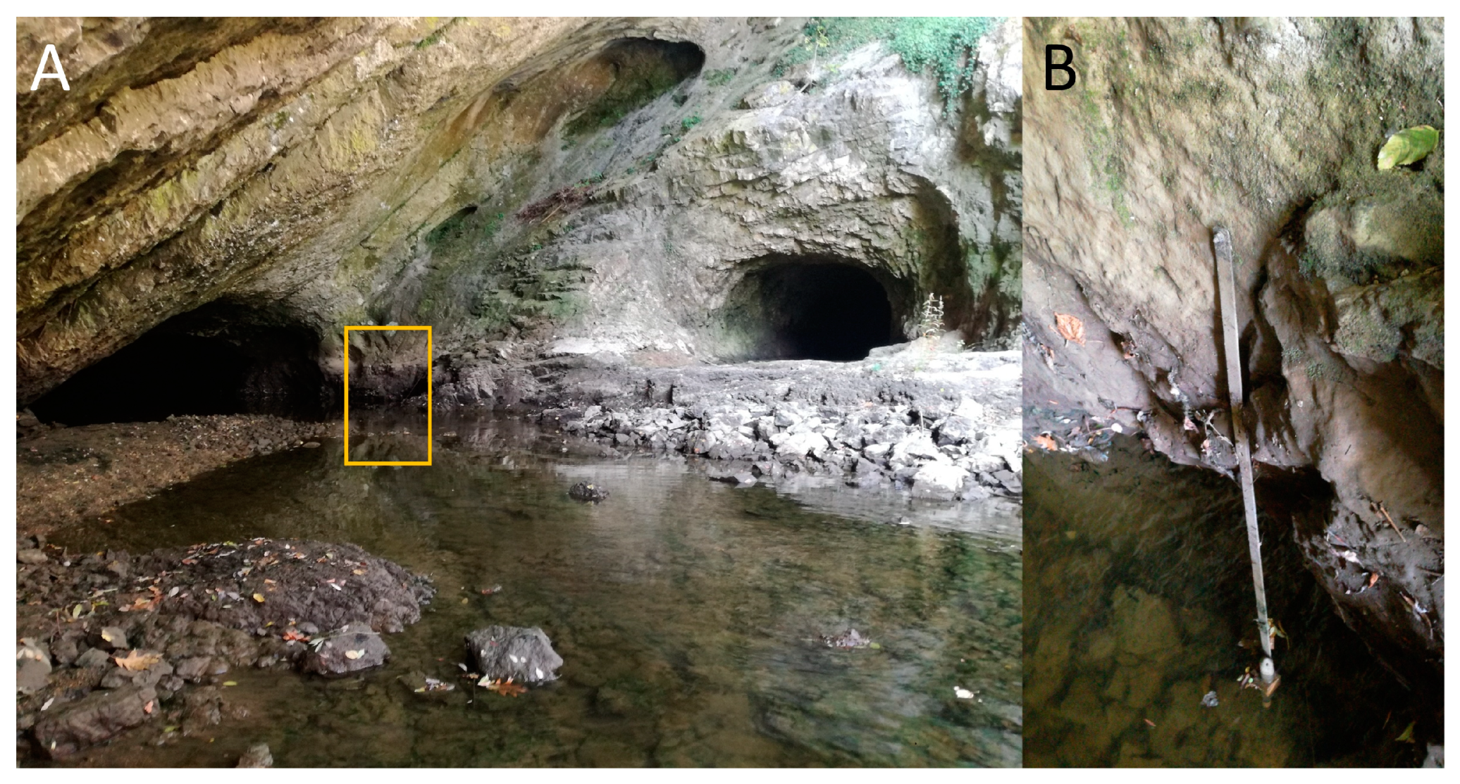
Figure 1. The Pivka River above its sink into Postojnska jama: (A) view of the ponor under extremely low water-level conditions, yellow box showing the designated position of the datalogger; (B) datalogger on site (4 October 2021).
Diversity 15 00156 g001
Figure 2. Data analysis pipeline with analysis tools used in the study. The square blocks represent the analysis steps and the circles represent the analysis tools.
Diversity 15 00156 g002
Figure 3. (A,B) Precipitation and (C,D) water level of the Pivka River in spring–autumn in 2017 and 2021, respectively.
Diversity 15 00156 g003
Figure 4. (A,B) River temperature and (C,D) DO in the river as measured (observed) and with additive time-series decomposition for variation of oxygen (trend, seasonal, residual) in 2017 and 2021, respectively. The measured data are assumed to be the sum of the trend, seasonality and residuals.
Diversity 15 00156 g004
Figure 5. (A,B) DO data re-sampled as daily mean and (C,D) data points for DO < 0.5 mg/L and temperature of every 5th data point in 2017 and 2021, respectively.
Diversity 15 00156 g005
Figure 6. (A,B) Relationships between the water level of the Pivka River (measured daily) and precipitation on a regression plot in 2017 and 2021, respectively.
Diversity 15 00156 g006
Figure 7. (A,B) Air temperature recorded by the ARSO meteorological station at Postojna and the water temperature in the Pivka River and (C,D) temperature regression plot in 2017 and 2021, respectively.
Diversity 15 00156 g007
Figure 8. (A,B) Regression plot of temperature and DO of the Pivka River and (C,D) residual plot in 2017 and 2021, respectively.
Diversity 15 00156 g008
Figure 9. (A,B) Regression plot of water level and DO of the Pivka River and (C,D) residual plot in 2017 and 2021, respectively.
Diversity 15 00156 g009
Figure 10. (A,B) Regression plot of precipitation and DO in 2017 and 2021, respectively.
Diversity 15 00156 g010
Figure 11. (A,B) Regression plot of DO and sunshine duration in 2017 and 2021, respectively.
Diversity 15 00156 g011
Figure 12. Detection of anomalies in DO data using a simple sliding window approach with a 24 h window. Points were classified as anomalies (red dots), when the real data points were <µ − 2σ: (A) between 24 July and 16 August 2017; (B) between 23 July and 27 September 2021.
Diversity 15 00156 g012
Figure 13. Time-series analyses of measured DO levels with detected anomalous points re-sampled over a week (red dots): (A) ARIMA model for 2017 data; (B) ARIMA model for 2021 data; (C) VAR model for 2017 data; (D) VAR model for 2021 data.
Diversity 15 00156 g013
Figure 14. Prediction for future DO values based on an ARIMA model with 95% CI, shown as green range: (A) 1-day prediction based on the 2017 dataset; (B) 2-day prediction based on the 2017 dataset; (C) 1-day prediction based on the 2021 dataset; (D) 2-day prediction based on the 2021 dataset (some of the values predicted fell below 0 mg/L of DO, and for these values, a threshold was imposed at 0.00 mg/L).
Diversity 15 00156 g014
Disclaimer/Publisher’s Note: The statements, opinions and data contained in all publications are solely those of the individual author(s) and contributor(s) and not of MDPI and/or the editor(s). MDPI and/or the editor(s) disclaim responsibility for any injury to people or property resulting from any ideas, methods, instructions or products referred to in the content.