Article

Habitat Provision and Erosion Are Influenced by Seagrass Meadow Complexity: A Seascape Perspective

by
Giulia Ferretto
1,2,*,
Adriana Vergés
1,3,
Alistair G. B. Poore
1,3,
Tim M. Glasby
1,4 and
Kingsley J. Griffin
1,2
1
Centre for Marine Science and Innovation, School of Biological, Earth and Environmental Sciences, University of New South Wales, Sydney, NSW 2052, Australia
2
School of Biological Sciences & Oceans Institute, University of Western Australia, Perth, WA 6009, Australia
3
Sydney Institute of Marine Science, Mosman, NSW 2088, Australia
4
NSW Department of Primary Industries, Port Stephens Fisheries Institute, Port Stephens, NSW 2315, Australia
*
Author to whom correspondence should be addressed.
Diversity 2023, 15(2), 125; https://doi.org/10.3390/d15020125
Submission received: 18 November 2022 / Revised: 16 December 2022 / Accepted: 28 December 2022 / Published: 17 January 2023
(This article belongs to the Special Issue Seagrass Ecosystems, Associated Biodiversity, and Its Management)

Abstract

:
Habitat complexity plays a critical role in shaping biotic assemblages and ecosystem processes. While the impacts of large differences in habitat complexity are often well understood, we know less about how subtle differences in structure affect key ecosystem functions or properties such as biodiversity and biomass. The late-successional seagrass Posidonia australis creates vital habitat for diverse fauna in temperate Australia. Long-term human impacts have led to the decline of P. australis in some estuaries of eastern Australia, where it is now classified as an endangered ecological community. We examined the influence of P. australis structural complexity at small (seagrass density) and large (meadow fragmentation) spatial scales on fish and epifauna communities, predation and sediment erosion. Fine-scale spatially balanced sampling was evenly distributed across a suite of environmental covariates within six estuaries in eastern Australia using the Generalised Random Tessellation Structures approach. We found reduced erosion in areas with higher P. australis density, greater abundance of fish in more fragmented areas and higher fish richness in vegetated areas further from patch edges. The abundance of epifauna and fish, and fish species richness were higher in areas with lower seagrass density (seagrass density did not correlate with distance to patch edge). These findings can inform seagrass restoration efforts by identifying meadow characteristics that influence ecological functions and processes.

1. Introduction

Seascape habitat structure and complexity (hereafter referred to as habitat complexity) can strongly influence biotic assemblages, ecosystem functioning and processes [1]. For example, more complex habitats generally host higher richness and abundance of associated species because they provide a greater variety of niches [2]. Differences in habitat complexity can also influence predator-prey interactions [3,4], for example by altering availability of shelter for prey and access to predators [5].
Seascape habitat complexity incorporates small-scale structural complexity (e.g., shoot density of plants) and large-scale variables related to the spatial configuration and fragmentation of habitats [6]. Our understanding of how ecosystem functions and processes are impacted by different components of habitat complexity is limited and at times, conflicting. For example, several studies suggest fragmentation leads to declines in carbon stocks and biodiversity [7,8,9]. In contrast, Fahrig [10] reports positive effects of fragmentation ‘per se’ on biodiversity and habitat functioning.
The growth of human populations, overexploitation of natural resources and climate change are modifying ecosystems globally, increasing habitat degradation and unpredictably altering habitat complexity [11,12,13], resulting in impacts on biodiversity [14], ecosystem functioning [15,16] and ecosystems services [17,18,19]. The decline in foundation species (i.e., species that support biodiversity and define the structure of a community) can have dramatic consequences for habitat complexity and dependent species, leading to disproportionate effects on ecosystem functions [14,20,21].
Marine ecosystems are heavily impacted by human activities globally [11] and recent decades have seen extensive changes in the overall abundance and habitat complexity of habitats such as kelp forests [22] and seagrass meadows [23,24]. Seagrasses are marine flowering plants that form extensive coastal habitats that support high biodiversity and provide a range of ecosystem functions [25]. Some seagrasses can capture and store carbon more efficiently than terrestrial plants [26,27], create a dense habitat where a wide variety of fauna can live, find protection and/or forage [28,29], and they prevent coastal erosion by stabilising sediment [30]. Seagrass habitats support higher biodiversity and perform a range of ecosystem functions beyond unvegetated habitats [31,32,33] but we have limited information on how differences in habitat complexity are impacting these relationships.
Habitat complexity can influence the composition of seagrass associated macroinvertebrates [34] and fish [35,36,37], and impact ecological processes like predation [5]. This has been investigated by isolating individual aspects of habitat complexity, such as patch size and distance to meadow edge [32,38,39,40]. Fish assemblages across estuarine seascapes are also shaped by seagrass meadows [41] and by landscape patterns at different spatial scales, including habitat composition and configuration [42]. Differences in habitat complexity can alter sediment movement [30] for example by altering hydrodynamic flow at within-patch [43] and meadow scales [44]. However, our understanding of how seagrass habitat complexity at multiple spatial scales influences ecosystem functions is limited and having this information can guide conservation and restoration approaches.
In this study we examine how habitat complexity relates to ecosystem functions (fish and epifauna composition, predation and sediment erosion rates) at several spatial scales to inform conservation and restoration of the threatened seagrass, Posidonia australis (Hook.f.). This seagrass is endemic to the southern half of Australia, where it creates dense meadows in sheltered and shallow bays. Some economically important species of fish and invertebrates depend on P. australis complex habitat during their juvenile stages or during their whole life [45,46]. There is evidence that some fish species respond to small-scale differences in P. australis habitat complexity [47] and macrofauna abundance may be driven by habitat preference [48] but little is known about the consequences that differences in habitat complexity may have on seagrass-associated species assemblages.
Long-term human impacts have led to the decline of P. australis in some estuaries of eastern Australia. Six populations of P. australis in south-eastern Australia being listed as endangered under NSW Government legislation in 2012 (Fisheries Management Act 1994 (NSW), Australia) and an additional three estuaries were also listed as threatened ecological communities under the Commonwealth legislation in 2015 (Environment Protection and Biodiversity Conservation Act 1999 (Cth), Australia (EPBC Act)). Some populations are still declining despite protection [49,50], due to multiple impacts including boat moorings [51], dredging and construction [52]. P. australis can take decades to recover after disturbances due to slow growth rates [53]. Small-scale restoration projects using innovative techniques to revegetate areas where P. australis has declined are having success [54] but the challenge now, in the UN Decade of Ecosystem Restoration, is to scale-up restoration efforts [55]. Mitigation approaches such as conservation and restoration projects are becoming essential tools to reverse the decline of foundation species such as seagrasses. Thus, quantifying the relationships between habitat complexity and ecosystem functions better informs restoration strategies and outcomes (e.g., by helping select targets for restoration projects). This is particularly relevant for the recovery of ecological communities associated with endangered and slow-growing species like P. australis.
Working across six estuaries that include some of the most impacted P. australis meadows in south-eastern Australia, we quantify how habitat complexity (seagrass density, meadow fragmentation and distance to meadow edge) is related to: (1) fish abundance and species composition, (2) mobile epifauna abundance, (3) fish predation rates and (4) erosion rates. As marine fauna and processes can respond to complexity at different spatial scales [56], we used a seascape approach that incorporates variability at different levels including sub-patch (e.g., seagrass shoot scale; [57]), within-patch (e.g., distance to meadow edge; [40]) and among-patch (connectivity) or seascape scale [58]. Seascape ecology is a growing field of marine science that brings spatial approaches common in terrestrial landscape ecology into marine ecosystems to help resolve spatial patterns [59,60]. Including a seascape approach allows a deeper understanding of heterogenous marine ecosystems and their connections, incorporating the natural interconnectivity of seascapes, which are shaped by patterns and processes that operate at multiple spatial scales [6,59].

2. Materials and Methods

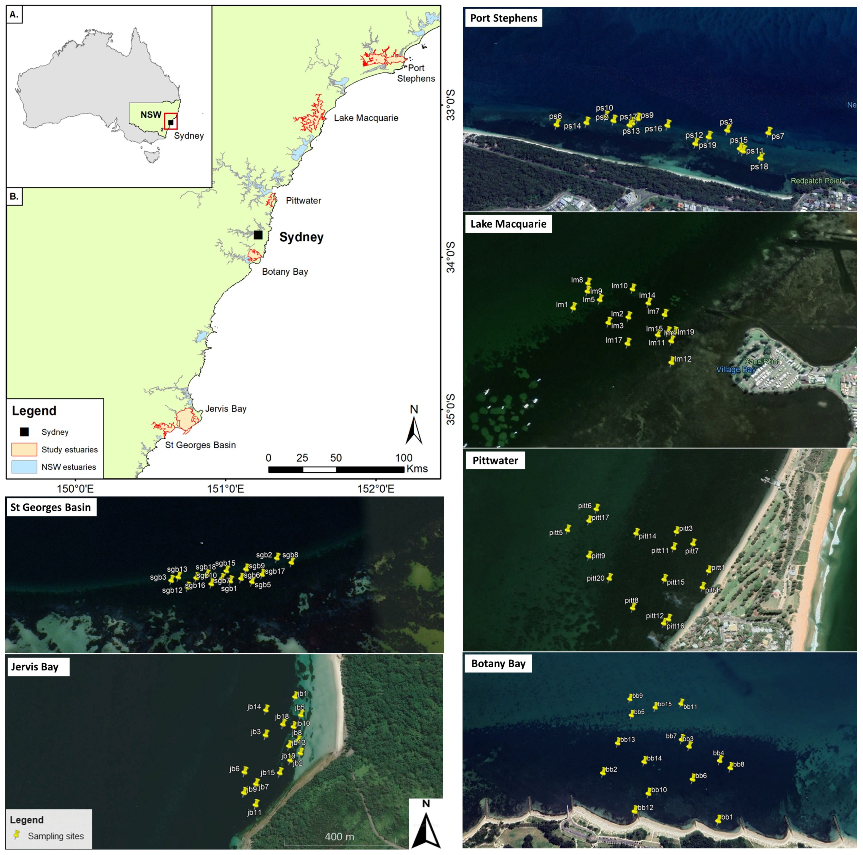
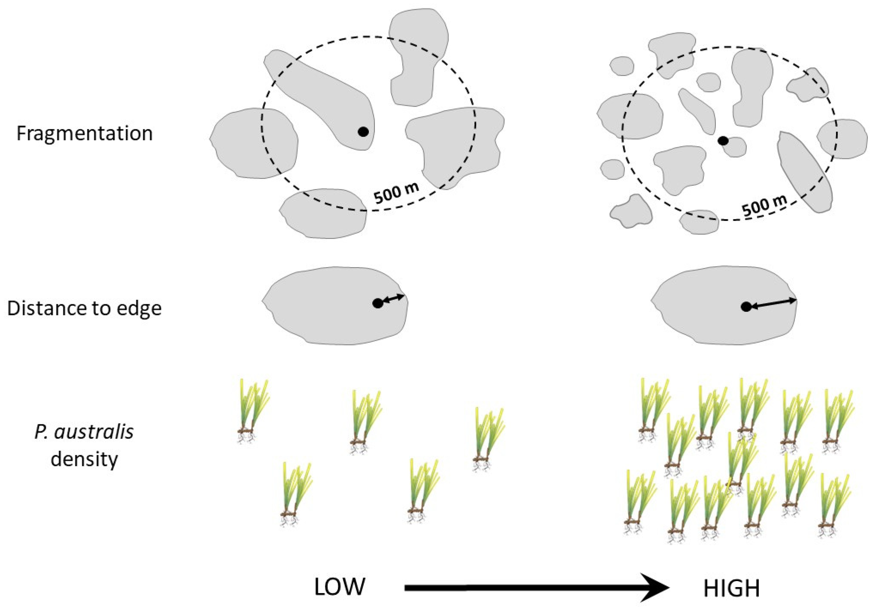
2.1. Study Estuaries and a-Priori Site Selection

Fish and epifauna composition, sediment erosion and predation rates were quantified in Posidonia australis meadows in six different estuaries in New South Wales, Australia (Figure 1). These included three estuaries in which P. australis is classified as endangered under the NSW and Commonwealth Government legislation: Lake Macquarie (−33.049637, 151.647302), Pittwater (−33.591091,151.318788) and Botany Bay (−34.006181, 151.193384), and three estuaries where P. australis is not endangered under NSW Government legislation: Port Stephens (−32.718373, 152.125055), Jervis Bay (−35.040582, 150.784482) and St Georges Basin (−35.140870, 150.638630; Figure 1). The P. australis ecological community in Port Stephens is listed as endangered under the Commonwealth legislation. P. australis is confined to only 17 of the 121 NSW estuaries known to contain seagrass [50] and only grows in three geomorphic types of estuaries, specifically ocean embayments (Botany Bay and Jervis Bay), tide-dominated estuaries (Port Stephens and Pittwater) and wave-dominated estuaries (Lake Macquarie and St Georges Basin) see [61] for details on the characterises of these estuaries. Although the six estuaries display some different environmental characteristics (Table S1), the sampled areas included here are characterised by broadly similar oceanographic regimes that enable Posidonia australis to occur, including high salinity, low nutrients levels and relatively stable environmental conditions [61].
P. australis distribution was initially identified using the high-quality imagery program NearMap Australia. High-resolution spatial layers describing the area and extent of P. australis were obtained using the latest available seagrass mapping in each estuary (NSW Fisheries Spatial Data Portal) [62]. We selected a single meadow within each estuary, outside of any Marine Park Sanctuary Zones (present in Port Stephens and Jervis Bay) and away from boat moorings, to avoid potentially confounding processes. Each selected meadow has an area ranging from 200,000 m2 to 600,000 m2.
Traditional sampling in a stratified random pattern (e.g., with repeated samples taken from inside or outside habitat patches) produces clusters of sites in similar spatial and environmental settings, and corresponding gaps in sampling effort. Spatially balanced sampling aims to resolve the clustering issue by selecting sites a priori that are evenly dispersed across space and a set of landscape-related covariates. These methods are particularly useful for landscape (or seascape) studies [63] and are now used in marine systems [64], facilitated by an increase in the availability of marine spatial data. Within each meadow, specific GPS sampling sites (thereafter, sites) were selected a priori using Generalised Random Tessellation Structures (GRTS; [63]). The area covered was approximately 90,000 m2 per meadow. The GRTS algorithm pre-selected 15 sites algorithmically to ensure that they were spatially balanced, i.e., evenly separated along both spatial and predictor scales (level of fragmentation, area of seagrass, and distance to patch edge; see Table S2 for complete data). Site depth ranges are as follows: 1.0–4.1 m in Port Stephens, 0.7–3.5 m in Lake Macquarie, 1.3–3.3 m in Pittwater, 1.0–4.0 m in Botany Bay, 1.5–4.9 m in Jervis Bay and 1.2–3.7 m in St Georges Basin (Table S2). Minimum distance between sites was 20 m and a site could be on a bare patch or on seagrass. Gridded spatial layers were generated at each site to represent the level of meadow fragmentation, area of seagrass, and distance to patch edge, based on the seagrass mapping data described above. Seagrass area and fragmentation (perimeter-area ratio, Figure 2) were calculated in a 50 m, 250 m and 500 m radius from each site (noting that multiple methods exist to measure fragmentation; [65,66]). In this study, the term ‘fragmentation’ refers to the level of patchiness of the seagrass on a continuum from a continuous meadow configuration to a more heterogeneous seascape of bare patches within the meadow to a configuration made up of patches of seagrass in a matrix of bare sand (Figure 2). Distance to patch edge was derived from the same data and was estimated as the distance from the site to the nearest edge of seagrass (Figure 2). These steps in the sampling selection process were completed in the R statistical environment (R Core Team 2021). Packages ‘rgdal’ [67], ‘raster’ [68] and ‘geosphere’ [69] were used to manipulate the spatial data, and ‘SDMTools’ was used to calculate the fragmentation statistics (now superseded by the ‘landscapemetrics’ package).

2.2. Sampling

Sampling took place by free diving during the late spring/summer months (November–January) in all estuaries, to avoid seasonal variations that might influence epifauna [70] and fish communities [45]. Botany Bay and Port Stephens were visited during 2019–2020 summer, while the remaining estuaries were sampled during 2020–2021 summer due to COVID-19 travel restrictions that came into place in early 2020. At each of the 15 preselected sites per meadow, we recorded in situ P. australis shoot density (where seagrass was present) by counting individual shoots present in a 25 × 25 cm (0.0625 m2) quadrat. All the in situ measurements were taken within 2 m2 of the GPS sampling site.

2.3. Variation in Abundance of Epifauna with Habitat Complexity

The mobile epifaunal community was quantified at each preselected site using artificial seagrass made to mimic P. australis (Figure S1a,b). Artificial seagrass was used instead of sampling real shoots to standardise sampling (including age and size of ‘shoots’) and to avoid collecting shoots of an endangered seagrass. Each unit was individually tagged and contained one wooden pole covered by a green plastic material and six pieces of partially frayed brown rope, one at the top, four at mid-height and one at the base. One unit was deployed in each site (n = 15 per meadow). Individual artificial seagrass units were collected after 4 to 5 weeks using a 1 L plastic jar underwater. The plastic material and the pieces of ropes were pulled out as a unit from the pole and quickly placed into the container to retain all invertebrates. The container was immediately closed to minimise loss of epifauna. Samples were stored in 5% formaldehyde solution with marine water. Prior to sorting, samples were rinsed in freshwater and contents were passed through a 500 µm sieve. Invertebrates of 10 sites from each estuary (except in Pittwater where we could only find and recover 8 artificial seagrass units) were sorted to morphospecies under a dissecting microscope, counted and stored in 70% ethanol. Samples that had been highly colonised by epifauna were carefully subsampled using a Folsom Plankton Splitter in order to sort approximately the same amount of invertebrates in each sample.

2.4. Variation in Fish Community with Habitat Complexity

The fish community was quantified at each preselected site with remote underwater video by deploying one GoPro Hero 4 (Figure S1c). Using stereo cameras was considered but logistically not feasible and instead we opted to sample more sites simultaneously. Sampling took place at high tide from 9 am to 2 pm on sunny days. Cameras were attached to an adjustable metal stand (ranging from 30 to 70 cm height) such that they were at the top of the seagrass canopy (Figure S1c), with a float on the surface to identify the location and assist retrieval. Visibility was assessed on site and sampling only proceeded if visibility was more than 1.5 m. The 15 cameras in each meadow were left recording simultaneously. After excluding the first 5 min from each video to eliminate deployment disturbance, 40 simultaneous minutes per estuary were selected and analysed using the EventMeasure software (version 5.41, created by Jim Seager, Bacchus Marsh, Victoria, Australia; SeaGis Pty. Ltd., www.seagis.com.au). To characterise the fish community in each video, we calculated the species richness (number of species) and MaxN (the maximum number of fish of each species recorded in a single frame). MaxN is a commonly used conservative method that avoids re-counting of the same fish individuals [71,72]. The sum of each species’ MaxN gave the total relative abundance at each sampling site.
Data on fish functional traits (feeding information, Table S2) were collected to understand whether the fish functional traits could explain the relationship between the fish abundance and the predictors. The feeding information for each fish species was extracted from the online resource FishBase (fishbase.se) [73]. Fish species were classified into the following four groups: carnivore (piscivorous and non-piscivorous fish), planktivore, herbivore (eating mostly macroalgae/seagrass), omnivore (eating some macroalgae/seagrass). For species lacking ecological information on FishBase, we gathered trait data from the literature where possible and remaining species data were extracted from the online resources Fishes of Australia [74] and The Australian Museum [75] (https://fishesofaustralia.net.au, https://australianmuseum.net.au, accessed on 28 April 2022; see Table S2 for complete table and data sources).

2.5. Variation in Predation Rates with Habitat Complexity

Predation rates were investigated using the standardised ‘squid-pop’ method [76]. Equally sized pieces of dried squid (2 × 2 cm) were secured to the top of a pole using fishing line. One pole was deployed at each preselected GPS site, with the squid at the top of the seagrass canopy. Squid-pops were visually checked after 1 h of deployment and removed if the bait was eaten. Remaining squid-pops were checked after 24 h and then were all removed. Squid-pop loss was recorded as ‘1’ where the entire bait was eaten, or ‘0’ where the whole or part of the bait remained.

2.6. Variation in Erosion with Habitat Complexity

Erosion was measured using the depth of disturbance (DOD) rod method [77]. One DOD rod was placed at each preselected site and measured after 4 to 5 weeks. A DOD rod consists of a stainless-steel rod (5 mm diameter and 1.2 m length) which we positioned protruding 49 cm above the sediment, with a loosely fitted washer on the rod laying on the seabed. When the sediment is eroded the washer sinks and the maximum erosion is given by the difference between the final and the initial elevation of the washer.

2.7. Statistical Analysis

We tested for correlation among predictors using the R function ggpairs in the package GGally and ggcorplot in ggplot2 to ensure variables were not highly correlated. Using a cutoff of r > 0.45, seagrass area and fragmentation within 50 m and 250 m radius and seagrass area at 500 m were not included in the models due to high correlation (Figure S2). Hereafter ‘fragmentation’ refers to fragmentation at 500 m. We used generalised linear mixed models (GLMMs) to test the influence of the predictor variables on each of the response variables, with ‘estuary’ as a random effect. The predictor variables considered were all continuous measurements: ‘P. australis shoot density’, ‘meadow fragmentation’ and ‘distance to patch edge’. There was a separate model for each response variable: ‘sediment erosion’, ‘epifauna abundance’, ‘relative abundance of fish’ (using the negative binomial family), ‘relative abundance of fish per feeding group’ (using the negative binomial family), ‘fish richness’ (Poisson family), ‘predation after 1 h’ and ‘predation after 24 h’ (binomial family). GLMMs were fitted using the glmmTMB function in the glmmTMB package [78]. Statistical analyses and graphs were performed using the software R (version 4.0.2; R Core Team 2020) and relied on the tidyverse workflow [79] and ggplot2 [80].

3. Results

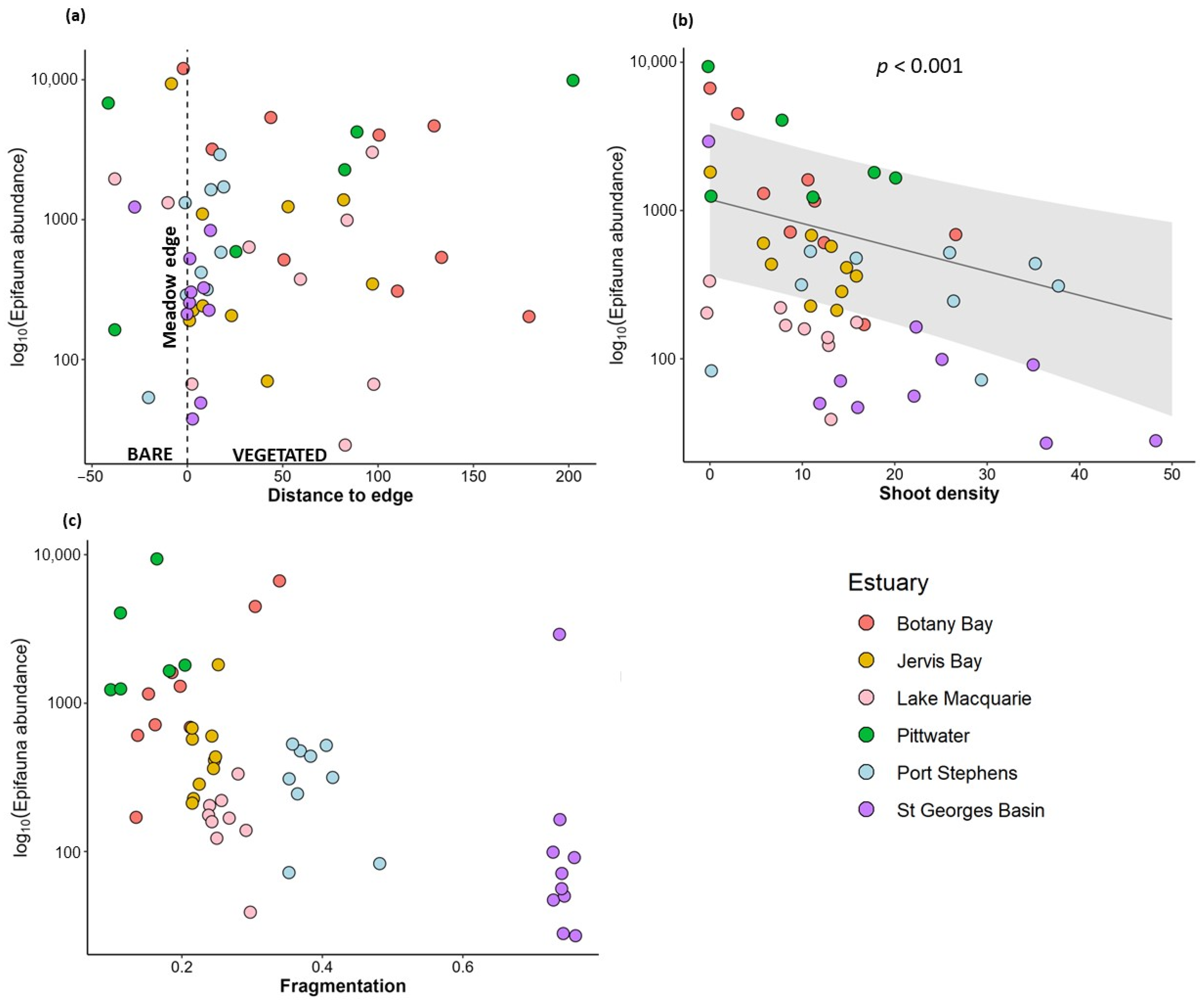
3.1. Variation in Abundance of Epifauna with Habitat Complexity

A total of 55,224 individuals of mobile epifauna were counted across the six meadows, with abundance ranging from 23,272 invertebrates collected at Pittwater and 17,752 at Botany Bay to only 1692 invertebrates collected at Lake Macquarie. Amphipod crustaceans accounted for 82% of all individuals collected, with 10% from the family Caprellidae, followed by polychaete worms (5.4%). Total abundance of epifauna was significantly higher in areas with lower seagrass density (p < 0.001, Figure 3b, Table 1), where seagrass density was the only significant predictor.

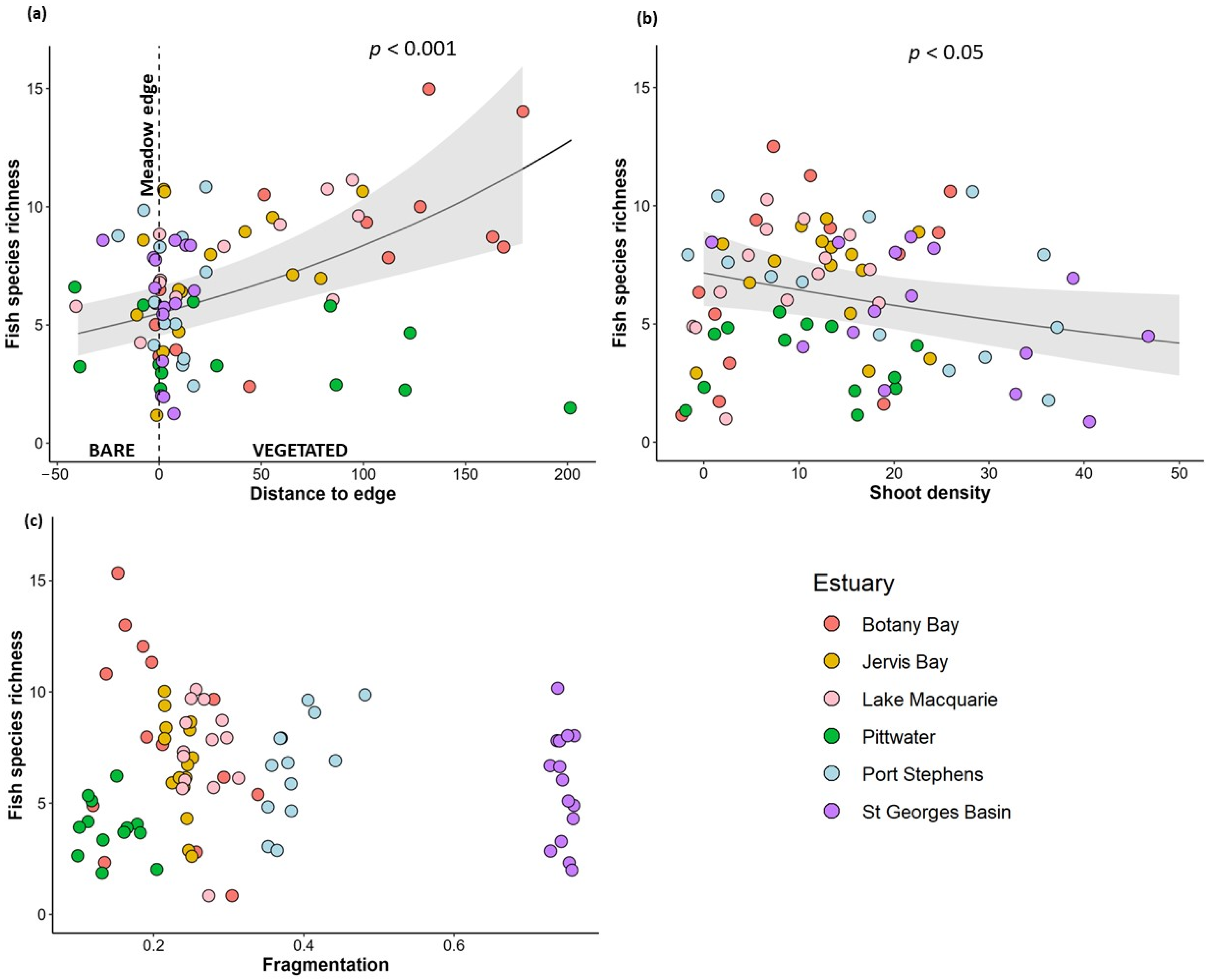
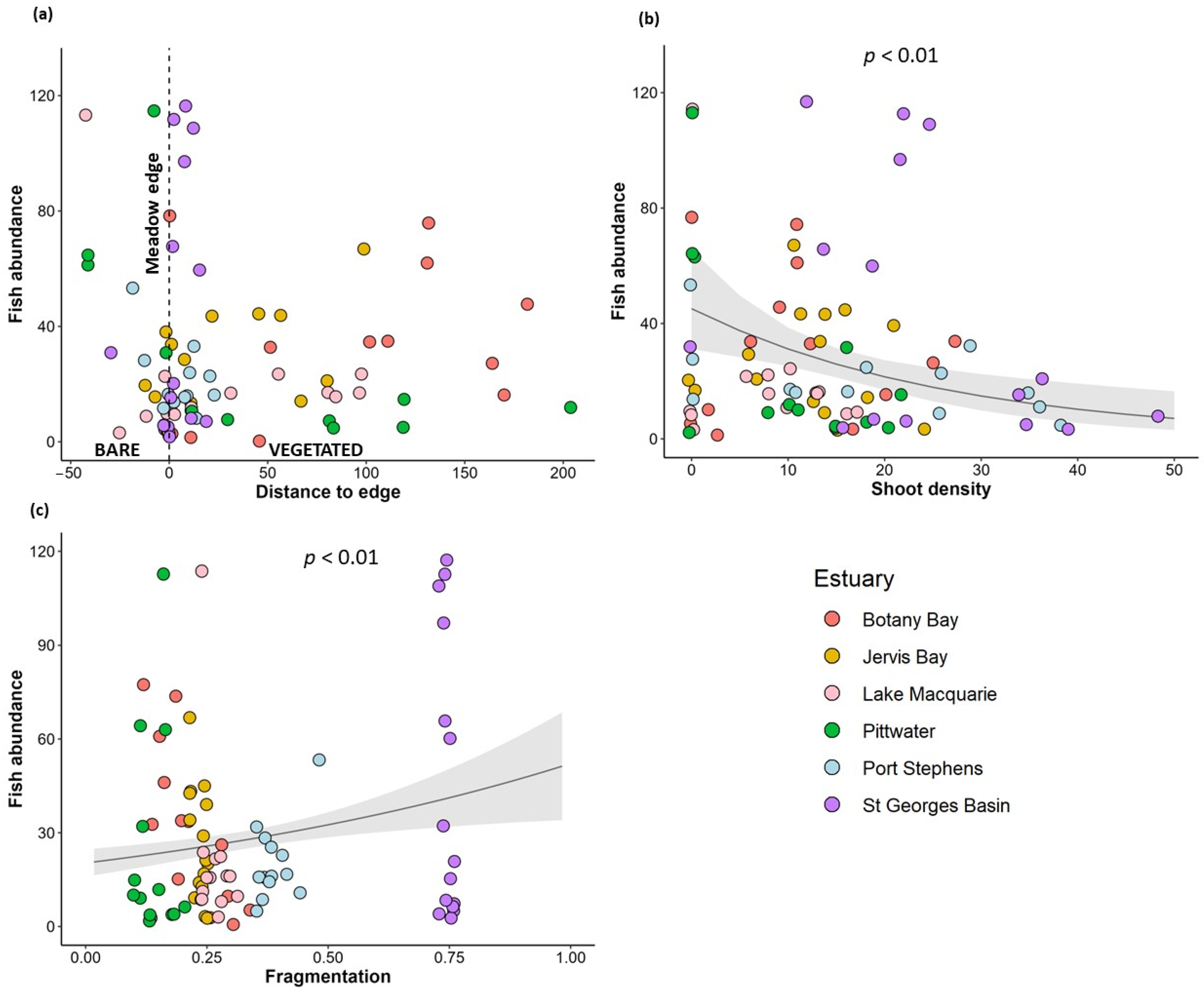
3.2. Variation in Fish Community with Habitat Complexity

A total of 52 species of fish were observed across the six meadows (Table S3), ranging from 31 species in Jervis Bay to 20 species in St Georges Basin and Pittwater. Fish richness declined with increasing seagrass density (p < 0.05, Figure 4b, Table 1) and increasing distance to patch edge (p < 0.001, Figure 4a, Table 1) and was not significantly associated with seagrass fragmentation (Figure 4c, Table 1).
A total of 2385 fish (sum of MaxN) were observed during the study across the six meadows, ranging from 265 in Port Stephens to 663 in St Georges Basin. The total relative abundance of fish decreased with increasing seagrass density (p < 0.01, Figure 5b, Table 1). Total relative abundance of fish also increased with increasing seagrass fragmentation (p < 0.01, Figure 5c, Table 1) but did not vary with distance to edge of a patch (Figure 5a, Table 1).
Most fish species were carnivorous (n = 30), 16 were omnivores, four were planktivores and only two were herbivores (Table S1). Total relative abundance of carnivorous fishes declined with increasing seagrass density (p < 0.001), increased with increasing seagrass fragmentation (p < 0.001) and did not vary with distance to edge. Total relative abundance of herbivores only declined with increased fragmentation (p < 0.05). The relative abundance of the other groups of fish (omnivores and planktivores) was not significantly associated with any of the predictor variables.

3.3. Variation in Erosion with Habitat Complexity

Sediment erosion (ranging from 0 to 16 cm over the entire sampling time) varied with seagrass density (p < 0.01, Table 1), with denser P. australis having the least erosion. No other predictor variables were associated with changes in erosion.

3.4. Variation in Predation Rates with Habitat Complexity

On average, 31% (±10%) of squid pops were eaten after 1 h and 71% were eaten after 24 h (±13%) across the six estuaries. Predation rates had no significant relationship with any of the measured biotic variables (Table 1).

4. Discussion

This study adds to our understanding of the relationships between structural attributes of seagrass meadows and their associated biotic assemblages and functional processes. We tested how a range of habitat complexity measures (at within-patch to seascape scales) influenced functional habitat provisioning for fish and invertebrate communities, along with rates of predation and sediment erosion in six seagrass meadows. Fish were more abundant in areas with high levels of habitat fragmentation and both fish and epifauna were less abundant where seagrass density was greatest. We found lower fish species richness in areas with denser seagrass, but richness was higher in vegetated areas further from patch edges (seagrass density did not correlate with distance to patch edge). Similar to other studies, sediment erosion was reduced in densely vegetated areas [30]. These findings highlight the complexity of the relationship between habitat spatial configuration and functional habitat provision.

4.1. Habitat Use and Predation by Fish

While there were some consistent patterns in habitat use and predation responses to habitat structure across the six estuaries, these patterns did not always match the general patterns in the literature. In contrast to previous studies [29,36,81]; but see [42], we found that fish abundance and richness declined with increases in seagrass density, which represented the smallest scale at which habitat complexity was measured. Accordingly, there was no indication of a threshold level of shoot density that ensured the use of seagrass meadows by fish. However, we acknowledge that the environmental differences among the estuaries may have influenced some of the results (Table S1; [61]). The sampled meadows displayed variable ranges of shoot density (as per [82]): the seagrass in St Georges Basin reached 50 shoots/0.0625 m2 (~800 shoots/m2) while the meadows in all other estuaries had between 10–30 shoots/0.0625 m2 (~160–480 shoots/m2). This is not entirely unexpected, as species assemblages often differ between low and high densities of seagrass [36] and not all fish species respond to seagrass density [83]. The majority of the fish observed were classified as carnivores and they were the only ones influenced by seagrass density (less fish in denser seagrass), suggesting that most fish observed here are not driven by the need of finding refuge but perhaps by presence of other smaller fish as prey. While not addressed within this study, some of the fish sampled here may be residents of the meadow [46], and thus may be more affected by seagrass density than transient species. Detecting fish where vegetation is particularly dense may also require more detailed methods than remote cameras [84,85,86]. This sampling method mostly detected the supra-canopy fishes associated with the meadow whereas methods such as visual census may be more appropriate for sampling within-canopy species [86].
Habitat fragmentation appears to be an inconsistent but important driver of fish species richness and abundance at seascape scales. In this study, fish abundance increased with fragmentation, supporting that seascape-scale spatial arrangement of habitats influenced seagrass fish communities [87]. This relationship was driven by the fish species belonging to the carnivore functional group and may be related to a predatory behaviour that is facilitated in a more fragmented habitat. In contrast, herbivorous fish were less abundant in more fragmented areas. Fragmented seagrass beds may create a more diverse habitat, with seagrass interspersed with bare sediments, attracting fish with different habitat preferences [88]. There was not, however, evidence of a relationship between fish species richness and fragmentation in this study. The greater fish richness observed in vegetated sites toward the middle of the meadow in this study may suggest that many fish we observed may be utilising the seagrass meadows both as a refuge and for foraging [28]. However, there was no evidence that the abundance of any functional groups was significantly influenced by distance to edge. Fish communities can be more abundant and diverse at seagrass edges [89,90] and responses to edges are often species-specific [89,91] or depend on patch size [39]. In contrast, this study did not detect positive edge effects on fish communities. This result may be explained by the variability of responses by the species sampled as some may have a stronger association with interior areas, others with edges or with both habitats [39,92]. Many individuals observed in this study were juveniles (pers. obs.), providing support for the utility of seagrass beds as a preferred nursery area [45,93].
In this study, predation was not influenced by any variables. Predation success and foraging are often greater in more fragmented areas [94,95] or at edges [96], however, presence of top-level predators (not targeted in this study) may alter this relationship [97,98] by inducing a predator avoidance behaviour. Although the squid-pop technique is commonly used worldwide [76], it may be targeting only a limited range of fish species [94]. The high rate of squid pop consumption overnight may be explained by diel migration of some species of fish between vegetated and bare habitat [33]. This can often be the reason of a greater abundance of fish in seagrass beds at night [99,100].

4.2. Use of Seagrass Habitats by Invertebrate Epifauna

We observed greater numbers of invertebrates in less dense seagrass areas. This is in contrast with some previous results, that showed more abundant epifauna in areas with higher P. australis densities due to animals preference for more complex habitat [48]. Predation success may be reduced in dense vegetation [93,101], however, there may be exceptions related to the predatory behaviours, as ambush predators are not be negatively impacted by vegetation [102,103]. Mobile invertebrates are often more abundant in complex habitats with high levels of epiphytes [56], rather than greater macrophyte complexity [70,104]. This may explain, beyond the effect of the large range of shoot density sampled here, the more abundant epifauna found where epiphytic algae grew or drifted on the deployed artificial seagrass (Botany Bay and Pittwater, pers. obs.). Epiphyte abundance and composition could also be driven by the presence of seagrass detritus, with some species using it as food source or as physical habitat [105].
Previous studies have found that proximity to the edge of seagrass meadows strongly influenced epifauna abundance, with different patterns depending on the epifauna group e.g., cumaceans increase at edges, while amphipods decline from seagrass to sand; [106]). We did not find any edge-effect, with this study adding to those that have found variable responses of epifauna to edges, including those with a greater abundance of invertebrates [40,107] or those finding that habitat centres have more abundant invertebrates [108].

4.3. Variation in Erosion with Seagrass Density

Sediment erosion was reduced in denser areas. This supports the critical function of seagrasses at reducing erosion and sediment movement by trapping and stabilising sediments [30,109,110]. Coastal erosion is affecting coasts worldwide and is often combatted through shore nourishment (i.e., deliberate placement of sand to restore a beach) or coastal hard constructions (e.g., groynes and breakwaters; [111]). These solutions are, however, usually temporary and not very cost-efficient at a long term and can further alter local hydrodynamic conditions [109,111]. On the other hand, protecting and restoring vegetated beach foreshore habitats helps stabilise sediments and creates a natural self-sustaining system [112].

4.4. Future Directions

A key consideration after this study is that undertaking a “seascape” approach may provide highly valuable insights to understand faunal assemblages associated with seagrass. The application of techniques developed in landscape ecology can help unravel what drives the communities that inhabit and utilise marine habitats [6,56,59,113]. Understanding how processes and faunal communities respond to different components of a habitat is critical for modern conservation and restoration, as critical foundation species continue to decline globally [114,115]. Therefore, incorporating landscape-scale approach into site selection can improve restoration success [116].
Habitat connectivity is a major driver for the distribution of fauna in marine systems [34,87,117] and, although not directly measured in this study, it needs to be mentioned as the sampled areas displayed some different environmental characteristics (Table S1, Figure 1; [61]). Greater connectivity may reduce the impacts of urbanisation for more resilient species [118]. The types of surrounding habitats, their complexity and their spatial connections can influence marine communities [119,120,121] for example by shaping fish movements. Individual fish can rely on different habitats, move among them with the tides, time of day and during different stages of their life [29]. The presence of different surrounding habitats may enhance fish abundance and species [58] as they tend to prefer habitats with high diversity and high connectivity [87]. A more detailed interrogation including seascape variables such as distance from natural reefs, mangroves and saltmarshes may contribute to explaining some of the patterns.
Differences in environmental variables among sites/estuaries may have influenced some of the outcomes of this study, including the types of species present in the meadows of P. australis. Meadows in Port Stephens and in St Georges Basin were particularly narrow as the depth dropped very quickly into bare sediment, which may explain the high fragmentation and the small range in distance to edge. Port Stephens, Lake Macquarie, Pittwater and Botany Bay are located in catchments with a large human population density relative to Jervis Bay and St Georges Basin, and human activities could influence the estuaries differently. Different fishing pressure among estuaries may have also played a role in the variability among sites, for example commercial fishing is no longer permitted in Lake Macquarie, Botany Bay or St Georges Basin. Although Port Stephens and Jervis Bay estuaries are within marine parks, the specific sites sampled in these estuaries were not in fishing exclusion (sanctuary) zones. The morphological characterises of the estuaries and position of each site relative to the mouth of the estuary also differed, which may affect water exchange and perhaps fish or invertebrate assemblages. However, estuaries were similar enough to enable P. australis to grow (such characteristics are found in only 17 of 121 seagrass estuaries in NSW [50]). Future studies could benefit from sampling multiple meadows (with different levels of fragmentation) in each estuary.
This study advanced understanding about what structural characteristics of P. australis meadows drive biotic assemblages and can inform strategies to manage endangered seagrass habitats by informing decisions for future restorations, e.g., identifying specific meadow structural traits that may be targeted during conservation or restoration projects. For example, to reduce coastal erosion, the restoration target would include higher seagrass densities, supporting the thesis that seagrasses are critical at stabilising coastlines [109], while to ensure high species richness of fish, it may be preferable to protect vegetated areas further from the edge. On the other hand, if the target is to enhance biodiversity and improve habitat provision, these results showed no evidence of a seagrass density threshold, meaning that benefits of restoration can be achieved without necessarily restoring meadows to the highest natural densities observed (e.g., fish were supported across a wide range of shoot densities). In conclusion, despite observing high variation in relationships with habitat provisioning, there is clear value in considering habitat spatial patterns at multiple scales in seagrass systems.

Supplementary Materials

The following supporting information can be downloaded at: https://www.mdpi.com/article/10.3390/d15020125/s1, Table S1: Environmental characteristics and aspects of the ecology of the six estuaries sampled in this study, based on [61,122,123]. NA—no commercial fishing in these estuaries. Table S2: List of the sampling sites and variables obtained using Generalised Random Tessellation Structures (GRTS). Site ‘ps7′ was not included in the analyses because too deep and not representative of a seagrass habitat. Table S3: list of fish species observed in the videos, including species functional traits (feeding information) [29,46,61,122,123,124,125,126]; Figure S1: example of (a) an artificial Posidonia unit in a seagrass patch and (b) in a bare area and (c) of a supra-canopy GoPro set up; Figure S2: correlation plots among variables: distance to patch edge, seagrass shoot density, area and level of fragmentation at 50 m, 250 m and 500 m of radius.

Author Contributions

Conceptualization, G.F., A.G.B.P., A.V., T.M.G. and K.J.G.; Methodology, G.F., A.G.B.P., A.V., T.M.G. and K.J.G.; Formal Analysis, G.F., A.G.B.P., K.J.G.; Investigation, G.F., K.J.G.; Writing—Original Draft Preparation, G.F.; Writing—Review and Editing, G.F., A.G.B.P., A.V., T.M.G. and K.J.G.; Visualization, G.F. and A.G.B.P.; Funding Acquisition, G.F., A.G.B.P., A.V. and T.M.G. All authors have read and agreed to the published version of the manuscript.

Funding

This research was funded by Sea World Research and Rescue Foundation, grant number SWR/8/2019.

Institutional Review Board Statement

Work was carried out under NSW DPI Fisheries Section 37 permit (P13/0007-2.0), a NSW Marine Parks Permit and Animal Ethics ACEC 19/9B.

Informed Consent Statement

Not applicable.

Data Availability Statement

The data presented in this study are available on request from the corresponding author.

Acknowledgments

For assistance with field work we thank Derrick Cruz, Madelaine Langley, Javier Jimenez, Paula Sgarlatta, Chris Roberts, Sam Nolan, Olavo Bueno and Barbara Sanna Godoi. We also thank UNSW volunteers for their help in sorting epifauna in the lab: Alexandra Laitly, Chloe Brant, Morna McGuire, Hadi Esmaeil, Kathy Liu, Itasca Motter, Alex Ingall, Kiki Liang, Daphne Willemsen, Rosie Dowsett, Tom Chaffey, Melissa Abdallah, Jessica Nguyen, Cameron Suen. Daniel Swadling and Emma Jackson provided useful feedback on the manuscript.

Conflicts of Interest

The authors declare no conflict of interest.

References

  1. Kovalenko, K.E.; Thomaz, S.M.; Warfe, D.M. Habitat complexity: Approaches and future directions. Hydrobiologia 2012, 685, 1–17. [Google Scholar] [CrossRef]
  2. MacArthur, R.H.; MacArthur, J.W. On Bird Species Diversity. Ecology 1961, 42, 594–598. [Google Scholar] [CrossRef]
  3. Denno, R.F.; Finke, D.L.; Langellotto, G.A. Direct and indirect effects of vegetation structure and habitat complexity on predator-prey and predator-predator interactions. In Ecology of Predator-Prey Interactions; Oxford University: Oxford, UK, 2005; pp. 211–239. [Google Scholar]
  4. Warfe, D.M.; Barmuta, L. Habitat structural complexity mediates the foraging success of multiple predator species. Oecologia 2004, 141, 171–178. [Google Scholar] [CrossRef]
  5. Farina, S.; Arthur, R.; Pagès, J.; Prado, P.; Romero, J.; Verges, A.; Hyndes, G.; Heck, K.L.; Glenos, S.; Alcoverro, T. Differences in predator composition alter the direction of structure-mediated predation risk in macrophyte communities. Oikos 2014, 123, 1311–1322. [Google Scholar] [CrossRef] [Green Version]
  6. Boström, C.; Pittman, S.; Simenstad, C.; Kneib, R. Seascape ecology of coastal biogenic habitats: Advances, gaps, and challenges. Mar. Ecol. Prog. Ser. 2011, 427, 191–217. [Google Scholar] [CrossRef] [Green Version]
  7. Haddad, N.M.; Brudvig, L.A.; Clobert, J.; Davies, K.F.; Gonzalez, A.; Holt, R.D.; Lovejoy, T.E.; Sexton, J.O.; Austin, M.P.; Collins, C.D.; et al. Habitat fragmentation and its lasting impact on Earth’s ecosystems. Sci. Adv. 2015, 1, e1500052. [Google Scholar] [CrossRef] [PubMed] [Green Version]
  8. Wilson, M.C.; Chen, X.-Y.; Corlett, R.T.; Didham, R.K.; Ding, P.; Holt, R.D.; Holyoak, M.; Hu, G.; Hughes, A.C.; Jiang, L.; et al. Habitat fragmentation and biodiversity conservation: Key findings and future challenges. Landsc. Ecol. 2016, 33, 341–352. [Google Scholar]
  9. Bustamante, M.M.C.; Roitman, I.; Aide, T.M.; Alencar, A.; Anderson, L.O.; Aragão, L.; Asner, G.P.; Barlow, J.; Berenguer, E.; Chambers, J.; et al. Toward an integrated monitoring framework to assess the effects of tropical forest degradation and recovery on carbon stocks and biodiversity. Glob. Chang. Biol. 2016, 22, 92–109. [Google Scholar] [CrossRef] [PubMed] [Green Version]
  10. Fahrig, L. Ecological Responses to Habitat Fragmentation Per Se. Annu. Rev. Ecol. Evol. Syst. 2017, 48, 1–23. [Google Scholar] [CrossRef]
  11. Halpern, B.S.; Walbridge, S.; Selkoe, K.A.; Kappel, C.V.; Micheli, F.; D’Agrosa, C.; Bruno, J.F.; Casey, K.S.; Ebert, C.; Fox, H.E.; et al. A global map of human impact on marine ecosystems. Science 2008, 319, 948–952. [Google Scholar] [CrossRef] [Green Version]
  12. Berger-Tal, O.; Saltz, D. Invisible barriers: Anthropogenic impacts on inter- and intra-specific interactions as drivers of landscape-independent fragmentation. Philos. Trans. R. Soc. B Biol. Sci. 2019, 374, 20180049. [Google Scholar] [CrossRef]
  13. Delarue, E.M.P.; Kerr, S.E.; Rymer, T.L. Habitat complexity, environmental change and personality: A tropical perspective. Behav. Process. 2015, 120, 101–110. [Google Scholar] [CrossRef]
  14. Hooper, D.U.; Adair, E.C.; Cardinale, B.J.; Byrnes, J.E.K.; Hungate, B.A.; Matulich, K.L.; Gonzalez, A.; Duffy, J.E.; Gamfeldt, L.; O’Connor, M.I. A global synthesis reveals biodiversity loss as a major driver of ecosystem change. Nature 2012, 486, 105–108. [Google Scholar] [CrossRef]
  15. Hooper, D.U.; Chapin, F.S., III; Ewel, J.J.; Hector, A.; Inchausti, P.; Lavorel, S.; Lawton, J.H.; Lodge, D.M.; Loreau, M.; Naeem, S.; et al. Effects of biodiversity on ecosystem functioning: A consensus of current knowledge. Ecol. Monogr. 2005, 75, 3–35. [Google Scholar] [CrossRef]
  16. Thompson, I.; Mackey, B.; McNulty, S.; Mosseler, A. Forest Resilience, Biodiversity, and Climate Change; Technical Series no. 43; Secretariat of the Convention on Biological Diversity: Montreal, QC, Canada, 2009; pp. 1–67. [Google Scholar]
  17. Duffy, J.E.; Godwin, C.M.; Cardinale, B.J. Biodiversity effects in the wild are common and as strong as key drivers of productivity. Nature 2017, 549, 261–264. [Google Scholar] [CrossRef]
  18. Cardinale, B.J.; Duffy, J.E.; Gonzalez, A.; Hooper, D.U.; Perrings, C.; Venail, P.; Narwani, A.; Mace, G.M.; Tilman, D.; Wardle, D.A.; et al. Biodiversity loss and its impact on humanity. Nature 2012, 486, 59–67. [Google Scholar] [CrossRef] [Green Version]
  19. Sintayehu, D.W. Impact of climate change on biodiversity and associated key ecosystem services in Africa: A systematic review. Ecosyst. Health Sustain. 2018, 4, 225–239. [Google Scholar] [CrossRef] [Green Version]
  20. Ellison, A.M.; Bank, M.S.; Clinton, B.D.; Colburn, E.A.; Elliott, K.; Ford, C.R.; Foster, D.R.; Kloeppel, B.D.; Knoepp, J.D.; Lovett, G.M.; et al. Loss of foundation species: Consequences for the structure and dynamics of forested ecosystems. Front. Ecol. Environ. 2005, 3, 479–486. [Google Scholar] [CrossRef]
  21. Toenies, M.J.; Miller, D.A.W.; Marshall, M.R.; Stauffer, G.E. Shifts in vegetation and avian community structure following the decline of a foundational forest species, the eastern hemlock. Ornithol. Appl. 2018, 120, 489–506. [Google Scholar] [CrossRef]
  22. Wernberg, T.; Krumhansl, K.; Filbee-Dexter, K.; Pedersen, M.F. Status and trends for the world’s kelp forests. In World Seas: An Environmental Evaluation; Elsevier: Amsterdam, The Netherlands, 2019; pp. 57–78. [Google Scholar]
  23. Burgos, E.; Montefalcone, M.; Ferrari, M.; Paoli, C.; Vassallo, P.; Morri, C.; Bianchi, C.N. Ecosystem functions and economic wealth: Trajectories of change in seagrass meadows. J. Clean. Prod. 2017, 168, 1108–1119. [Google Scholar] [CrossRef]
  24. Dunic, J.C.; Brown, C.J.; Connolly, R.M.; Turschwell, M.P.; Côté, I.M. Long-term declines and recovery of meadow area across the world’s seagrass bioregions. Glob. Change Biol. 2021, 27, 4096–4109. [Google Scholar] [CrossRef] [PubMed]
  25. Duffy, J. Biodiversity and the functioning of seagrass ecosystems. Mar. Ecol. Prog. Ser. 2006, 311, 233–250. [Google Scholar] [CrossRef] [Green Version]
  26. Lavery, P.S.; Mateo, M.; Serrano, O.; Rozaimi, M. Variability in the Carbon Storage of Seagrass Habitats and Its Implications for Global Estimates of Blue Carbon Ecosystem Service. PLoS ONE 2013, 8, e73748. [Google Scholar] [CrossRef] [PubMed] [Green Version]
  27. Ricart, A.M.; York, P.H.; Bryant, C.V.; Rasheed, M.A.; Ierodiaconou, D.; Macreadie, P.I. High variability of Blue Carbon storage in seagrass meadows at the estuary scale. Sci. Rep. 2020, 10, 5865. [Google Scholar] [CrossRef] [PubMed] [Green Version]
  28. Jackson, E.L.; Rowden, A.A.; Attrill, M.J.; Bossey, S.J.; Jones, M.B. The importance of seagrass beds as a habitat for fishery species. Oceanogr. Mar. Biol. 2001, 39, 269–304. [Google Scholar]
  29. Gillanders, B.M. Seagrasses, fish, and fisheries. In Seagrasses: Biology, Ecology and Conservation; Springer: Berlin/Heidelberg, Germany, 2007; pp. 503–505. [Google Scholar]
  30. Potouroglou, M.; Bull, J.C.; Krauss, K.W.; Kennedy, H.A.; Fusi, M.; Daffonchio, D.; Mangora, M.M.; Githaiga, M.N.; Diele, K.; Huxham, M. Measuring the role of seagrasses in regulating sediment surface elevation. Sci. Rep. 2017, 7, 11917. [Google Scholar] [CrossRef] [Green Version]
  31. Gray, C.; McElligott, D.; Chick, R.; Chick, R. Intra- and inter-estuary differences in assemblages of fishes associated with shallow seagrass and bare sand. Mar. Freshw. Res. 1996, 47, 723–735. [Google Scholar] [CrossRef]
  32. Ferrell, D.; Bell, J. Differences among assemblages of fish associated with Zostera capricorni and bare sand over a large spatial scale. Mar. Ecol. Prog. Ser. 1991, 72, 15–24. [Google Scholar] [CrossRef]
  33. Jackson, E.L.; Rowden, A.A.; Attrill, M.J.; Bossy, S.F.; Jones, M.B. Comparison of fish and mobile macroinvertebrates associated with seagrass and adjacent sand at St. Catherine Bay, Jersey (English Channel): Emphasis on commercial species. Bull. Mar. Sci. 2002, 71, 1333–1341. [Google Scholar]
  34. Boström, C.; Jackson, E.L.; Simenstad, C.A. Seagrass landscapes and their effects on associated fauna: A review. Estuar. Coast. Shelf Sci. 2006, 68, 383–403. [Google Scholar] [CrossRef]
  35. Curtis, J.; Vincent, A. Distribution of sympatric seahorse species along a gradient of habitat complexity in a seagrass-dominated community. Mar. Ecol. Prog. Ser. 2005, 291, 81–91. [Google Scholar] [CrossRef]
  36. McCloskey, R.M.; Unsworth, R.K. Decreasing seagrass density negatively influences associated fauna. PeerJ 2015, 3, e1053. [Google Scholar] [CrossRef] [PubMed] [Green Version]
  37. Staveley, T.A.B.; Perry, D.; Lindborg, R.; Gullström, M. Seascape structure and complexity influence temperate seagrass fish assemblage composition. Ecography 2016, 40, 936–946. [Google Scholar] [CrossRef]
  38. Bologna, P.A.X.; Heck, K.L. Impact of habitat edges on density and secondary production of seagrass-associated fauna. Estuaries 2002, 25, 1033–1044. [Google Scholar] [CrossRef]
  39. Smith, T.; Hindell, J.S.; Jenkins, G.P.; Connolly, R.M. Seagrass patch size affects fish responses to edges. J. Anim. Ecol. 2009, 79, 275–281. [Google Scholar] [CrossRef] [Green Version]
  40. Tanner, J.E. Edge effects on fauna in fragmented seagrass meadows. Austral Ecol. 2005, 30, 210–218. [Google Scholar] [CrossRef]
  41. Gilby, B.; Olds, A.; Connolly, R.; Maxwell, P.; Henderson, C.; Schlacher, T. Seagrass meadows shape fish assemblages across estuarine seascapes. Mar. Ecol. Prog. Ser. 2018, 588, 179–189. [Google Scholar] [CrossRef] [Green Version]
  42. Ricart, A.M. Insights into Seascape Ecology: Landscape Patterns as Drivers in Coastal Marine Ecosystems. Doctoral Dissertation, Universitat de Barcelona, Barcelona, Spain, 2016. [Google Scholar]
  43. González-Ortiz, V.; Egea, L.G.; Ramos, R.J.; Moreno-Marín, F.; Perez-Llorens, J.L.; Bouma, T.J.; Brun, F.G. Interactions between Seagrass Complexity, Hydrodynamic Flow and Biomixing Alter Food Availability for Associated Filter-Feeding Organisms. PLoS ONE 2014, 9, e104949. [Google Scholar] [CrossRef] [Green Version]
  44. Folkard, A.M. Hydrodynamics of model Posidonia oceanica patches in shallow water. Limnol. Oceanogr. 2005, 50, 1592–1600. [Google Scholar] [CrossRef]
  45. Middleton, M.; Bell, J.; Burchmore, J.; Pollard, D.; Pease, B. Structural differences in the fish communities of Zostera capricorni and Posidonia australis seagrass meadows in Botany Bay, New South Wales. Aquat. Bot. 1984, 18, 89–109. [Google Scholar] [CrossRef]
  46. Burchmore, J.; Pollard, D.; Bell, J. Community structure and trophic relationships of the fish fauna of an estuarine Posidonia Australis seagrass habitat in port hacking, new South Wales. Aquat. Bot. 1984, 18, 71–87. [Google Scholar] [CrossRef]
  47. Bell, J.D.; Westoby, M. Variation in seagrass height and density over a wide spatial scale: Effects on common fish and decapods. J. Exp. Mar. Biol. Ecol. 1986, 104, 275–295. [Google Scholar] [CrossRef]
  48. Bell, J.D.; Westoby, M. Abundance of macrofauna in dense seagrass is due to habitat preference, not predation. Oecologia 1986, 68, 205–209. [Google Scholar] [CrossRef] [PubMed]
  49. Evans, S.M.; Griffin, K.J.; Blick, R.A.J.; Poore, A.; Vergés, A. Seagrass on the brink: Decline of threatened seagrass Posidonia australis continues following protection. PLoS ONE 2018, 13, e0190370. [Google Scholar] [CrossRef] [PubMed]
  50. West, G.J.; Glasby, T.M. Interpreting Long-Term Patterns of Seagrasses Abundance: How Seagrass Variability Is Dependent on Genus and Estuary Type. Estuaries Coasts 2022, 45, 1393–1408. [Google Scholar] [CrossRef]
  51. Glasby, T.M.; West, G. Dragging the chain: Quantifying continued losses of seagrasses from boat moorings. Aquat. Conserv. Mar. Freshw. Ecosyst. 2018, 28, 383–394. [Google Scholar] [CrossRef]
  52. EPBC Act. Environment Protection and Biodiversity Conservation Act 1999 (EPBC Act) (s266B). Approved Conservation Advice (Including Listing Advice) for Posidonia Australis Seagrass Meadows of the Manning-Hawkesbury Ecoregion Ecological Community; Office of Legislative Drafting and Publishing: Canberra, Australia, 2015. [Google Scholar]
  53. Meehan, A.J.; West, R.J. Recovery times for a damaged Posidonia australis bed in south eastern Australia. Aquat. Bot. 2000, 67, 161–167. [Google Scholar] [CrossRef]
  54. Ferretto, G.; Glasby, T.M.; Poore, A.G.; Callaghan, C.T.; Housefield, G.P.; Langley, M.; Sinclair, E.A.; Statton, J.; Kendrick, G.A.; Vergés, A. Naturally-detached fragments of the endangered seagrass Posidonia australis collected by citizen scientists can be used to successfully restore fragmented meadows. Biol. Conserv. 2021, 262, 109308. [Google Scholar] [CrossRef]
  55. Waltham, N.J.; Elliott, M.; Lee, S.Y.; Lovelock, C.; Duarte, C.M.; Buelow, C.; Simenstad, C.; Nagelkerken, I.; Claassens, L.; Wen, C.K.-C.; et al. UN Decade on Ecosystem Restoration 2021–2030—What chance for success in restoring coastal ecosystems? Front. Mar. Sci. 2020, 7, 71. [Google Scholar] [CrossRef] [Green Version]
  56. Jackson, E.L.; Attrill, M.J.; Jones, M.B. Habitat characteristics and spatial arrangement affecting the diversity of fish and decapod assemblages of seagrass (Zostera marina) beds around the coast of Jersey (English Channel). Estuar. Coast. Shelf Sci. 2006, 68, 421–432. [Google Scholar] [CrossRef]
  57. Boström, C.; Bonsdorff, E. Zoobenthic community establishment and habitat complexity the importance of seagrass shoot-density, morphology and physical disturbance for faunal recruitment. Mar. Ecol. Prog. Ser. 2000, 205, 123–138. [Google Scholar] [CrossRef] [Green Version]
  58. Swadling, D.S.; Knott, N.A.; Rees, M.J.; Davis, A.R. Temperate zone coastal seascapes: Seascape patterning and adjacent seagrass habitat shape the distribution of rocky reef fish assemblages. Landsc. Ecol. 2019, 34, 2337–2352. [Google Scholar] [CrossRef]
  59. Pittman, S.J. Seascape Ecology; John Wiley & Sons: Hoboken, NJ, USA, 2018. [Google Scholar]
  60. Pittman, S.; Yates, K.; Bouchet, P.; Alvarez-Berastegui, D.; Andréfouët, S.; Bell, S.; Berkström, C.; Boström, C.; Brown, C.; Connolly, R.; et al. Seascape ecology: Identifying research priorities for an emerging ocean sustainability science. Mar. Ecol. Prog. Ser. 2021, 663, 1–29. [Google Scholar] [CrossRef]
  61. Roy, P.; Williams, R.; Jones, A.; Yassini, I.; Gibbs, P.; Coates, B.; West, R.; Scanes, P.; Hudson, J.; Nichol, S. Structure and Function of South-east Australian Estuaries. Estuar. Coast. Shelf Sci. 2001, 53, 351–384. [Google Scholar] [CrossRef]
  62. NSW Department of Primary Industries. Fisheries NSW Spatial Data Portal. Available online: https://webmap.industry.nsw.gov.au/Html5Viewer/index.html?viewer=Fisheries_Data_Portal (accessed on 11 February 2019).
  63. Stevens, D.L., Jr.; Olsen, A.R. Spatially balanced sampling of natural resources. J. Am. Stat. Assoc. 2004, 99, 262–278. [Google Scholar] [CrossRef]
  64. Rees, M.; Knott, N.A.; Hing, M.L.; Hammond, M.; Williams, J.; Neilson, J.; Swadling, D.S.; Jordan, A. Habitat and humans predict the distribution of juvenile and adult snapper (Sparidae: Chrysophrys auratus) along Australia’s most populated coastline. Estuar. Coast. Shelf Sci. 2021, 257, 107397. [Google Scholar] [CrossRef]
  65. Sleeman, J.C.; Kendrick, G.; Boggs, G.; Hegge, B. Measuring fragmentation of seagrass landscapes: Which indices are most appropriate for detecting change? Mar. Freshw. Res. 2005, 56, 851–864. [Google Scholar] [CrossRef]
  66. Santos, R.O.; Lirman, D.; Pittman, S.J. Long-term spatial dynamics in vegetated seascapes: Fragmentation and habitat loss in a human-impacted subtropical lagoon. Mar. Ecol. 2015, 37, 200–214. [Google Scholar] [CrossRef]
  67. Bivand, R.; Keitt, T.; Rowlingson, B.; Pebesma, E.; Sumner, M.; Hijmans, R.; Rouault, E.l. Package ‘Rgdal’. Bindings for the Geospatial Data Abstraction Library 2015. Available online: https://CRAN.R-project.org/package=rgdal (accessed on 11 February 2019).
  68. Hijmans, R.J.; van Etten, J.; Sumner, M.; Cheng, J.; Baston, D.; Bevan, A.; Bivand, R.; Busetto, L.; Canty, M.; Fasoli, B.; et al. Package ‘raster’: Geographic Data Analysis and Modeling. 2015. Available online: https://CRAN.R-project.org/package=raster (accessed on 11 February 2019).
  69. Hijmans, R.J.; Karney, C.; Williams, E.; Vennes, C.; Hijmans, R.J. Package ‘geosphere’: Spherical Trigonometry 2017. Available online: https://CRAN.R-project.org/package=geosphere (accessed on 11 February 2019).
  70. Martin-Smith, K.M. Abundance of mobile epifauna: The role of habitat complexity and predation by fishes. J. Exp. Mar. Biol. Ecol. 1993, 174, 243–260. [Google Scholar] [CrossRef]
  71. Cappo, M.; Harvey, E.; Malcolm, H.; Speare, P. Potential of Video Techniques to Monitor Diversity, Abundance and Size of Fish in Studies of Marine Protected Areas; Aquatic Protected Areas-what works best and how do we know; University of Queensland: Brisbane, Australia, 2003; pp. 455–464. [Google Scholar]
  72. Willis, T.J.; Millar, R.B.; Babcock, R.C. Detection of spatial variability in relative density of fishes: Comparison of visual census, angling, and baited underwater video. Mar. Ecol. Prog. Serles 2000, 198, 249–260. [Google Scholar] [CrossRef]
  73. Froese, R.; Pauly, D. FishBase 2000: Concepts, Design and Data Sources; ICLARM: Los Baños, Laguna, Philippines, 2000; 344p. [Google Scholar]
  74. Bray, D.J.; Gomon, M.F.; Fishes of Australia. Museums Victoria and OzFishNet. Available online: https://fishesofaustralia.net.au/ (accessed on 28 April 2022).
  75. McGrouther, M. Australian Museum Website. Available online: https://australian.museum/learn/animals/fishes/ (accessed on 28 April 2022).
  76. Duffy, J.E.; Ziegler, S.; Campbell, J.E.; Bippus, P.M.; Lefcheck, J. Squidpops: A Simple Tool to Crowdsource a Global Map of Marine Predation Intensity. PLoS ONE 2015, 10, e0142994. [Google Scholar] [CrossRef] [PubMed]
  77. Vila-Concejo, A.; Harris, D.L.; Power, H.E.; Shannon, A.M.; Webster, J.M. Sediment transport and mixing depth on a coral reef sand apron. Geomorphology 2014, 222, 143–150. [Google Scholar] [CrossRef]
  78. Brooks, M.E.; Kristensen, K.; van Benthem, K.J.; Magnusson, A.; Berg, C.W.; Nielsen, A.; Skaug, H.J.; Maechler, M.; Bolker, B.M. GlmmTMB Balances Speed and Flexibility Among Packages for Zero-inflated Generalized Linear Mixed Modeling. The R Journal 2017, 9, 378–400. [Google Scholar] [CrossRef]
  79. Wickham, H.; Averick, M.; Bryan, J.; Chang, W.; D’Agostino McGowan, L.; François, R.; Grolemund, G.; Hayes, A.; Henry, L.; Hester, J.; et al. Welcome to the Tidyverse. J. Open Source Softw. 2019, 4, 1686. [Google Scholar] [CrossRef] [Green Version]
  80. Wickham, H. Ggplot2: Elegant Graphics for Data Analysis; Springer: Berlin/Heidelberg, Germany, 2016. [Google Scholar]
  81. Heck, K.L., Jr.; Orth, R.J. Seagrass habitats: The roles of habitat complexity, competition and predation in structuring associated fish and motile macroinvertebrate assemblages. In Estuarine Perspectives; Elsevier: Amsterdam, The Netherlands, 1980; pp. 449–464. [Google Scholar]
  82. Worthington, D.; Ferrell, D.J.; McNeill, S.E.; Bell, J.D. Effects of the shoot density of seagrass on fish and decapods: Are correlation evident over larger spatial scales? Mar. Biol. 1992, 112, 139–146. [Google Scholar] [CrossRef]
  83. Bell, J.D.; Westoby, M. Importance of local changes in leaf height and density to fish and decapods associated with seagrasses. J. Exp. Mar. Biol. Ecol. 1986, 104, 249–274. [Google Scholar] [CrossRef]
  84. Kiggins, R.S.; Knott, N.A.; Davis, A.R. Miniature baited remote underwater video (mini-BRUV) reveals the response of cryptic fishes to seagrass cover. J. Appl. Phycol. 2018, 101, 1717–1722. [Google Scholar] [CrossRef] [Green Version]
  85. Swadling, D.S.; Knott, N.A.; Rees, M.J.; Pederson, H.; Adams, K.R.; Taylor, M.D.; Davis, A.R. Seagrass canopies and the performance of acoustic telemetry: Implications for the interpretation of fish movements. Anim. Biotelem. 2020, 8, 8. [Google Scholar] [CrossRef] [Green Version]
  86. French, B.; Wilson, S.; Holmes, T.; Kendrick, A.; Rule, M.; Ryan, N. Comparing five methods for quantifying abundance and diversity of fish assemblages in seagrass habitat. Ecol. Indic. 2021, 124, 107415. [Google Scholar] [CrossRef]
  87. Henderson, C.J.; Gilby, B.L.; Lee, S.Y.; Stevens, T. Contrasting effects of habitat complexity and connectivity on biodiversity in seagrass meadows. Mar. Biol. 2017, 164, 117. [Google Scholar] [CrossRef]
  88. Horinouchi, M.; Tongnunui, P.; Nanjyo, K.; Nakamura, Y.; Sano, M.; Ogawa, H. Differences in fish assemblage structures between fragmented and continuous seagrass beds in Trang, southern Thailand. Fish. Sci. 2009, 75, 1409–1416. [Google Scholar] [CrossRef]
  89. Smith, T.; Hindell, J.S.; Jenkins, G.P.; Connolly, R.M. Edge effects on fish associated with seagrass and sand patches. Mar. Ecol. Prog. Ser. 2008, 359, 203–213. [Google Scholar] [CrossRef] [Green Version]
  90. Macreadie, P.I.; Hindell, J.S.; Jenkins, G.P.; Connolly, R.M.; Keough, M.J. Fish Responses to Experimental Fragmentation of Seagrass Habitat. Conserv. Biol. 2009, 23, 644–652. [Google Scholar] [CrossRef] [PubMed]
  91. Macreadie, P.I.; Hindell, J.S.; Keough, M.J.; Jenkins, G.P.; Connolly, R.M. Resource distribution influences positive edge effects in a seagrass fish. Ecology 2010, 91, 2013–2021. [Google Scholar] [PubMed]
  92. Bender, D.J.; Contreras, T.A.; Fahrig, L. Habitat loss and population decline: A meta-analysis of the patch size effect. Ecology 1998, 79, 517–533. [Google Scholar] [CrossRef]
  93. Heck, K., Jr.; Hays, G.; Orth, R.J. Critical evaluation of the nursery role hypothesis for seagrass meadows. Mar. Ecol. Prog. Ser. 2003, 253, 123–136. [Google Scholar] [CrossRef] [Green Version]
  94. Yarnall, A.H.; Fodrie, F.J. Predation patterns across states of landscape fragmentation can shift with seasonal transitions. Oecologia 2020, 193, 403–413. [Google Scholar] [CrossRef]
  95. Irlandi, E.A. Large- and small-scale effects of habitat structure on rates of predation: How percent coverage of seagrass affects rates of predation and siphon nipping on an infaunal bivalve. Oecologia 1994, 98, 176–183. [Google Scholar] [CrossRef]
  96. Smith, T.M.; Hindell, J.S.; Jenkins, G.P.; Connolly, R.; Keough, M.J. Edge effects in patchy seagrass landscapes: The role of predation in determining fish distribution. J. Exp. Mar. Biol. Ecol. 2011, 399, 8–16. [Google Scholar] [CrossRef]
  97. Hovel, K.A.; Regan, H.M. Using an individual-based model to examine the roles of habitat fragmentation and behavior on predator–prey relationships in seagrass landscapes. Landsc. Ecol. 2007, 23, 75–89. [Google Scholar] [CrossRef]
  98. Lester, E.K.; Langlois, T.J.; Simpson, S.D.; McCormick, M.I.; Meekan, M.G. Reef-wide evidence that the presence of sharks modifies behaviors of teleost mesopredators. Ecosphere 2021, 12, e03301. [Google Scholar] [CrossRef]
  99. Lubbers, L.; Boynton, W.; Kemp, W. Variations in structure of estuarine fish communities in relation to abundance of submersed vascular plants. Mar. Ecol. Prog. Ser. 1990, 65, 1–14. [Google Scholar] [CrossRef]
  100. Olney, J.; Boehlert, G. Nearshore ichthyoplankton associated with seagrass beds in the lower Chesapeake Bay. Mar. Ecol. Prog. Ser. 1988, 45, 33–43. [Google Scholar] [CrossRef]
  101. Orth, R.J.; Heck, K.L.; van Montfrans, J. Faunal Communities in Seagrass Beds: A Review of the Influence of Plant Structure and Prey Characteristics on Predator: Prey Relationships. Estuaries 1984, 7, 339–350. [Google Scholar] [CrossRef]
  102. James, P.L.; Heck, K.L. The effects of habitat complexity and light intensity on ambush predation within a simulated seagrass habitat. J. Exp. Mar. Biol. Ecol. 1994, 176, 187–200. [Google Scholar] [CrossRef]
  103. Heck, K.L., Jr.; Orth, R.J. Predation in Seagrass Beds. In Seagrasses: Biology, Ecology and Conservation; Springer: Berlin/Heidelberg, Germany, 2006; pp. 537–550. [Google Scholar]
  104. Edgar, G.J. Artificial algae as habitats for mobile epifauna: Factors affecting colonization in a Japanese Sargassum bed. Hydrobiologia 1991, 226, 111–118. [Google Scholar] [CrossRef]
  105. Costa, V.; Chemello, R.; Iaciofano, D.; Brutto, S.L.; Rossi, F. Small-scale patches of detritus as habitat for invertebrates within a Zostera noltei meadow. Mar. Environ. Res. 2021, 171, 105474. [Google Scholar] [CrossRef]
  106. Macreadie, P.I.; Connolly, R.M.; Jenkins, G.P.; Hindell, J.S.; Keough, M.J. Edge patterns in aquatic invertebrates explained by predictive models. Mar. Freshw. Res. 2010, 61, 214–218. [Google Scholar] [CrossRef] [Green Version]
  107. Lanham, B.S.; Poore, A.G.; Gribben, P.E. Fine-scale responses of mobile invertebrates and mesopredatory fish to habitat configuration. Mar. Environ. Res. 2021, 168, 105319. [Google Scholar] [CrossRef]
  108. Moore, E.C.; Hovel, K.A. Relative influence of habitat complexity and proximity to patch edges on seagrass epifaunal communities. Oikos 2010, 119, 1299–1311. [Google Scholar] [CrossRef]
  109. Paul, M. The protection of sandy shores—Can we afford to ignore the contribution of seagrass? Mar. Pollut. Bull. 2018, 134, 152–159. [Google Scholar] [CrossRef] [PubMed]
  110. Maxwell, P.S.; Eklöf, J.S.; van Katwijk, M.M.; O’Brien, K.R.; de la Torre-Castro, M.; Boström, C.; Bouma, T.J.; Krause-Jensen, D.; Unsworth, R.K.F.; van Tussenbroek, B.I.; et al. The fundamental role of ecological feedback mechanisms for the adaptive management of seagrass ecosystems—A review. Biol. Rev. 2017, 92, 1521–1538. [Google Scholar] [CrossRef] [PubMed] [Green Version]
  111. van Rijn, L. Coastal erosion and control. Ocean Coast. Manag. 2011, 54, 867–887. [Google Scholar] [CrossRef]
  112. James, R.K.; Silva, R.; Van Tussenbroek, B.I.; Escudero-Castillo, M.; Mariño-Tapia, I.; Dijkstra, H.A.; Van Westen, R.M.; Pietrzak, J.D.; Candy, A.; Katsman, C.A.; et al. Maintaining Tropical Beaches with Seagrass and Algae: A Promising Alternative to Engineering Solutions. Bioscience 2019, 69, 136–142. [Google Scholar] [CrossRef] [Green Version]
  113. Robbins, B.D.; Bell, S.S. Seagrass landscapes: A terrestrial approach to the marine subtidal environment. Trends Ecol. Evol. 1994, 9, 301–304. [Google Scholar] [CrossRef] [PubMed]
  114. Hemminga, M.A.; Duarte, C.M. Seagrass Ecology; Cambridge University Press: Cambridge, UK, 2000. [Google Scholar]
  115. Waycott, M.; Duarte, C.M.; Carruthers, T.J.B.; Orth, R.J.; Dennison, W.C.; Olyarnik, S.; Calladine, A.; Fourqurean, J.W.; Heck, K.L., Jr.; Hughes, A.R.; et al. Accelerating loss of seagrasses across the globe threatens coastal ecosystems. Proc. Natl. Acad. Sci. USA 2009, 106, 12377–12381. [Google Scholar] [CrossRef] [Green Version]
  116. Gilby, B.L.; Olds, A.D.; Connolly, R.M.; Henderson, C.J.; Schlacher, T.A. Spatial Restoration Ecology: Placing Restoration in a Landscape Context. Bioscience 2018, 68, 1007–1019. [Google Scholar] [CrossRef] [Green Version]
  117. Unsworth, R.; De León, P.; Garrard, S.; Jompa, J.; Smith, D.; Bell, J. High connectivity of Indo-Pacific seagrass fish assemblages with mangrove and coral reef habitats. Mar. Ecol. Prog. Ser. 2008, 353, 213–224. [Google Scholar] [CrossRef] [Green Version]
  118. Vargas-Fonseca, E.; Olds, A.D.; Gilby, B.L.; Connolly, R.M.; Schoeman, D.S.; Huijbers, C.M.; Hyndes, G.A.; Schlacher, T.A. Combined effects of urbanization and connectivity on iconic coastal fishes. Divers. Distrib. 2016, 22, 1328–1341. [Google Scholar] [CrossRef] [Green Version]
  119. Tanner, J.E. Landscape ecology of interactions between seagrass and mobile epifauna: The matrix matters. Estuar. Coast. Shelf Sci. 2006, 68, 404–412. [Google Scholar] [CrossRef]
  120. Olds, A.; Connolly, R.; Pitt, K.; Maxwell, P. Primacy of seascape connectivity effects in structuring coral reef fish assemblages. Mar. Ecol. Prog. Ser. 2012, 462, 191–203. [Google Scholar] [CrossRef] [Green Version]
  121. Whippo, R.; Knight, N.S.; Prentice, C.; Cristiani, J.; Siegle, M.R.; O’Connor, M.I. Epifaunal diversity patterns within and among seagrass meadows suggest landscape-scale biodiversity processes. Ecosphere 2018, 9, e02490. [Google Scholar] [CrossRef] [Green Version]
  122. Roper, T.; Creese, B.; Scanes, P.; Stephens, K.; Williams, R.; Dela-Cruz, J.; Coade, G.; Coates, B.; Fraser, M. Assessing the condition of estuaries and coastal lake ecosystems in NSW, Monitoring, evaluation and reporting program. In Estuaries and Coastal Lakes; Technical Report Series; Office of Environment and Heritage: Sydney, Australia, 2011. [Google Scholar]
  123. Creese, R.G.; Glasby, T.M.; West, G.; Gallen, C. Mapping the Habitats of NSW Estuaries; Fisheries Final Report Series No. 113; Industry & Investment NSW: Nelson Bay, NSW, Australia, 2009. [Google Scholar]
  124. Truong, L.; Suthers, I.M.; Cruz, D.O.; Smith, J.A. Plankton supports the majority of fish biomass on temperate rocky reefs. Mar. Biol. 2017, 164, 1–12. [Google Scholar] [CrossRef]
  125. Manjakasy, J.M.; Day, R.D.; Kemp, A.; Tibbetts, I.R. Functional morphology of digestion in the stomachless, piscivorous needlefishes Tylosurus gavialoides and Strongylura leiura ferox (Teleostei: Beloniformes). J. Morphol. 2009, 270, 1155. [Google Scholar] [CrossRef]
  126. Champion, C.; Suthers, I.M.; Smith, J.A. Zooplanktivory is a key process for fish production on a coastal artificial reef. Mar. Ecol. Prog. Ser. 2015, 541, 1–14. [Google Scholar] [CrossRef]
Figure 1. The coastline sampled along the east coast of Australia is highlighted by the red box (A). Map of the six estuaries sampled in New South Wales (B). Map credits: Jordan Gacutan. Aerial imagery of the six meadows sampled for this study with sampling sites in yellow: Port Stephens, Lake Macquarie, Pittwater, Botany Bay, Jervis Bay and St Georges Basin. Imagery collected from Google Earth (2021). Under the NSW Government legislation P. australis is classified as non-endangered in Port Stephens, Jervis Bay, St Georges Basin, while it is classified as endangered in Lake Macquarie, Pittwater and Botany Bay. Port Stephens, Lake Macquarie, Pittwater and Botany Bay are also listed as endangered ecological communities under the Commonwealth legislation.
Diversity 15 00125 g001
Figure 2. Description of the variables used to measure seagrass complexity and included in the analyses. The dot represents a GPS sampling site. Fragmentation (seagrass perimeter-area ratio in a 500 m radius from each GPS sampling site, dashed lines), distance to patch edge (double arrows) and P. australis shoot density.
Diversity 15 00125 g002
Figure 3. The relationships between abundance of epifauna and (a) distance to patch edge, (b) P. australis shoot density/0.0625 m2 and (c) seagrass fragmentation. Sites on bare sediment have a negative value for distance to edge. Each point represents a sampling site, coloured by estuary, with the points jittered to avoid overplotting. Fitted lines are predictions ± 95% Coefficient Intervals from generalised linear mixed models.
Diversity 15 00125 g003
Figure 4. The relationships between species richness of fish and (a) distance to seagrass edge, (b) P. australis shoot density/0.0625 m2 and (c) seagrass fragmentation. Color patterns and figure details are described in Figure 3.
Diversity 15 00125 g004
Figure 5. Relationships between total relative abundance (MaxN) of fish and (a) distance to seagrass edge, (b) P. australis shoot density/0.0625 m2 and (c) seagrass fragmentation. Color patterns and figure details are described in Figure 3.
Diversity 15 00125 g005
Table 1. Model outputs for each response variable after performing generalised linear mixed models including the 3 predictors as fixed factors and estuary as a random effect. Asterisks indicate significant p-values (* for p-value ≤ 0.05, ** for p-value ≤ 0.01, *** for p-value ≤ 0.001).
Response VariablesPredictor VariablesEstimatep-Value
Relative abundance of fishDistance to meadow edge0.002 0.32
Fragmentation 1.61 0.004 **
Shoot density−0.0370.001 **
Fish richnessDistance to meadow edge0.004<0.001 ***
Fragmentation0.440.34
Shoot density−0.010.03 *
Epifauna abundanceDistance to meadow edge−0.0030.17
Fragmentation−0.630.75
Shoot density−0.060.0004 ***
Predation after 1 hDistance to meadow edge−0.010.08
Fragmentation−4.650.05
Shoot density0.020.55
Predation after 24 hDistance to meadow edge−0.0090.31
Fragmentation 0.290.94
Shoot density0.010.72
Sediment erosion Distance to meadow edge0.0050.07
Fragmentation −0.890.15
Shoot density0.0370.004 **
Disclaimer/Publisher’s Note: The statements, opinions and data contained in all publications are solely those of the individual author(s) and contributor(s) and not of MDPI and/or the editor(s). MDPI and/or the editor(s) disclaim responsibility for any injury to people or property resulting from any ideas, methods, instructions or products referred to in the content.

