Abstract
Population genetics can reveal whether colonization of created habitats has been successful and inform future strategies for habitat creation. We used genetic analysis to investigate spotted salamander (Ambystoma maculatum) colonization of created vernal pools and explored the impact of habitat characteristics on the genetic diversity and connectivity of the pools. Our first objective was to examine genetic structure, differentiation, diversity, and potential for a founder effect. Our second objective was to determine if habitat characteristics were associated with effective number of breeders, relatedness, or genetic diversity. We sampled spotted salamander larvae in 31 created vernal pools (1–5 years old) in Monongahela National Forest (WV) in May and June 2015 and 2016. The youngest pools exhibited genetic differentiation, a founder effect, and low effective number of breeders. Effective number of breeders was positively associated with pool age, vegetation cover, pool diameter, and sample size. Vegetation cover was also negatively associated with relatedness. Genetic diversity did not have strong environmental predictors. Our results indicated the effective number of breeders increased and genetic differentiation decreased within 4–5 years of pool creation, a sign of rapid colonization and potential population establishment. Our research also showed that higher vegetative cover within the pool and larger pool diameters could impact habitat quality and should be incorporated into future pool creation.
1. Introduction
Habitat loss is the greatest threat to wildlife, making restoration and habitat creation a valuable conservation tool to mitigate the adverse effects of anthropogenic disturbance. Vernal pools are palustrine wetlands with intermittent inundation that provide essential breeding habitat to several amphibian species, including vernal pool obligates such as spotted salamanders (Ambystoma maculatum). These pools are vulnerable to disturbance despite wetland mitigation efforts to prevent net habitat loss [1]. In the United States, federal wetland regulations under the Clean Water Act only apply to larger wetlands with more persistent surface water connections to rivers [2]. Lack of permanent links to other water bodies and, in some cases, the small size makes it difficult to detect and protect vernal pools [3]; and in response, some land managers have begun creating vernal pools to increase available habitat.
As with any habitat restoration or creation, an essential next step is to measure the effectiveness of the mitigation efforts. For vernal pools, ecologists often measure the reproductive attempt (i.e., egg mass counts) and the number of individuals who complete metamorphosis among vernal pool breeding amphibians [4]. However, some created vernal pools do not attract breeders or provide suitable habitat for the completion of metamorphosis because it is challenging to replicate conditions of natural pools such as the ephemeral hydroperiod, pool size, depth, canopy closure, and vegetative composition when constructing pools [4].
Population genetics can provide an additional tool to measure colonization success. It can indicate population resilience by revealing a population’s risk of extinction and ability to adapt to a stochastic environment [5,6]. Genetic connectivity is the measure of movement between habitat patches. This movement sustains populations by allowing recolonization of areas that experience regular extinction events due to annual variations in habitat quality [7]. A lack of genetic connectivity and diversity can decrease the chances of surviving stochastic events and may require additional restoration efforts to counteract long-term impacts on the population [5,6]. It is important, therefore, to identify founder events that result in genetic bottlenecks due to the small number of individuals establishing a new breeding population. The genetic effective population size (Ne) represents the ideal population that loses genetic diversity at the same rate as the actual population. Reduced Ne is associated with inbreeding and decreased genetic diversity [5,8]. The effective number of breeders (Nb) is a similar measure, based on a single cohort, which estimates the annual effective size in the parental generation of that cohort [9]. The effective number of breeders is correlated with effective population size and negatively related to the rate of increase in inbreeding in a single cohort of the population [10,11]. Therefore, Nb has implications for whether the population can be sustained long-term [7,8,11]. High levels of genetic diversity, measured by allelic richness and heterozygosity, can indicate a thriving breeding population [5,8]. Heterozygosity is positively correlated with population fitness, where higher heterozygosity indicates lower inbreeding, higher reproductive fitness, and reduced extinction risk [5,8].
Genetic diversity and the genetic structure of amphibian populations can be affected by the current and historic quality of their habitat, specifically the size and spatial distribution of wetlands. In dwarf salamanders (Eurycea quadridigitata), allelic richness and heterozygosity were higher in areas with more wetlands in the surrounding 2.5 km [12]. In marbled newts (Triturus marmoratus), greater genetic structure and higher genetic differentiation (FST) were observed in areas with more abundant row cropland [13]. Tiger salamanders (Ambystoma tigrinum) had greater genetic differentiation in newly colonized wetlands, indicating a founder effect [14]. Additionally, larger wetlands, up to 3.8 ha, had tiger salamander populations with higher allelic richness and lower FST values, showing that larger pools supported higher genetic diversity and migration [14].
In addition to the spatial distribution of wetlands, habitat characteristics incorporated during vernal pool construction may impact amphibian reproductive success. Spotted salamanders require fishless, vernal pools for breeding habitat because these pools provide refuge for the larvae through metamorphosis. Predators typically excluded in natural pools can occur in created pools lacking short hydroperiods [15,16]. Pools with more vegetation or refuge within the pool, including rocks and woody debris, provide a more suitable habitat for egg mass deposition and larval shelter from predators. Spotted salamanders oviposit more egg masses in pools with more complex vegetative structure [17]. The size of pools is an important factor in attracting breeding salamanders, as evidenced by higher egg mass density in larger pools [17,18,19]. Spotted salamander reproductive effort is also higher in pools surrounded by uncut forests, indicating canopy cover could impact habitat quality [19,20,21].
Our first objective was to investigate spotted salamander populations’ genetic diversity, connectivity, and structure in 31 created vernal pools in West Virginia. We explored whether there were signs of a bottleneck or founder effect in recently completed pools. We expected to detect a bottleneck or founder effect in all regions due to how recently pools were created (1–5 years before sampling). Finally, we measured Nb and current genetic diversity based on expected heterozygosity (HE), allelic richness (AR), and relatedness within pools. Our second objective was to determine if habitat characteristics at the pool level were associated with genetic diversity. We examined the impact of pool age (i.e., time since construction) because it could determine how quickly the population stabilized or if it was at risk of extinction [15,22]. We expected that Nb, HE, and AR would increase, and relatedness would decrease over time as breeding populations became more established. We expected greater vegetative cover and refuge within the pool (pool cover) would result in higher Nb, HE, and AR, and lower relatedness. We expected similar relationships between genetic diversity, Nb, relatedness and larger pools, greater canopy cover, and lower predator presence.
2. Methods
2.1. Study Area
We sampled created vernal pools in Huttonsville, WV, USA, from May–June in 2015 and 2016 (Figure 1). Sampled vernal pools were located on Cheat Mountain in Monongahela National Forest at altitudes of 1219–1296 m above sea level. All sampled vernal pools were created by the U.S. Forest Service (USFS) and situated such that pools built in the same year are geographically proximate (hereafter considered three regions): Barton Bench pools were created in 2011, Lambert North pools in 2013, and Lambert South pools in 2014. All sampled vernal pools were within 5 km of each other and created based on field conditions without predetermined designs or specifications as part of more extensive restoration projects. The USFS acquired these areas in the 1980s after they were strip-mined for coal in the 1970s. The restoration was initiated in 2009 and included the removal of non-native Norway spruce (Picea abies) and red pine (Pinus resinosa) planted during mine reclamation, ripping to mitigate soil compaction, and planting saplings including aspens (Populus spp.), red spruce (Picea rubens), black cherry (Prunus serotina), wild raisin (Viburnum nudum), elderberry (Sambucus nigra), and serviceberry (Amelanchier arborea). Most vernal pools included in this study had open canopy due to the recent removal of non-native trees. Mean monthly temperatures in Huttonsville, WV range from −1–19 °C with average annual precipitation of 172.5 cm [23].
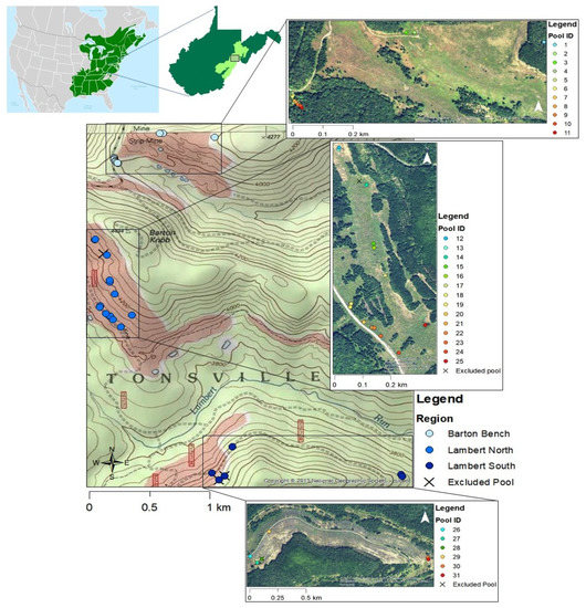
Figure 1.
Map displaying study area in Randolph County, WV, in the Greenbrier District of Monongahela National Forest. Circles represent locations of sampled created vernal pools designated by region. Pools at Barton Bench were created in 2011 (n = 11), Lambert North pools were created in 2013 (n = 14), and Lambert South pools were created in 2014 (n = 6). State map displays Monongahela National Forest and the general area of sampling with a black box. USA topo map accessed through ESRI © 2013 National Geographic Society, i-cubed; world imagery source: Esri, DigitalGlobe, GeoEye, Earthstar Geographics, CNES/Airbus DS, USDA, USGS, AeroGRID, IGN, and the GIS User Community. Spotted Salamander range map from Cephas https://commons.wikimedia.org/wiki/File:Ambystoma_maculatum_map.svg (accessed on 6 January 2023).
2.2. Field Sampling
Using dipnets and seines, we sampled spotted salamander larvae in 34 created vernal pools: 22 in both years, 8 in 2015, and 4 in 2016. By region, this included 11 pools in Barton Bench, 14 pools in Lambert North, and 6 pools in Lambert South. We caught 14–30 (mean = 20.73, SE = 0.31) larvae per pool per sampling year. Vernal pools were sampled once per year between May and June [24]. Upon capture, we collected tail clips (<1 cm), which were stored fully immersed in 100% ethanol in 1.5 mL microcentrifuge tubes until later DNA extraction. Salamanders were released after all larvae from the pool were processed.
We collected data on conditions at each pool to investigate how environmental variables influenced spotted salamander population genetics. We measured the diameter of each pool using the average of perpendicular transects [25]. We used the line intercept method to measure cover within the pool along the same two transects used for diameter [17,26]. Cover within the pool (pool cover) was considered any form of refuge within the pool, including rocks, coarse woody debris, and vegetation. In addition to looking at all pool cover, we examined a subset of the pool cover: grass, sedge, cattail, and rush (GSCR) within the pool. Proportional cover for pool cover and GSCR was calculated as the total length of cover types divided by the length of transects at the pool [17]. Canopy cover was measured using a spherical densiometer every 1.5 m along transects [25]. Predator presence was quantified by presence/absence rating (0/1) when the following were caught in nets or observed in pools: eastern newts (Notophthalmus viridescens), diving beetle (Dytiscidae) larvae, and dragonfly (Odonata) larvae. Pools could have a rating of 0, meaning none were present, to 3, where all three were observed in the pool [25]. Pool age was calculated by sampling year minus creation year. The geographic location and age of the pool are not independent because pools created each year were all made in the same area.
2.3. Genetic Analysis
We extracted DNA from the tail clips of spotted salamander larvae using Promega Wizard® SV 96 Genomic DNA Purification System kits. Every DNA sample was tested using a nano spectrophotometer and standardized to a concentration of 15 ng/μL. We used eight microsatellite markers (D184, D287, C151, D315, D226, D49, D328, D203) [27] and three universal primers to multiplex microsatellite loci (Table S1; Supplement S1) [28]. For pools sampled in both years, we tested the annual variation of allele frequencies using exact G test in GENEPOP with sequential Bonferroni correction (α = 0.05). If there was no difference between years, data from both years were combined to increase the sample size for that pool (N = 17 pools; Table S2). If pools differed from one year to the next, only the year with a higher sample size was retained (N = 5 pools). We removed 3 pools with fewer than 10 individuals (Table S2).
The initial analysis tested for excess homozygotes, scoring error, allele dropout, and null alleles in MICRO-CHECKER [29]. To avoid bias associated with relatedness in free-moving larvae in pools, we removed full siblings in COLONY [30,31]. In COLONY, we set male and female mating to polygamous without inbreeding. We conducted a medium run with full likelihood and omitted a sibship prior. We ran the analysis in duplicate. When full siblings were detected in both runs, only one of the siblings was kept for subsequent analysis. We tested for the Hardy–Weinberg equilibrium and linkage disequilibrium using GENEPOP with 10,000 iterations followed by sequential Bonferroni correction (α = 0.05) [32].
2.4. Population Structure
We tested the number of genetically distinct populations in the study area using STRUCTURE 2.3.4 [33]. We created three a priori sampling units (region) by grouping pools that were geographically proximate and created at the same time (Barton Bench, Lambert North, Lambert South). We ran STRUCTURE with 150,000 burn-ins and 150,000 reps with the locprior model with admixture. We hypothesized that there were no more than 10 populations based on the initial analysis. We conducted ten runs for each value of K = 1–10. We used STRUCTURE HARVESTER [34] to determine optimal K based on peak average Ln Pr(X|K) [33]. After an initial run to explore the highest level of structure, we used the model with the highest probability. We ran a subsequent hierarchical analysis in each group to examine substructure. In the subsequent analyses, we used the same parameters, except we set the burn-in period and reps to 100,000 and K to the number of pools in each region.
To confirm groupings indicated by STRUCTURE, we ran an Analysis of Molecular Variance (AMOVA) in Arlequin ver. 3.0 [35] with 10,000 permutations (α = 0.05). Pairwise differences between pools were calculated using genetic differentiation (FST) between individual pools using FSTAT with 10,000 iterations and regular Bonferroni correction (α = 0.05) [36]. We tested for recent bottlenecks using BOTTLENECK software with a two-phase mutation model, a variance of 12, 95% single-step mutations, and 1000 iterations, for the sign test, Wilcoxon sign rank test, and mode-shift test (α = 0.05) [37].
2.5. Effective Number of Breeders and Genetic Diversity
To determine how pool creation year, sample size, and local environmental traits impacted genetic diversity, we examined the following at pool level: Nb, HE, AR, and relatedness. We used FSTAT with 10,000 iterations to calculate HE and AR (based on the minimum sample size of 10 individuals [36]. We measured Nb using COLONY [10,38]. We calculated relatedness within pools by mean within-population pairwise values using GenAlEx [39,40] and the Queller and Goodnight estimator [41]. We tested for differences between regions using the Kruskal–Wallis rank sum test followed by Dunn’s test (α = 0.05; package ‘dunn.test’) [42] due to non-normally distributed data.
2.6. Environmental Factors
Environmental analysis was conducted in R [43]. To explore how environmental factors influenced genetic characteristics, we compared linear regression models (α = 0.05) and determined the best environmental predictors for Nb, within-pool relatedness, HE, and AR using Akaike information criterion (AICc) (package ‘AICcmodavg’) [44,45]. We examined deviance explained by each model (package ‘BiodiversityR’) [46]. Environmental predictors included in the analysis were: age of pool, diameter of pool, pool cover, GSCR, canopy cover, and predator presence. Because pool age is linked to region, we used age in the regression models, which incorporates additional variation because age changed from sample year one to sample year two; except for relatedness because the region was a stronger predictor. By including sample size, we could investigate if environmental conditions were stronger predictors than sample size alone, therefore more accurately determining habitat influence. For regression models with environmental predictors, we excluded two pools that were outliers to prevent skewing the data based on a single data point: Barton Bench pool 1 (only from Nb regressions) and Lambert South pool 30 (Grubbs test p < 0.001; package ‘outliers’) [47].
3. Results
The final dataset for the genetic analysis included 795 spotted salamander samples from 31 pools (Barton Bench = 351, Lambert North = 350, Lambert South = 94): 14 based on one year of sampling and 17 based on two years of sampling (Table S2). Results from MICROCHECKER led us to drop three loci (D315, D203, D328) due to null alleles in 43–68% of pools sampled. This left five remaining microsatellite loci (Table S1). All pools were in Hardy–Weinberg Equilibrium and linkage equilibrium after sequential Bonferroni correction (p > 0.05).
3.1. Population Structure
At the highest level, the Bayesian clustering algorithm of STRUCTURE found the model with the highest probability was K = 1, grouping all the pools from all regions into a single population (Figure S1). However, when examined further, the barplot reflected a cline across the three regions that we had grouped a priori by proximity and by year of creation (Figure 2a). The cline depicted Barton Bench and Lambert South as genetically distinct ends with individuals in Lambert North displaying high admixture derived from the other populations. After the hierarchical STRUCTURE analysis by region, the highest probability models suggested K = 1 for Barton Bench, K = 3 for Lambert North, and K = 2 for Lambert South (Figure 2b–d and Figure S2).
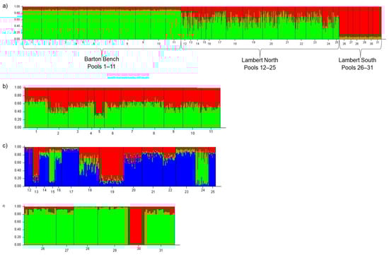
Figure 2.
STRUCTURE barplots most likely displaying K. Colors indicate the individual membership coefficients for each cluster. Numbers reflect pool IDs. (a) Barplot for entire study area including all three regions (Barton Bench, Lambert North, Lambert South); most likely K = 1. (Presenting barplot K = 2 to visually display the allele proportions reflecting a cline across regions.) (b) Barplot for pools in Barton Bench region created in 2011; most likely K = 1. [Presenting barplot K = 2 to visually display the allele proportions reflect K = 1] (c) Barplot for pools in Lambert North region created in 2013; most likely K = 3. (d) Barplot for pools in Lambert South region created in 2014; most likely K = 2.
The AMOVA confirmed significant genetic differentiation between the three a priori grouped regions (p = 0.0006), among the pools within the regions (p < 0.0001), and within pools (p < 0.0001). Pairwise FST across pools ranged from 0–0.17 (mean = 0.03, SE = 0.001) (Table S3, Figure S3). There were 152 pairwise comparisons (33%) that were significantly differentiated after Bonferroni correction, 65 had moderate differentiation (FST = 0.05–0.10), and 22 were highly differentiated (FST > 0.10) (Table S3, Figure S3). Moderate and high differentiation were observed at pools in Lambert North and Lambert South. There was a distinct increase in differentiation from Barton Bench to Lambert North to Lambert South. Pairwise differentiation was highest in the most recently created region, Lambert South (Figure S3). There was some differentiation in Lambert North and little to none in Barton Bench. We analyzed the three regions separately in BOTTLENECK and none of them exhibited recent bottlenecks (p > 0.05).
3.2. Effective Number of Breeders and Genetic Diversity
Effective number of breeders was higher in the older pools at Barton Bench and Lambert North than in the newest pools at Lambert South (p ≤ 0.02; Figure 3). Effective number of breeders ranged from 4–18 at Lambert South, 7–26 at Lambert North, and 13–90 at Barton Bench averaging 12.00, 18.86, and 28.45 respectively (Table S4). Relatedness, HE, and AR were not different among regions (p > 0.05) (Tables S4 and S5, Figure 3). Relatedness ranged from 0–0.49 across all regions, averaging 0.04 in Barton Bench, 0.05 in Lambert North, and 0.15 in Lambert South. Expected heterozygosity ranged from 0.64–0.83 across all regions, averaging 0.79 at Barton Bench, 0.80 at Lambert North, and 0.77 at Lambert South. Allelic richness ranged from 3.00–7.39 across all regions, averaging 6.51 in Barton Bench, 6.63 in Lambert North, and 5.89 in Lambert South (Tables S4 and S5, Figure 3).
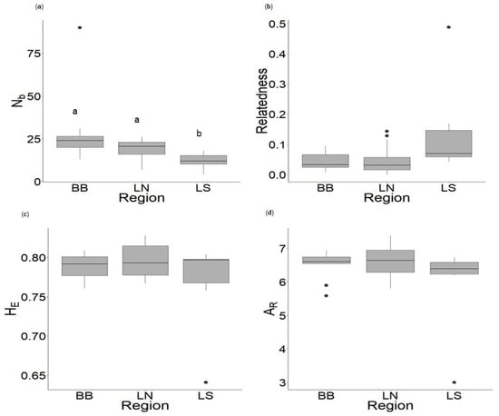
Figure 3.
Boxplots displaying ranges in (a) effective number of breeders (Nb), (b) relatedness, (c) expected heterozygosity (HE), and (d) allelic richness (AR) for spotted salamanders (Ambystoma maculatum) across regions: Barton Bench (BB; N = 11), Lambert North (LN; N = 14), Lambert South (LS; N = 6). Letters indicate significant differences between regions (Dunn’s Test p < 0.05).
3.3. Environmental Factors
We controlled sample size by including it as a predictor in regression models to account for its positive correlation with Nb, HE, and AR, and negative correlation with relatedness. The effective number of breeders was significantly correlated with multiple environmental predictors. The best model predicting Nb included age of pool + GSCR + diameter of pool + sample size within pool (adj r2 = 0.68, F [4,24] = 15.97, p < 0.0001) (Table 1, Table 2 and Table 3). This model explained 73% of the variance in the data and was given 70% of the weight of all models in AIC, but not all coefficients were different from zero (Table 1, Table 2 and Table 3). All predictors of the top model had positive relationships with Nb (Figure 4). Two models had ΔAIC less than seven indicating they could be competing models. The model pool diameter + canopy cover + sample size was weighted 21% and explained 67% of the deviance (Table 1 and Table 3). These predictors all had positive relationships with Nb and estimates significantly different from zero (Table 1, Figure S4). The full model, which included predictors from the top two models and predator presence, had ΔAIC = 4.57 indicating it could also be significant, but it was only weighted at 7% (Table 1 and Table 3, Figure S4).

Table 1.
Hypothesized models predicting effective number of breeders of spotted salamanders (Ambystoma maculatum). Predictors include age of pool; cover of grass, sedge, cattail, and rush within pool (GSCR); diameter of pool; sample size within the pool; canopy cover; predator presence; and the null ~1. ΔAICc = change in AIC corrected for small sample size; wi = weight of the model; asterisks indicate when all predictors in a model had an estimate and 95% CI interval not overlapping zero.
Table 2.
Coefficients for the top model predicting effective number of breeders for spotted salamanders (Ambystoma maculatum): y = age of pool + GSCR (grass, sedge, cattail, rush coverage) + diameter of pool + sample size within pool.
Table 3.
Summary statistics of predictors included in spotted salamander (Ambystoma maculatum) population genetics models, including the age of pool; canopy cover; diameter (m) of pool; cover of grass, sedge, cattail, and rush within pool (GSCR); cover by any form of refuge within the pool such as vegetation, rocks, and coarse woody debris (pool cover); predator presence; and sample size per pool.
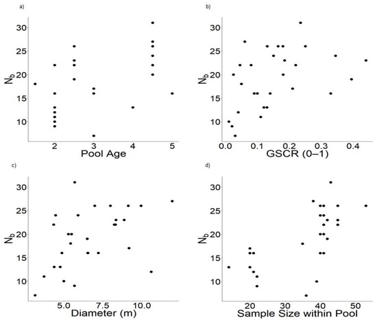
Figure 4.
Biplots displaying the relationship between Nb and predictors from the most robust model including: (a) age of pool, (b) GSCR (0–1) (grass, sedge, cattail, and rush coverage within pool), (c) diameter (m) of pool, and (d) sample size within the pool. Some ages are in-between years due to combining samples collected over two years.
Relatedness had multiple competing models with ΔAIC less than two. These included models with the predictor’s pool cover, sample size, GSCR, region, and pool diameter (Table 4). In every model, predictors had negative relationships with relatedness (Table 4 and Table 5, Figure 5). The top model was pool cover + sample size, which was weighted 27% and explained 32% of the deviance (adj r2 = 0.27, F [2,27] = 6.26, p = 0.006; Table 5, Figure 5). The second strongest model was GSCR + sample size with ΔAIC less than one.
Table 4.
Hypothesized models predicting relatedness for spotted salamanders (Ambystoma maculatum). Predictors include pool cover which consists of any form of refuge such as vegetation, rocks, coarse woody debris; sample size within the pool; cover of grass, sedge, cattail, and rush within the pool (GSCR); region; diameter of the pool; predator presence; and the null ~1. ΔAICc = change in AIC corrected for small sample size; wi = weight of the model; asterisks indicate when all predictors in a model had an estimate and 95% CI interval not overlapping zero.
Table 5.
Coefficients for the top model predicting relatedness for spotted salamanders (Ambystoma maculatum): y = pool cover + sample size within the pool.
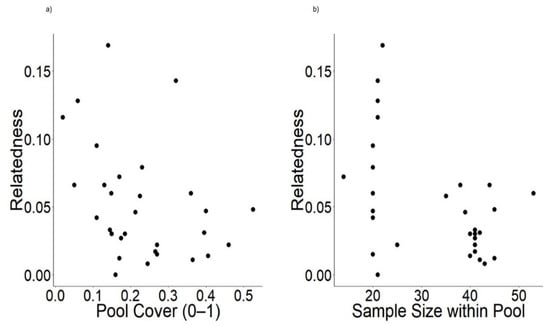
Figure 5.
Biplots displaying the relationship between relatedness and predictors from the strongest model including: (a) GSCR (0–1) (grass, sedge, cattail, and rush coverage within pool) and (b) sample size within pool.
The only significant regression model for HE was pool cover + sample size (y = 0.77 + 0.05 pool cover + 0.0005 sample size within pool: adj r2 = 0.16, F [2,27] = 3.68, p = 0.04). Both predictors had positive relationships with HE (Figure S5). The coefficients were not significantly different from zero (p > 0.05), and individually, these predictors were not significant. Allelic richness had no significant environmental predictors (p > 0.05).
4. Discussion
We investigated the genetic diversity of spotted salamander larvae in 31 created vernal pools in the Central Appalachians. As expected, older pools had lower genetic differentiation and higher Nb. Larger pools with greater vegetative cover had higher Nb. Greater vegetative cover also had a negative association with relatedness. Finally, there was weak evidence for a positive relationship between pool cover and HE.
4.1. Population Structure
Although the study area spanned 5 km, it was a panmictic single population with a cline in population structure from Barton Bench to Lambert North to Lambert South. This suggests that there is migration from Barton Bench and Lambert South into Lambert North, which was between the other regions both geographically and in age. Barton Bench and Lambert South had the oldest and youngest created pools, respectively, and were furthest apart geographically. Individual spotted salamanders have been documented traveling maximum distances of 467 m from breeding ponds; however, this species exhibits genetic connectivity among pools within distances up to 17 km [48,49]. It is possible that migrants from the other two regions into Lambert North helped increase population size, resulting in the highest genetic diversity, and similar levels of Nb and relatedness to Barton Bench, despite Lambert North being two years younger.
Genetic differentiation between regions was low, indicating movement and migration among regions and no major obstructions to gene flow. Several pairwise comparisons were significant, and some were highly differentiated at pools in Lambert North and Lambert South. Genetic differentiation between some pools might indicate that it takes longer than 1–3 years for colonizers to establish and disperse among pools. These results are consistent with research conducted in Maine, where spotted salamander breeding effort and reproductive success were variable for six years after pool creation [15]. In tiger salamanders, newly colonized wetlands had greater genetic differentiation than established populations [14]. Additionally, female spotted salamanders do not reach sexual maturity for 3–5 years, meaning it would take at least as long to measure the reproductive success of offspring produced in the created pools [50,51]. The pools in our study were colonized as early as the first breeding season after pool creation, reflecting spotted salamanders’ rapid colonizing ability. This was also seen in created pools in North Carolina, where spotted salamanders colonized 9 out of 10 pools the first year of creation, the same rate as natural pools sampled [18]. However, determining long-term success requires monitoring for longer than three years, even when breeding is evident in the first year of creation.
We expected to detect a bottleneck as the result of a founder effect in all regions, where the low number of colonizing individuals brings limited genetic diversity to the newly created pools but did not detect any bottlenecks. A possible founder effect in the younger pools at Lambert South was evident from the higher genetic differentiation of these pools compared to the older pools [14]. Additionally, salamanders in pools at Lambert South had the lowest Nb, HE, and AR, and the highest relatedness. However, the latter three were not significantly different from other regions. Only Nb was significantly different among regions, and only at Lambert South. In such newly created pools, a smaller breeding population, lower genetic diversity, and higher relatedness may indicate that these breeding pools were exhibiting signs of a founder effect despite lack of significance in bottleneck tests. The ability to detect a bottleneck could have been limited due to the low number of loci, immigration among regions, and size of the source population [52,53,54].
4.2. Effective Number of Breeders and Genetic Diversity
The effective number of breeders was highest in the oldest pools (4–5 years old) and lowest in the newest pools (1–2 years old). Only Barton Bench had Nb values comparable to those of an established spotted salamander population in Maine across 19 pools [55]. Even the maximum Nb for the regions with younger pools was lower than the range of the population in Maine [55]. This indicates Nb increased within a couple of years in these created vernal pools and shows potential for populations inhabiting created pools to establish breeding populations of a similar size to those of natural pools. Additionally, in three created pools in Maine, the abundance of breeding spotted salamanders increased 3–6 years after construction [15]. Spotted salamanders sampled across 26 natural pools in Connecticut and Massachusetts had an average Ne of 570 [56]. Based on the Nb/Ne ratios of Allegheny Mountain dusky salamanders (Desmognathus ochrophaeus) (0.734) [11], we can estimate that our maximum Nb = 90 at Barton Bench would be roughly equivalent to Ne = 123, lower than the established population in Connecticut and Massachusetts [56]. In all regions, genetic diversity (HE and AR) was similar to breeding populations in Maine, Connecticut, and Massachusetts, except for the low AR of pool 30 in Lambert South [55,56]. Genetic diversity did not differ by pool age. Relatedness, HE, and AR were similar across regions despite expectations that HE and AR would increase, and relatedness would decrease over time as breeding populations became established. More time may be necessary to detect changes in genetic diversity in colonizing populations. However, in tiger salamanders, population age, based on three years of data, was not a significant predictor for AR [14]. Because genetic diversity in our pools was similar to established natural populations [55,56], it is possible that the rapid colonization of our pools resulted in natural diversity levels.
4.3. Environmental Factors
Habitat quality can impact the population genetics of amphibians [12,13]. We found that multiple habitat characteristics influenced Nb, including positive associations with pool age, diameter, and GSCR. In addition to differences in Nb among regions, age was a top predictor for Nb, indicating that time since creation impacted Nb. The changes in Nb with pool age highlight the importance of monitoring populations over time. Larger pools (up to 11.94 m diameter) had higher Nb, indicating that larger pools may attract more breeders. Others have found that larger pools had higher spotted salamander occupancy, more egg masses, and higher larval survival rates [17,18,57,58]. Similarly, California tiger salamanders (Ambystoma californiense) had higher Ne in larger vernal pools [38]. Tiger salamander wetland colonization was positively related to wetland area [59]. Larger wetlands also had higher immigration rates for marbled salamanders (Ambystoma opacum) [60]. Larger wetlands produced lower genetic differentiation in tiger salamanders, potentially indicating higher gene flow [14]. Salamanders may show a preference for larger breeding pools, or higher colonization rates may be a product of the target effect, where salamanders are more likely to encounter larger pools during spring migrations to breeding sites [59,61]. These data indicate larger pools can support successful breeding populations [14]. Additionally, larger pools in our study system produced spotted salamander larvae with lower stress hormone levels [25]. It is important to note that the created pools in this study were smaller in size than natural pools with breeding spotted salamander populations in Maine, which had average diameters of 15–25 m (unpublished data [48]), compared to the average diameter of 7 m in this study.
The top models indicate that GSCR and canopy cover are positive predictors of Nb. Greater pool cover and vegetation cover were also negatively associated with relatedness within pools. This could confirm expectations that pools with higher coverage of GSCR would provide a more suitable habitat for egg mass deposition and larval refuge from predators [62]. Higher availability of GSCR in a pool may attract more breeding adults or provide more surface area for egg masses. Spotted salamander egg mass density and larval survival was higher in breeding pools with greater vegetative cover [17,58,63]. Canopy cover is more difficult to interpret because only 7 of the 31 pools had any canopy cover and they were all in the Barton Bench region. The positive relationship between canopy cover and Nb may reflect higher levels of Nb in Barton Bench due to pool age. However, spotted salamanders oviposited more egg masses in pools with surrounding forest cover and avoided clear-cut forests [19,20,21]. Pools with greater canopy cover also had a higher density of spotted salamander larvae [64]. Therefore, canopy cover could be an important factor for spotted salamander breeding habitat.
There is weak evidence that as pool cover increased, HE increased. This may be related to the higher reproductive effort in pools with more vegetation [17,63]. We did not find an effect of pool size on AR or HE, which was also true for the California tiger salamander in vernal pools [38]. Pond size negatively impacted the allelic diversity of California tiger salamanders in deeper, permanent, artificial pools [38]. Conversely, AR of tiger salamanders in Illinois increased with wetland area [14].
An inherent difficulty of a newly created habitat is the dependency on migration and colonization. There were pools in Lambert North and Lambert South, with larvae present in 2015 but not in 2016. At one pool in Lambert North, we caught 22 larvae in 2015 but none in 2016. After removing full siblings, only three individuals remained with Nb = 4. Lambert North pool 25 was surprising because after successfully catching 21 larvae in two person-hours in 2015, we only found 2 larvae in 2016, despite previously observing 12 egg masses and sampling the entire area of the pool multiple times over two person-hours. This pool had Nb = 12, lower than the region’s average (Nb = 19). Lambert South pool 30 was an extreme among our sampled pools, with the lowest Nb, highest relatedness, and lowest genetic diversity (Lambert South region means in parentheses): Nb = 4 (vs. 12), relatedness = 0.49 (vs. 0.13), HE = 0.64 (vs. 0.77), and AR = 3 (vs. 5.89). These unique pools demonstrate the stochastic nature of newly colonized pools, as the presence of breeding spotted salamanders for one year does not indicate an established population. Long-term monitoring is important to determine the viability of populations in created pools because it may take many years for a population to establish [15].
5. Conclusions
Time since pool creation and habitat quality relate to spotted salamanders’ genetic diversity and differentiation in created vernal pools. Pools were colonized quickly by spotted salamanders, and Nb increased as soon as 4–5 years after habitat creation. These older pools also had low genetic differentiation and no bottlenecks, indicating an establishing breeding population. Vegetation cover within the pool (GSCR) and pool diameter were important predictors of Nb, indicating it would be valuable to incorporate vegetative cover within created pools to provide oviposition sites and refuge for larvae. Future vernal pool creation would benefit from larger vernal pools, and future research should determine the ideal pool size to attract and support spotted salamander breeding populations. At our study site, there should be continued monitoring to determine if Nb increases and genetic differentiation decreases with time since creation at the youngest pools. In general, this work highlights that genetic analyses can be used to help assess the success of colonization, and combined with environmental data, help inform future site selection and creation of vernal pools. Moreover, long-term monitoring is essential to track changes and determine if created pools sustain viable breeding populations.
Supplementary Materials
The following supporting information can be downloaded at: https://www.mdpi.com/article/10.3390/d15020124/s1. Table S1: Details of microsatellites with PCR conditions. Microsatellite loci are from Julian et al. (2003) [27]. Universal primers are from Blacket et al. (2012) [28]. *Loci excluded from analysis; Table S2: List of all pools sampled specifying which were included in analysis. Regions include Barton Bench (BB), Lambert North (LN), and Lambert South (LS). Sample size is the number of spotted salamander (Ambystoma maculatum) larvae per pool included in analysis. Years sampled were 2015, 2016, or both. Years combined indicates whether data from two years were combined: yes Y, no N, or N/A if only sampled one year. Sample year included is bolded for pools with only one year of sampling included in analysis. Final pool sample size included 31 pools: 14 based on one year of sampling and 17 based on two years of sampling; Table S3: Fst table displaying Fst values in the top half and p-values in the bottom half. Significant values are bolded. Pool ID listed by region: Barton Bench 1–11 (BB), Lambert North 12–25 (LN), and Lambert South 26–31 (LS); Table S4: Summary statistics of effective number of breeders (Nb), relatedness (), expected heterozygosity (HE), and allelic richness (AR) for spotted salamanders (Ambystoma maculatum) separated by region: Barton Bench (BB), Lambert North (LN), and Lambert South (LS); Table S5 Pool level values of effective number of breeders (Nb), relatedness, expected heterozygosity (HE), and allelic richness (AR) for spotted salamanders (Ambystoma maculatum) with region indicated as Barton Bench (BB), Lambert North (LN), and Lambert South (LS); Figure S1: Map displaying the Barton Bench study region. Circles represent sampled created vernal pool locations designated by individual pool ID. World imagery source: Esri, DigitalGlobe, GeoEye, Earthstar Geographics, CNES/Airbus DS, USDA, USGS, AeroGRID, IGN, and the GIS User Community; Figure S2: Map displaying the Lambert North study region. Circles represent sampled created vernal pool locations designated by individual pool ID. World imagery source: Esri, DigitalGlobe, GeoEye, Earthstar Geographics, CNES/Airbus DS, USDA, USGS, AeroGRID, IGN, and the GIS User Community; Figure S3: Map displaying the Lambert South study region. Circles represent sampled created vernal pool locations designated by individual pool ID. World imagery source: Esri, DigitalGlobe, GeoEye, Earthstar Geographics, CNES/Airbus DS, USDA, USGS, AeroGRID, IGN, and the GIS User Community; Figure S4: Plot of most likely number of spotted salamander (Ambystoma maculatum) populations (K) across the entire study area (encompassing all three regions together) by the mean of estimated ln probability of the data. Analysis included all regions grouped together using 5 microsatellite loci run on STRUCTURE with graph produced by STRUCTURE HARVESTER; Figure S5: Plot of most likely number of spotted salamander (Ambystoma maculatum) populations (K) by the mean of estimated Ln probability of the data for regions (a) Barton Bench (b) Lambert North and (c) Lambert South. Analysis included 5 microsatellite loci run on STRUCTURE with graph produced by STRUCTURE HARVESTER
Author Contributions
A.R.M., S.S.C. and J.T.A. designed the study; A.R.M. and J.T.A. secured funding; A.R.M. collected field data and lab analysis with input from S.S.C.; A.R.M. conducted data analysis with input from S.S.C. and A.B.W.; A.R.M. wrote the manuscript with significant contributions from all authors. All authors have read and agreed to the published version of the manuscript.
Funding
This research was funded by the U.S. Forest Service, Natural Resources Conservation Service, National Science Foundation (01A-1458952), West Virginia University Natural History Museum, National Institute of Food and Agriculture McStennis Project WVA00812 and Hatch Project WVA00690, The Explorers Club Washington Group, Society of Wetland Scientists, Society of Wetland Scientists South Atlantic Chapter, West Virginia University Stitzel Graduate Enhancement Fund, and Richard and Lois Bowman.
Institutional Review Board Statement
This study complied with the relevant laws and institutional guidelines. This study was approved by West Virginia University’s Institutional Animal Care and Use Committee (15-0409.3), the U.S. Forest Service, and the West Virginia Division of Natural Resources (Scientific Collecting Permit 2015.133, 2016.205).
Data Availability Statement
The data presented in this study are available on request from the corresponding author. The data are not publicly available due to privacy concerns.
Acknowledgments
We thank Jessi Rouda, Jonathan Strickland, Adam Bucher, John Millikin, Lauren Schumacher, and Meghan Jensen for field and lab assistance. We also thank the West Virginia Division of Natural Resources and the Ruby Distinguished Doctoral Fellowship Program.
Conflicts of Interest
The authors declare that they have no known competing financial interests or personal relationships that could have appeared to influence the work reported in this paper.
References
- Calhoun, A.J.K.; Mushet, D.M.; Bell, K.P.; Boix, D.; Fitzsimons, J.A.; Isselin-Nondedeu, F. Temporary wetlands: Challenges and solutions to conserving a ‘disappearing’ ecosystem. Biol. Conserv. 2017, 211, 3–11. [Google Scholar] [CrossRef]
- Mushet, D.M.; Calhoun, A.J.K.; Alexander, L.C.; Cohen, M.J.; DeKeyser, E.S.; Fowler, L.; Lane, C.R.; Lang, M.W.; Rains, M.C.; Walls, S.C. Geographically isolated wetlands: Rethinking a misnomer. Wetlands 2015, 35, 423–431. [Google Scholar] [CrossRef]
- DiBello, F.J.; Calhoun, A.J.; Morgan, D.E.; Shearin, A.F. Efficiency and detection accuracy using print and digital stereo aerial photography for remotely mapping vernal pools in New England landscapes. Wetlands 2016, 36, 505–514. [Google Scholar] [CrossRef]
- Calhoun, A.J.K.; Arrigoni, J.; Brooks, R.P.; Hunter, M.L.; Richter, S.C. Creating successful vernal pools: A literature review and advice for practitioners. Wetlands 2014, 34, 1027–1038. [Google Scholar] [CrossRef]
- Spielman, D.; Brook, B.W.; Frankham, R. Most species are not driven to extinction before genetic factors impact them. Proc. Natl. Acad. Sci. USA 2004, 101, 15261–15264. [Google Scholar] [CrossRef]
- Frankham, R. Genetics and extinction. Biol. Conserv. 2005, 126, 131–140. [Google Scholar] [CrossRef]
- Beebee, T.J.C. Conservation genetics of amphibians. Heredity 2005, 95, 423–427. [Google Scholar] [CrossRef]
- Reed, D.H.; Frankham, R. Correlation between fitness and genetic diversity. Conserv. Biol. 2003, 17, 230–237. [Google Scholar] [CrossRef]
- Ruzzante, D.E.; McCracken, G.R.; Parmelee, S.; Hill, K.; Corrigan, A.; MacMillan, J.L.; Walde, S.J. Effective number of breeders, effective population size and their relationship with census size in an iteroparous species, Salvelinus fontinalis. Proc. R. Soc. B 2016, 283, 20152601. [Google Scholar] [CrossRef]
- Wang, J. A new method for estimating effective population sizes from a single sample of multilocus genotypes. Mol. Ecol. 2009, 18, 2148–2164. [Google Scholar] [CrossRef]
- Waples, R.S.; Luikart, G.; Faulker, J.R.; Tallmon, D.A. Simple life-history traits explain key effective population size ratios across diverse taxa. Proc. R. Soc. B 2013, 280, 20131339. [Google Scholar] [CrossRef]
- McKee, A.M.; Maerz, J.C.; Smith, L.L.; Glenn, T.C. Habitat predictors of genetic diversity for two sympatric wetland-breeding amphibian species. Ecol. Evol. 2017, 7, 6271–6283. [Google Scholar] [CrossRef]
- Costanzi, J.-M.; Mège, P.; Boissinot, A.; Isselin-Nondedeu, F.; Guérin, S.; Lourdais, O.; Trochet, A.; Le Petitcorps, Q.; Legrand, A.; Varenne, F.; et al. Agricultural landscapes and the Loire River influence the genetic structure of the Marbled Newt in Western France. Sci. Rep. 2018, 8, 14177. [Google Scholar] [CrossRef]
- Cosentino, B.J.; Phillips, C.A.; Schooley, R.L.; Lowe, W.H.; Douglas, M.R. Linking extinction-colonization dynamics to genetic structure in a salamander metapopulation. Proc. R. Soc. B 2012, 279, 1575–1582. [Google Scholar] [CrossRef]
- Vasconcelos, D.; Calhoun, A.J.K. Monitoring created seasonal pools for functional success: A six-year case study of amphibian responses, Sears Island, Maine, USA. Wetlands 2006, 26, 992–1003. [Google Scholar] [CrossRef]
- Denton, R.D.; Richter, S.C. Amphibian communities in natural and constructed ridge top wetlands with implications for wetland construction. J. Wildl. Manag. 2013, 77, 886–896. [Google Scholar] [CrossRef]
- Egan, R.S.; Paton, P.W.C. Within-pond parameters affecting oviposition by wood frogs and spotted salamanders. Wetlands 2004, 24, 1–13. [Google Scholar] [CrossRef]
- Petranka, J.W.; Kennedy, C.A.; Murray, S.S. Response of amphibians to restoration of a southern Appalachian wetland: A long-term analysis of community dynamics. Wetlands 2003, 23, 1030–1042. [Google Scholar] [CrossRef]
- Skidds, D.E.; Golet, F.C.; Paton, P.W.; Mitchell, J.C. Habitat correlates of reproductive effort in wood frogs and spotted salamanders in an urbanizing watershed. J. Herpetol. 2007, 41, 439–451. [Google Scholar] [CrossRef]
- Felix, Z.I.; Wang, Y.; Schweitzer, C.J. Effects of experimental canopy manipulation on amphibian egg deposition. J. Wildl. Manag. 2010, 74, 496–503. [Google Scholar] [CrossRef]
- Scheffers, B.R.; Furman, B.L.S.; Evans, J.P. Salamanders continue to breed in ephemeral ponds following the removal of surrounding terrestrial habitat. Herpetol. Conserv. Biol. 2013, 8, 715–723. [Google Scholar]
- Petranka, J.W.; Murray, S.S.; Kennedy, C.A. Responses of amphibians to restoration of a southern Appalachian wetland: Perturbations confound post-restoration assessment. Wetlands 2003, 23, 278–290. [Google Scholar] [CrossRef]
- Canty, J.L. Weatherbase. Available online: http://weatherbase.com (accessed on 22 June 2018).
- Millikin, A.R.; Davis, D.R.; Brown, D.J.; Woodley, S.K.; Coster, S.; Welsh, A.; Kerby, J.L.; Anderson, J.T. Prevalence of ranavirus in spotted salamander larvae from created vernal pools in West Virginia, USA. J. Wildl. Dis. 2023. [Google Scholar] [CrossRef]
- Millikin, A.R.; Woodley, S.K.; Davis, D.R.; Anderson, J.T. Habitat characteristics in created vernal pools impact spotted salamander water-borne corticosterone levels. Wetlands 2019, 39, 803–814. [Google Scholar] [CrossRef]
- Barbour, M.G.; Burk, J.H.; Pitts, W.D.; Gilliam, F.S.; Schwartz, M.W. Terrestrial Plant Ecology; Benjamin and Cummings: Menlo Park, CA, USA, 1999. [Google Scholar]
- Julian, S.E.; King, T.L.; Savage, W.K. Isolation and characterization of novel tetranucleotide microsatellite DNA markers for the spotted salamander, Ambystoma maculatum. Mol. Ecol. Resour. 2003, 3, 7–9. [Google Scholar] [CrossRef]
- Blacket, M.J.; Robin, C.; Good, R.T.; Lee, S.F.; Miller, A.D. Universal primers for fluorescent labeling of PCR fragments—An efficient and cost-effective approach to genotyping by fluorescence. Mol. Ecol. Resour. 2012, 12, 456–463. [Google Scholar] [CrossRef]
- Van Oosterhout, C.; Hutchinson, W.F.; Wills, D.P.; Shipley, P. MICRO-CHECKER: Software for identifying and correcting genotyping errors in microsatellite data. Mol. Ecol. Resour. 2004, 4, 535–538. [Google Scholar] [CrossRef]
- Wang, J. Sibship reconstruction from genetic data with typing errors. Genetics 2004, 166, 1963–1979. [Google Scholar] [CrossRef]
- Goldberg, C.S.; Waits, L.P. Quantification and reduction of bias from sampling larvae to infer population and landscape genetic structure. Mol. Ecol. Resour. 2010, 10, 304–313. [Google Scholar] [CrossRef]
- Raymond, M.; Rousset, F. GENEPOP (version 1.2): Population genetics software for exact tests and ecumenicism. J. Hered. 1995, 86, 248–249. [Google Scholar] [CrossRef]
- Pritchard, J.K.; Stephens, M.; Donnelly, P. Inference of population structure using multilocus genotype data. Genetics 2000, 155, 945–959. [Google Scholar] [CrossRef]
- Earl, D.A.; von Holdt, B.M. STRUCTURE HARVESTER: A website and program for visualizing STRUCTURE output and implementing the Evanno method. Conserv. Genet. Resour. 2012, 4, 359–361. [Google Scholar] [CrossRef]
- Excoffier, L.; Laval, G.; Schneider, S. Arlequin (version 3.0): An integrated software package for population genetics data analysis. Evol. Bioinform. Online 2005, 1, 47–50. [Google Scholar] [CrossRef]
- Goudet, J. FSTAT (Version 1.2): A computer program to calculate F-statistics. J. Hered. 1995, 86, 485–486. [Google Scholar] [CrossRef]
- Piry, S.; Luikart, G.; Cornuet, J.-M. BOTTLENECK: A computer program for detecting recent reductions in the effective population size using allele frequency data. J. Hered. 1999, 90, 502–503. [Google Scholar] [CrossRef]
- Wang, I.J.; Johnson, J.R.; Johnson, B.B.; Shaffer, H.B. Effective population size is strongly correlated with breeding pond size in the endangered California tiger salamander, Ambystoma californiense. Conserv. Genet. 2011, 12, 911–920. [Google Scholar] [CrossRef]
- Peakall, R.; Smouse, P.E. GENALEX 6: Genetic analysis in Excel. Population genetic software for teaching and research. Mol. Ecol. Notes 2006, 6, 288–295. [Google Scholar] [CrossRef]
- Peakall, R.; Smouse, P.E. GenAlEx 6.5: Genetic analysis in Excel. Population genetic software for teaching and research–an update. Bioinformatics 2012, 28, 2537–2539. [Google Scholar] [CrossRef]
- Queller, D.C.; Goodnight, K.F. Estimating relatedness using genetic markers. Evolution 1989, 43, 258–275. [Google Scholar] [CrossRef]
- Dinno, A. Dunn.Test: Dunn’s Test of Multiple Comparisons Using Rank Sums. R Package Version 1.3.5. 2017. Available online: https://CRAN.R-project.org/package=dunn.test (accessed on 17 July 2017).
- R Core Team. R: A Language and Environment for Statistical Computing. R Foundation for Statistical Computing, Vienna, Austria. 2017. Available online: https://www.R-project.org/ (accessed on 15 July 2017).
- Mazerolle, M.J. AICcmodavg: Model Selection and Multimodel Inference Based on (Q)AIC(c). R Package Version 2.1-1. 2017. Available online: https://cran.r-project.org/package=AICcmodavg (accessed on 15 July 2017).
- Burnham, K.P.; Anderson, D.R. Model Selection and Multimodel Inference: A Practical Information-Theoretic Approach; Springer Science & Business Media, LLC.: New York, NY, USA, 2002. [Google Scholar]
- Kindt, R.; Coe, R. Tree Diversity Analysis. A Manual and Software for Common Statistical Methods for Ecological and Biodiversity Studies; World Agroforestry Centre (ICRAF): Nairobi, Kenya, 2005; ISBN 92-9059-179-X. [Google Scholar]
- Komsta, L. Outliers: Tests for Outliers. R Package Version 0.14. 2011. Available online: https://CRAN.R-project.org/package=outliers (accessed on 20 July 2017).
- Coster, S.S.; Babbitt, K.J.; Cooper, A.; Kovach, A.I. Limited influence of local and landscape factors on finescale gene flow in two pond-breeding amphibians. Mol. Ecol. 2015, 24, 742–758. [Google Scholar] [CrossRef]
- Montieth, K.E.; Paton, P.W.C. Emigration behavior of spotted salamanders on golf courses in southern Rhode Island. J. Herpetol. 2006, 40, 195–205. [Google Scholar] [CrossRef]
- Wilbur, H.M. Propagule size, number, and dispersion pattern in Ambystoma and Asclepias. Am. Nat. 1977, 111, 43–68. [Google Scholar] [CrossRef]
- Flageole, S.; Leclair, R. Demography of a salamander (Ambystoma maculatum) population studied by skeletochronology. Can. J. Zool. 1992, 70, 740–749. [Google Scholar] [CrossRef]
- Cornuet, J.-M.; Luikart, G. Description and power analysis of two tests for detecting recent population bottlenecks from allele frequency data. Genetics 1996, 144, 2001–2014. [Google Scholar] [CrossRef] [PubMed]
- Williamson-Natesan, E.G. Comparison of methods for detecting bottlenecks from microsatellite loci. Conserv. Genet. 2005, 6, 551–562. [Google Scholar] [CrossRef]
- Peery, M.Z.; Kirby, R.; Reid, B.N.; Stoelting, R.; Doucet-Bëer, E.; Robinson, S.; Vásquez-Carrillo, C.; Pauli, J.N.; Palsbøll, P.J. Reliability of genetic bottleneck tests for detecting recent population declines. Mol. Ecol. 2012, 21, 3403–3418. [Google Scholar] [CrossRef]
- Whiteley, A.R.; McGarigal, K.; Schwartz, M.K. Pronounced differences in genetic structure despite overall ecological similarity for two Ambystoma salamanders in the same landscape. Conserv. Genet. 2014, 15, 573–591. [Google Scholar] [CrossRef]
- Richardson, J.L. Divergent landscape effects on population connectivity in two co-occurring amphibian species. Mol. Ecol. 2012, 21, 4437–4451. [Google Scholar] [CrossRef]
- Groff, L.A.; Loftin, C.S.; Calhoun, A.J.K. Predictors of breeding site occupancy by amphibians in montane landscapes. J. Wildl. Manag. 2017, 81, 269–278. [Google Scholar] [CrossRef]
- Rothenberger, M.B.; Vera, M.K.; Germanoski, D.; Ramirez, E. Comparing amphibian habitat quality and functional success among natural, restored, and created vernal pools. Restor. Ecol. 2019, 27, 881–891. [Google Scholar] [CrossRef]
- Cosentino, B.J.; Schooley, R.L.; Phillips, C.A. Spatial connectivity moderates the effect of predatory fish on salamander metapopulation dynamics. Ecosphere 2011, 2, 1–14. [Google Scholar] [CrossRef]
- Greenwald, K.R.; Gibbs, H.L.; Waite, T.A. Efficacy of land-cover models in predicting isolation of marbled salamander populations in a fragmented landscape. Conserv. Biol. 2009, 23, 1232–1241. [Google Scholar] [CrossRef]
- Lomolino, M.V. The target area hypothesis: The influence of island area on immigration rates of non-volant mammals. Oikos 1990, 57, 297–300. [Google Scholar] [CrossRef]
- Formanowicz, D.R.; Bobka, M.S. Predation risk and microhabitat preference: An experimental study of the behavioral responses of prey and predator. Am. Midl. Nat. 1989, 121, 379–386. [Google Scholar] [CrossRef]
- Kern, M.M.; Nassar, A.A.; Guzy, J.C.; Dorcas, M.E. Oviposition site selection by spotted salamanders (Ambystoma maculatum) in an isolated wetland. J. Herpetol. 2013, 47, 445–449. [Google Scholar] [CrossRef]
- Peterman, W.E.; Anderson, T.L.; Drake, D.L.; Ousterhout, B.H.; Semlitsch, R.D. Maximizing pond biodiversity across the landscape: A case study of larval Ambystomatid salamanders. Anim. Conserv. 2014, 17, 275–285. [Google Scholar] [CrossRef]
Disclaimer/Publisher’s Note: The statements, opinions and data contained in all publications are solely those of the individual author(s) and contributor(s) and not of MDPI and/or the editor(s). MDPI and/or the editor(s) disclaim responsibility for any injury to people or property resulting from any ideas, methods, instructions or products referred to in the content. |
© 2023 by the authors. Licensee MDPI, Basel, Switzerland. This article is an open access article distributed under the terms and conditions of the Creative Commons Attribution (CC BY) license (https://creativecommons.org/licenses/by/4.0/).