Article

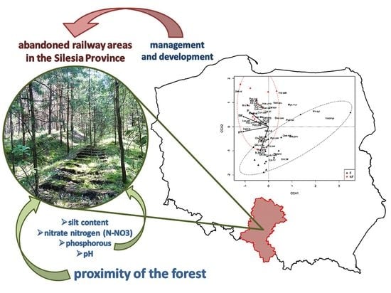
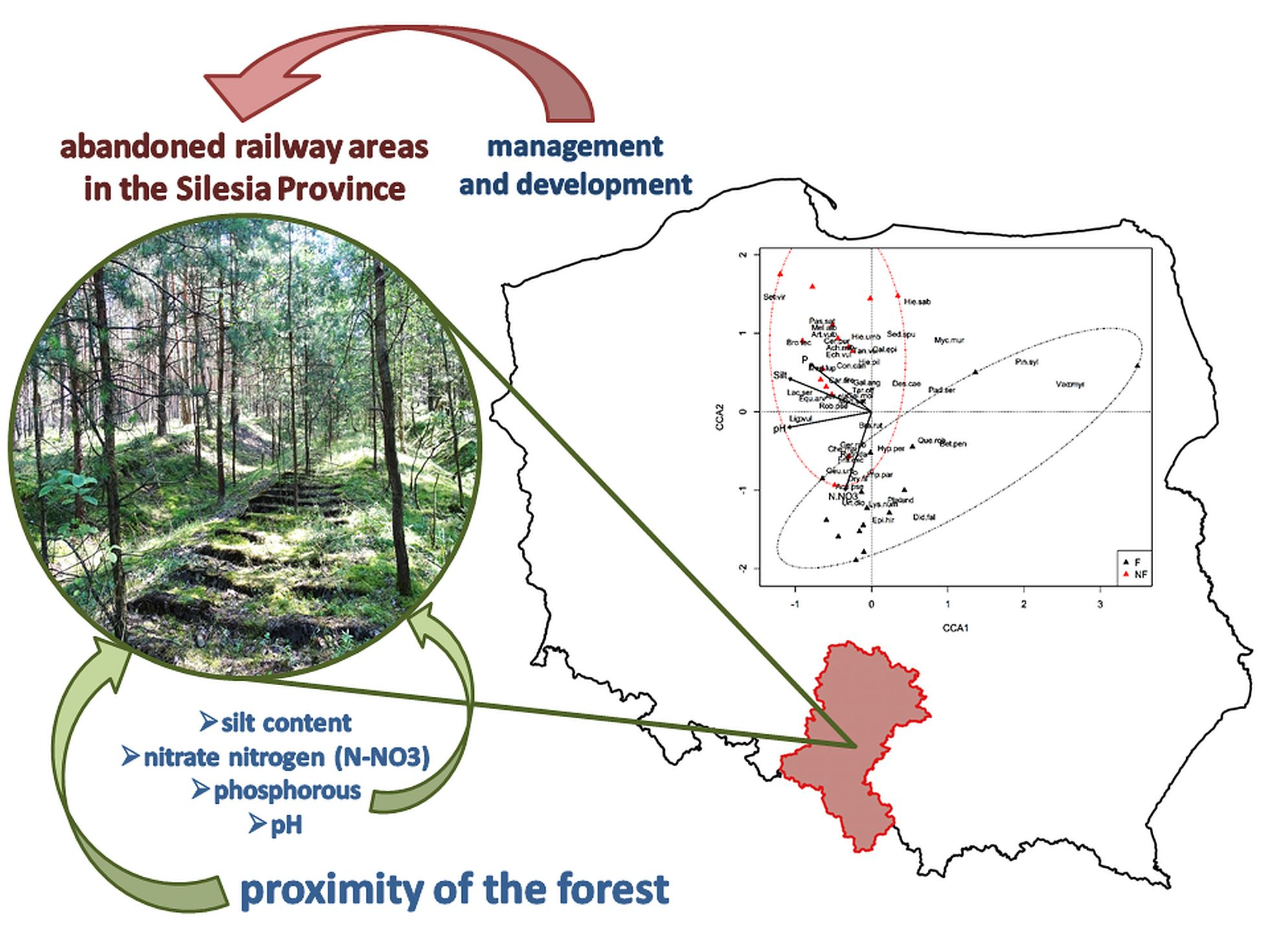
Factors Affecting Plant Composition in Abandoned Railway Areas with Particular Emphasis on Forest Proximity

Institute of Biology, Biotechnology and Environmental Protection, Faculty of Natural Sciences, University of Silesia in Katowice, 28 Jagiellońska Street, 40-032 Katowice, Poland
*
Author to whom correspondence should be addressed.
Diversity 2022, 14(12), 1141; https://doi.org/10.3390/d14121141
Submission received: 24 October 2022 / Revised: 14 December 2022 / Accepted: 16 December 2022 / Published: 19 December 2022
(This article belongs to the Special Issue Changes and Evolution of Flora and Vegetation under Human Impacts)

Abstract

:
Abandoned railway areas are places for the spontaneous spread of plants and the formation of specific plant communities. However, only limited information on this subject is available in the literature. The study aimed to determine the direction and the rate of forest formation, taking into account selected environmental factors. A floristic, phytosociological, and soil survey was carried out on a set of abandoned railway lines in the Silesia Province (southern Poland). For this purpose, 30 plots of vegetation were selected: 15 located in the vicinity of forests (F) and 15 surrounded by ruderal or segetal communities (NF). As a result, a total of 132 species (121 vascular plants and 11 mosses) were recorded, including 83 species at F plots and 78 species at NF plots. During the research, 13 syntaxa were distinguished. It was found that silt content, nitrate nitrogen (N-NO3), pH, and phosphorous have a significant impact upon which species dominated in the surveyed areas. It was found that the proximity of the forest was a crucial factor in determining the development of forest communities on abandoned railway areas. These results can be helpful for understanding how environmental conditions shape the forest structure on these types of habitats.

Graphical Abstract

1. Introduction

Human activity has a diverse impact on the natural environment, including the direction of succession [1]. This phenomenon has long been of interest to many researchers, e.g., [2,3,4,5,6,7,8,9,10,11,12,13,14], and the return of forest to secondary habitats has been the subject of numerous publications, e.g., [15,16,17,18,19,20,21,22,23,24,25,26]. This work is about plants growing on abandoned railway lines in southern Poland.
The 19th century was a period of rapid railway transport network expansion, with its most intensive development at the turn of the 19th and 20th centuries [27]. In these times, railway lines became an important element of the land transport infrastructure connecting cities and villages [28]. The first was opened in the United Kingdom in 1830. In Silesia, the first railway line was the Wrocław–Mysłowice route that led to the Upper Silesian Coal Basin and was opened in 1846 [29]. The heyday of railroad dominance has ended, however, and economic changes and the development of road transport in Poland after 1989 has resulted in the closure of many railway lines [30,31,32]. These have now turned into habitats spontaneously colonized by plant species encroaching from the immediate surroundings. Such effect has consequently led to the development of specific plant communities.
The closure of railway lines has been observed not only in Poland, but also in other European countries, and the outcome has been the same. The flora and vegetation of railway areas have been studied by many authors, e.g., [17,19,24,33,34,35,36,37,38,39,40]. However, most of these studies concern active railway lines or stations. Some researchers draw special attention to the so-called “railroad specialists”, i.e., plants occurring exclusively (or mostly) along railway lines [18,39,41,42]. The impact of functioning railway tracks on the vegetation of adjacent areas has been researched, e.g., [43,44]. Other publications concern the flora of railway embankments [45,46,47]. There is, however, a need to realize processes taking place in areas that are excluded from “railway use”.
Abandoned railway areas are a specific type of anthropogenic habitat where ecological succession towards forest communities may occur. Unfortunately, there are relatively few publications on the occurrence of plants in these types of habitats. Still, research aimed at determining changes in the flora structure of abandoned railway areas in Poland was conducted by Galera et al. [30] and Hutniczak et al. [48]. Indeed, a comparative analysis of the flora of three types of railway areas (active railway areas, railway areas abandoned less than 10 years ago, and railway areas abandoned more than 10 years ago) in north-eastern Poland can be found in the study by Galera et al. [49].
As evidenced by the research carried out in closed railway areas, ruderal flora often undergoes transformations towards synanthropic forest communities [17,18,19,20,24,25,30]. We therefore wanted to aim towards determining the factors affecting forest formation in abandoned railway areas. The objective of this study was to answer the following questions:
  • Which species dominate in the abandoned railway areas and what are their habitat preferences?
  • After what amount of time do forest communities develop in this type of habitat?
  • What environmental factors accelerate the rate of forest community formation?

2. Materials and Methods
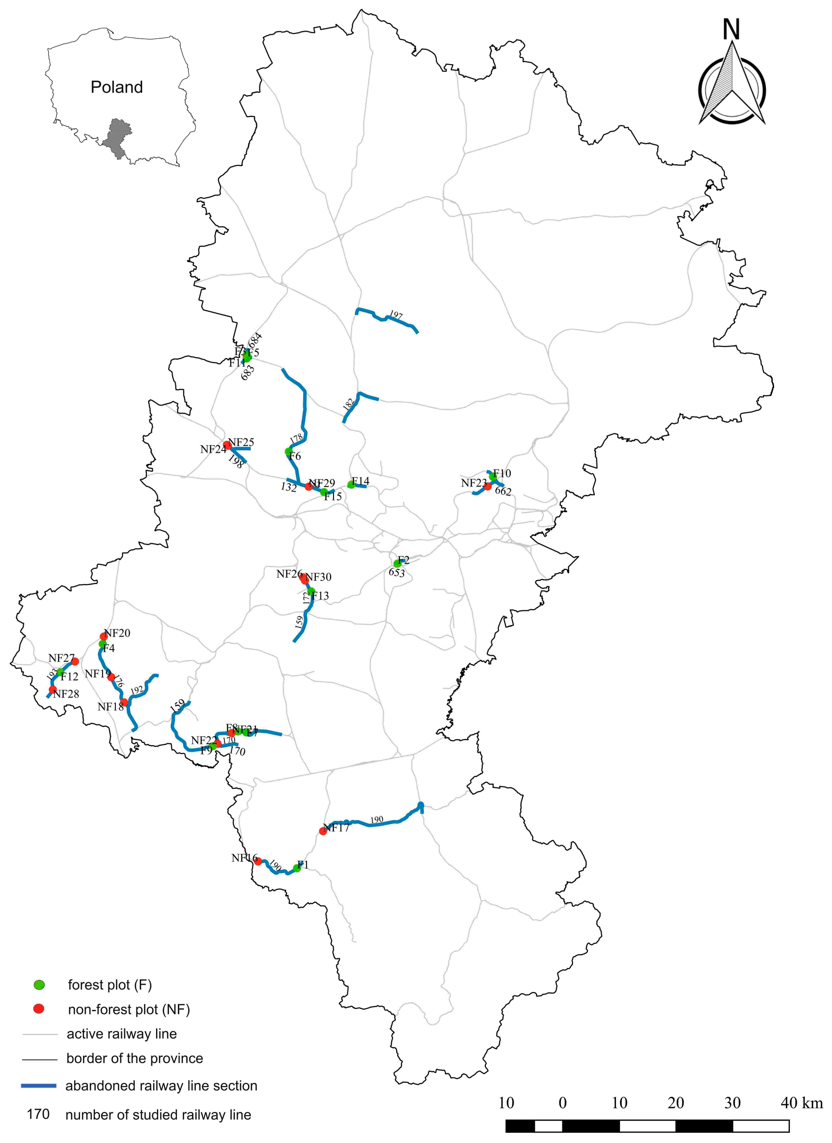
2.1. Study Area

The survey covered selected sections of abandoned railway lines in the Silesia Province (Figure 1), which is the most densely populated (366 persons/ km2) and industrialized area in Poland, covering 12,333 km2. The average yearly temperature (2001–2010) was 8.8 °C and the average annual precipitation sum was 770 mm [50].
The forest cover of the Silesia Province is 32.1%. Public forests account for 80.5% of the total forest land, while private forests account for 19.5%. The State Treasury owns 79.6% of the forest land, of which 97.8% is managed by the State Forests. The study area is dominated by lowland mixed coniferous and mixed forests. The most common forest-forming species are pine, oak, spruce, and birch [50].

2.2. The Field Research

The field research on the species composition of the flora (vascular plants and mosses) was carried out in 2016. A total of 30 sections of abandoned railway lines were selected, each with an area of 20 m2 and plant cover of at least 70% (Figure 1, Table 1). Fifteen sampling plots were located in the immediate vicinity of forests (F) and another 15 were surrounded by ruderal or segetal vegetation (NF). The number of the examined railway lines (e.g., railway line No. 190) and the year in which they were closed/excluded from “railway use” are given after Stankiewicz and Stiasny [51], as well as the National Railway Database [52]. The mean age of the plots was quite similar in the established groups (13.53 years in the F plots and 13.07 years in NF plots) (based on Stankiewicz and Stiasny [51], as well as the National Railway Database [52]). Phytosociological relevés were made at the study plots using the Braun-Blanquet method [53], taking into account the following vegetation layers: A, trees (>5 m high); B, shrubs (0.5–5 m); C, herbs (<0.5 m); D, mosses. The cover-abundance of species was assessed using the Braun-Blanquet scale, modified by Van Der Maarel [54]. Phytosociological relevés were taken at all the examined plots. Plant communities were distinguished based on diagnostic species [55]. The phytosociological relevé records in the tables were arranged considering the floristic similarity within the distinguished syntaxa. The nomenclature and systematics of vascular plant species were adopted after Mirek et al., [56] and mosses after Ochyra et al., [57]. The following aspects were defined for each species (except mosses): geographical and historical group [56,58], life form [59], phytosociological affinity [55,59], life strategy [60], and dispersal method [60]. The mean values for selected ecological indicators related to the light (L), temperature (T), and soil reaction (R) were calculated based on Ellenberg and Leuschner [61].

2.3. Soil Analysis

In August 2016, soil samples were collected from all of the sampling plots at a depth of 0–30 cm using a soil sampler and an auxiliary spatula. Each bulk sample consisted of 5 small subsamples mixed together. Before the laboratory analyses, the samples were dried, sieved through 2 mm mesh, and cleaned of any plant residues. The detailed methodology for soil parameters is presented in Table 2. Soil analyses were performed by the accredited Centre for Environmental Testing and Control in Katowice.
The soil texture was analyzed by Casagrande by applying the Prószyński modification areometric method, and the division into soil particle size fractions was established according to USDA standards [62]. As per this classification, soil and mineral formations were divided into groups and subgroups by weight percentage of sand, silt, and clay fraction in the earthy parts.

2.4. Data Analysis

All statistical analyses were conducted using R 3.5.2 version software [63].
Before conducting the analyses, the soil data were square root transformed to remove some of the skewness. In contrast, the plant species data were not transformed as they contained a high number of 0 values.
The parameters related to the soil and species traits were compared using a Mann–Whitney U test with significance level established at p ≤ 0.05. The Shannon–Wiener diversity index (H′) was calculated based on the formula:
H = i = 1 S p i l n p i
where S is the number of species, pi is the proportion of total sample represented by species i, and ln is the natural log.
In order to identify the general pattern of variation in the species composition of the F and NF plots, an indirect ordination method in the form of detrended correspondence analysis (DCA) was applied to the species data. The mean Ellenberg indicator values (EIV) for light (L), temperature (T), and soil reaction (R) were firstly tested using the Monte Carlo approach with 999 permutations and then the significant indicators were displayed on the DCA plot (R 3.5.2 version software [63]).
Species response curves based on the general linear models (GLM) were created subsequently in order to identify the main shifts in the species composition on both F and NF plots in relation to the gradient, which is presented by the time after the railway was closed (R 3.5.2 version software [63]).
To discover the relationship between soil factors and species distribution on the selected plots, the canonical correspondence analysis (CCA) was employed on species data with plant species that had at least 10% frequency or had high abundance (65 species) on the plots. The physicochemical soil properties were first assessed for co-linearity using variance inflation factor (VIF) testing. The variables related to the dry weight, humus level, total organic carbon, content of zinc, calcium, and sand were removed from the initial model as they all had VIF > 10. The most significant factors were obtained from the reduced model via forward selection procedure with 9999 permutations.

2.5. Abbreviations: The following Abbreviations Have Been Used in this Paper

  • Life strategy: C—competitor, S—stress tolerator, R—ruderal, CR—competitive ruderal, CS—stress tolerant competitor, SR—stress tolerant ruderal, CSR—intermediate;
  • Selected ecological indicators: L—light, T—temperature, R—soil reaction;
  • Species names: Ace.pla—Acer platanoides, Ace.pse—Acer pseudoplatanus, Ach.mil—Achillea millefolium, Aeg.pod—Aegopodium podagraria, Arr.ela—Arrhenatherum elatius, Art.vul—Artemisia vulgaris, Bet.pen—Betula pendula, Bra.rut—Brachythecium rutabulum, Bra.sal—Brachythecium salebrosum, Bro.tec—Bromus tectorum, Bry.cae—Bryum caespiticium, Cal.epi—Calamagrostis epigejos, Cal.sep—Calystegia sepium, Car.are—Cardaminopsis arenosa, Cer.hol—Cerastium holosteoides, Cer.pur—Ceratodon purpureus, Che.maj—Chelidonium majus, Con.arv—Convolvulus arvensis, Con.can—Conyza canadensis, Dau.car—Daucus carota, Des.ces—Deschampsia caespitosa, Did.fal—Didymodon fallax, Dry.car—Dryopteris carthusiana, Dry.fil—Dryopteris filix—mas, Ech.cru—Echinochloa crus—galli, Ech.vul—Echium vulgare, Epi.hel—Epipactis helleborine, Epi.hir—Epilobium hirsutum, Equ.arv—Equisetum arvense, Equ.syl—Equisetum sylvaticum, Eri.ann—Erigeron annuus, Eup.can—Eupatorium cannabinum, Fra.aln—Frangula alnus, Fra.exc—Fraxinus excelsior, Gal.ang—Galeopsis angustifolia, Gal.mol—Galium mollugo, Ger.rob—Geranium robertianum, Geu.urb—Geum urbanum, Hie.pil—Hieracium pilosella, Hie.sab—Hieracium sabaudum, Hie.umb—Hieracium umbellatum, Hyp.per—Hypericum perforatum, Imp.par—Impatiens parviflora, Lac.ser—Lactuca serriola, Lam.mac—Lamium maculatum, Lat.syl—Lathyrus sylvestris, Lig.vul—Ligustrum vulgare, Lin.vul—Linaria vulgaris, Lot.cor—Lotus corniculatus, Lys.num—Lysimachia nummularia, Med.lup—Medicago lupulina, Med.sat—Medicago sativa, Mel.alb—Melilotus alba, Myc.mur—Mycelis muralis, Oen.bie—Oenothera biennis, Pad.ser—Padus serotina, Pas.sat—Pastinaca sativa, Pim.sax—Pimpinella saxifraga, Pin.syl—Pinus sylvestris, Pla.lan—Plantago lanceolata, Pla.maj—Plantago major, Pla.und—Plagiomnium undulatum, Poa.ann—Poa annua, Poa.com—Poa compressa, Poa.pra—Poa pratensis, Que.rob—Quercus robur, Res.lut—Reseda lutea, Rob.ps—Robina pseudoacacia, Rub.cae—Rubus caesius, Rub.ida—Rubus idaeus, Rub.pli—Rubus plicatus, Rub.wim—Rubus wimmerianus, Rum.ace—Rumex acetosa, Sam.nig—Sambucus nigra, Scl.ann—Scleranthus annuus, Sed.spu—Sedum spurium, Set.vir—Setaria viridis, Sil.vul—Silene vulgaris, Sol.can—Solidago canadensis, Sol.gig—Solidago gigantea, Ste.med—Stellaria media, Tan.vul—Tanacetum vulgare, Tar.off—Taraxacum officinale, Tor.jap—Torilis japonica, Tri.arv—Trifolium arvense, Urt.dio—Urtica dioica, Vac.myr—Vaccinium myrtillus, Ver.cha—Veronica chamaedrys, Vic.cra—Vicia cracca, Vio.rei—Viola reichenbachiana.

3. Results

3.1. Flora and Vegetation

In total, 121 species of vascular plants and 11 moss species were recorded at 30 plots, 83 species (including 10 mosses) at F plots, and 78 species (including 5 mosses) at NF plots. The number of species found at individual plots varied significantly (4–24).
The most frequent species at the plots adjacent to non-forest communities were: Arrhenatherum elatius, Convolvulus arvensis, Artemisia vulgaris, Rubus caesius, and Vicia cracca, whereas Geranium robertianum, Geum urbanum, Impatiens parviflora, Urtica dioica, and Rubus caesius were most common at the plots located in the vicinity of forests.
Larger differences between F and NF plots were observed when analyzing the cover of each vegetation layer (stratum). Layers A and B were not found at the plots adjacent to NF areas regardless of the year of their closure, whereas if a given plot was surrounded by forest communities, layer B developed already in the 2 years after closing and layer A after 21 years post-closure.
There was no clear distinction between F and NF plots in terms of species richness and diversity (Table 3). The percentage cover of the vegetation was slightly higher on the NF plots (94.67%) compared with the F plots (88%). The consequent result of the proximity to the forest areas was a higher cover of the shrub and tree layer on the F plots, though some of the plots in this category remained completely uncovered. Native species dominated in all the study plots. There were no statistically significant differences between F and NF plots in terms of geographical and historical groups, life forms (except for the number of phanerophytes and moss cover), or dispersion ways. It was found that species with CS (stress tolerant competitor) and SR (stress tolerant ruderal) strategies were more abundant at the plots located in the vicinity of forested areas, while species utilizing a CR (competitive ruderal) strategy dominated at the plots adjacent to non-forest vegetation.
Most of the species at the plots located in the vicinity of the forest areas belonged to the classes Artemisietea vulgaris (16 species) and Querco-Fagetea (13), while classes Artemisietea vulgaris (20), Molinio-Arrhenatheretea (17), and Stellarietea mediae (13 species) were most frequently represented at the plots located in the vicinity of non-forest vegetation. Species from the class Alnetea glutinosae and Vaccinio-Piceetea appeared at plots surrounded by forest areas only.
During the study, 13 syntaxa were distinguished, including 5 as associations and 8 as communities. They belonged to six phytosociological classes: Stellarietea mediae, Epilobietea angustifolii, Artemisietea vulgaris, Molinio-Arrhenatheretea, Vaccinio-Piceetea, and Querco-Fagetea. On the F plots, five communities (with Acer pseudoplatanus, Fraxinus excelsior, Pinus sylvestris, Urtica dioica, and Betula pendula-Populus tremula) and two associations (Impatientetum parviflorae and Epilobio-Geranietum robertiani) were described. The most frequent was the Impatientetum parviflorae association. Three communities (Galeopsis angustifolia, Rubus caesius, and Sedum spurium) and four associations (Arrhenatheretum elatioris, Corispermo-Brometum tectorum, Echio-Melilotetum, and Epilobio-Geranietum robertiani) were formed on NF plots (Arrhenatheretum elatioris was the most frequent syntaxon). One of the noted associations—Epilobio-Geranietum robertiani—appeared on both types of tested plots.

3.2. Soil Properties

Physicochemical results of the soil analyses (Table 4) indicate that, in terms of soil condition, the statistical differences between F and NF plots were related to the content of phosphorous and also the granulometric composition of the soil substrate. The soil on the NF plots was characterized by a higher content of P, a slightly higher content of both clay and silt fractions, and also a lower content of the sand fraction compared with the soil from the F plots.

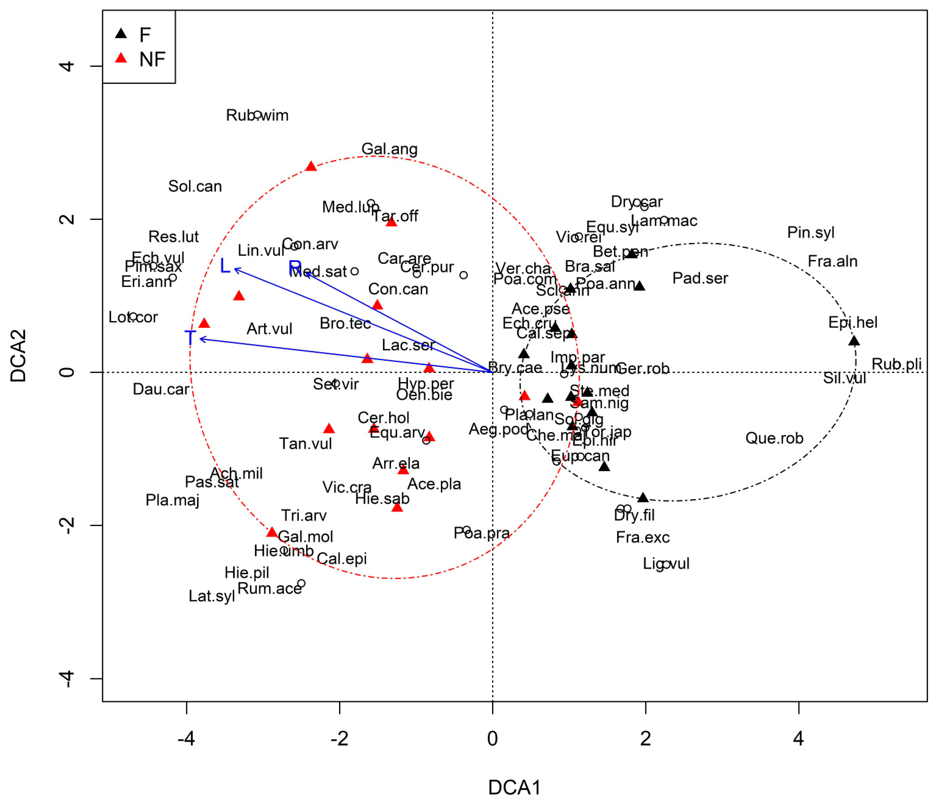
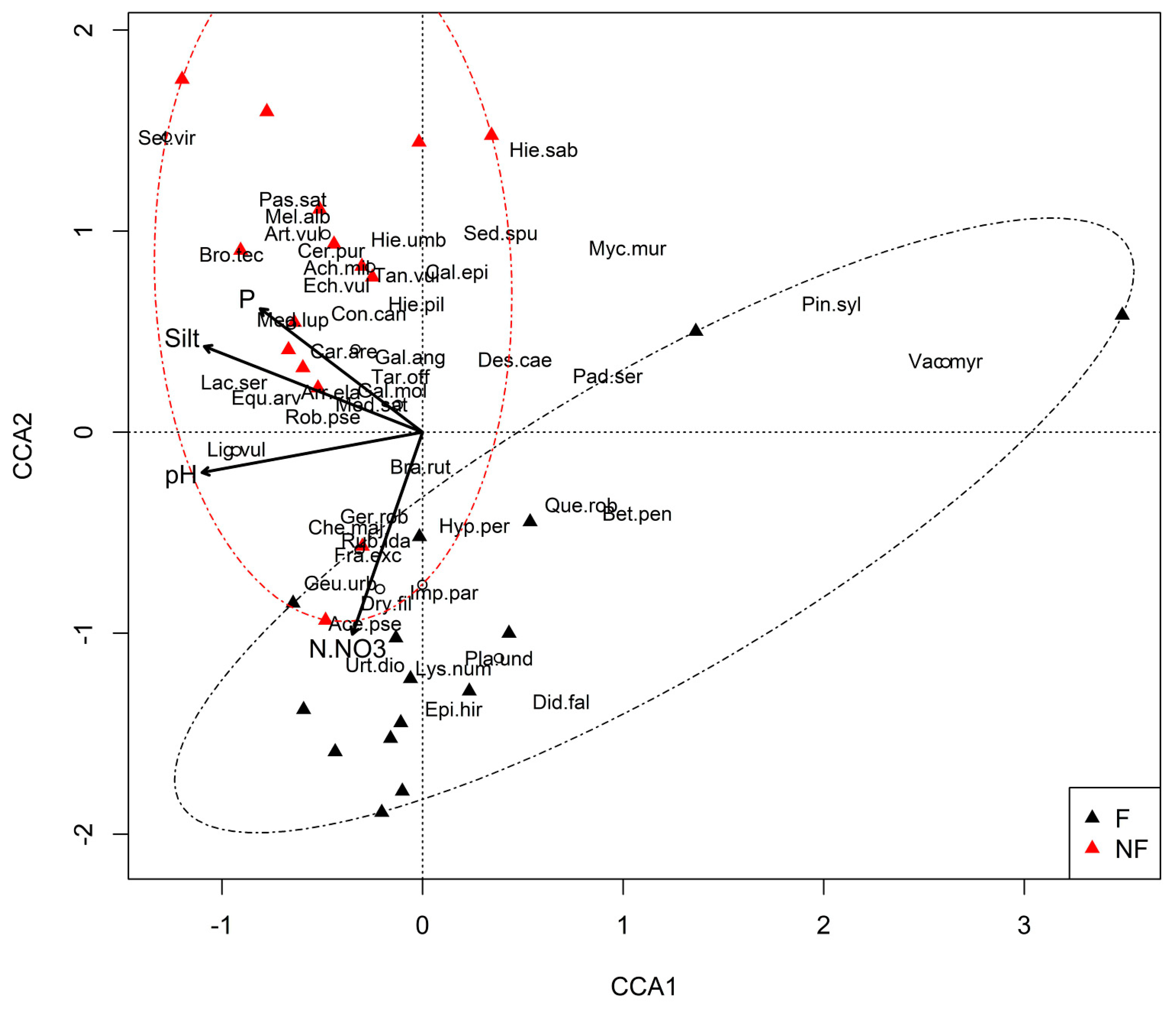
3.3. Plant Communities and Their Relationships with the Environmental Factors

Species variation across the plots was clearly noticeable with ecological gradients defined by the DCA axes (Figure 2). Two groups of species can be distinguished. The first is mainly associated with the F plots, comprising species that are commonly present in the forest communities, e.g., Dryopteris carthusiana, D. filix-mas, Epipactis helleborine, Equisetum sylvaticum, Eupatorium cannabinum, Frangula alnus, Fraxinus excelsior, Geranium robertianum, Lamium maculatum, Ligustrum vulgare, Padus serotina, Pinus sylvestris, Quercus robur, Viola reichenbachiana, and mosses (Brachythecium salebrosum, Bryum caespiticium). The second group is related to the NF plots and includes species found mainly on the slopes of railway embankments, wastelands, and near farmlands such as Convolvulus arvensis, Daucus carota, Echium vulgare, Erigeron annuus, Galeopsis angustifolia, Hypericum perforatum, Linaria vulgaris, Reseda lutea, or Solidago canadensis. In contrast to forest species, they are characterized by higher values of the ecological indicators of light (L), temperature (T), and soil reaction (R).
The probability of species occurrence along the gradient that is related to the time that passed after the railway was closed (Figure 3) indicates some substantial shifts in the species composition on the examined plots. In the first few years after abandonment, we noted that the plots were mainly covered by plant species with a high tolerance for light and which typically occupied meadows, ruderal habitats, and wastelands around the arable lands (Figure 3A). Over time, their occurrence decreased. At the same time, woody species and those that preferred less temperature and more shading occurred more frequently (Figure 3B).
The results of the conducted CCA analysis (Figure 4) indicate that the difference between F and NF plots is noticeable in terms of species–environment relations; although, some of the plots from both types were grouped together. The first axis accounted for 36.8% of the total variation in species composition and was mainly correlated with variables such as pH (r = −0.80), content of phosphorous (r = −0.59), and content of silt (r = −0.79). These factors mainly affected species diversity in the NF plots. The second axis accounted for 29.9% of the total variation in the species data and was correlated with the content of the nitrate nitrogen (r = −0.73), whose concentration was higher in the F plots.

4. Discussion

Most of the species occurring on abandoned railway lines are characteristic of the class Artemisietea vulgaris due to their adaptation to both ruderal and forest–thicket habitats. These are often native large nitrophilous perennials that tolerate shade and quickly colonize a given area, preventing other species from developing there. On the examined surfaces there were: Artemisia vulgaris, Convolvulus arvensis, Geranium robertianum, Geum urbanum, Rubus caesius, and Urtica dioica. Many of these species are also mentioned as frequent by other authors [17,30,34,49,64,65]. However, these data relate mainly to active railway lines.
Due to the fact that track ground conditions differ from the surroundings, the encroachment of species from the vicinity is limited; this especially concerns species that are particularly sensitive to human activities. The rate of forest regeneration depends mainly on the availability of species diaspores that prefer this type of vegetation. When the railway line is closed, there is a possibility of creating a forest on its territory. Authors who have compared the flora of active and abandoned railway lines after their exclusion from use have observed a decrease in the number of species of foreign origin with a short life cycle (therophytes) and then the appearance of perennial native species. These changes took place very quickly, just a few years after closing lines [19,24,30,49,66,67]. It is interesting to note that, in the stages of succession in this type of habitat, the forest arises “from the top”; layers B and A are formed firstly and then C [25].
In the study area, the most common forest species were: Acer platanoides, A. pseudoplatanus, Betula pendula, Fraxinus excelsior, and Pinus sylvestris. Similar species dominated in the railway areas of north-eastern Poland [25] and Lower Saxony [17].
Seedlings and young specimens of trees and shrubs are also found on operating railway lines [25]. Due to human activity, however, they are not able to reach larger sizes. The succession towards forest communities is possible only when railway lines are taken out of service [30]. The arrival of species characteristic of this type of vegetation is, however, hampered by a number of factors. One of these may be the lack of shade and the related low moisture content in the soil (which is connected with the absence of shrubs and trees). Based on the obtained results, it was found that layers A and B appeared only on plots adjacent to forest areas after 21 and 2 years, respectively. In a related study [30], we can find information that on closed railway lines located near the forest, layer A developed the soonest after 14 years. In the case of surroundings being non-forest communities (grasslands), layer A did not appear (railway lines with a maximum of 16 years’ closure were tested), while layer B on one of the plots occurred after 9 years. Hence, if there are no forests in the nearby vicinity, the development of forest does not seem possible in less than a few dozen years. The situation is different when railway areas are located in the vicinity of forested areas. In such a case, the process of succession may be much faster, e.g., the shrub layer may develop after just a few years and trees become established after several years. This has also been confirmed by the current research. According to Taylor [27], “Typically, a railway line left in the field becomes overgrown with grass and shrubs and, if it runs through forested areas, also by trees”. Murray et al. [68] point out that species composition of the flora in this type of habitat is affected not only by light or moisture conditions, but also by the type of vegetation occurring in the vicinity of railway tracks. The proximity of forest areas, and thus the supply of diaspores of phanerophytes and chamaephytes in the early stages of succession, is, therefore, a very important precondition for the accelerated rate of change towards forest communities.
It has been found that life strategies C, CSR, and CR are represented by the largest number of species in the study plots. Similar results were obtained by Wrzesień et al., [28], who studied railway areas in Lublin and Lviv. Statistically significant differences between the studied areas were noted for species with a CS or SR strategy (more numerous on F plots) and a CR strategy (characteristic for NF plots).
Galera et al. [30] reported a decline in the number of anemochorous species in relation to the zoochorous species along with the time that elapsed since the railway line was closed. Our research has not confirmed this relationship clearly. However, when comparing F with NF plots, it has been found that the relative abundance of zoochores at the former sites is about 10% higher.
Most soil parameters on the studied surfaces did not have a significant impact on the species composition and their values did not show a large variation. Similar results were obtained by other authors [19,25,69].
The type of plant communities occurring in the vicinity of the surveyed sites is of key importance. If these are forest communities, the course of succession may follow one of two paths depending on soil properties. In the case of low pH and sandy soils with a low content of nitrogen, coniferous forest species begin to occur and the tree layer is dominated by pine, oak, and birch. On soils rich in nitrogen, with a higher content of loam fractions and a higher reaction, succession leads to the development of forest communities of a synanthropic nature, with a significant contribution of sycamore, maple, and ash. In areas surrounded by non-forest communities, succession has a different course. Due to the lack of the direct inflow of diaspores, it is very difficult for forest species to arrive at this type of habitat and probably this can happen only after a much longer time. Instead of forest, synanthropic communities develop, dominated by plants from the class Artemisietea vulgaris and Molinio-Arrhenatheretea. To determine the subsequent stages of succession in this type of areas, further research is needed that will allow for a longer period of time (at least dozens of years) since the railway lines’ closures.
It should be emphasized that understanding the plant biodiversity on railway tracks is vitally important for future perspectives and management of these areas [70].

5. Conclusions

  • The type of plant communities occurring in the immediate vicinity of the abandoned railway lines has a major impact on which species dominate in the developing communities. In the vicinity of forests, these are acidophilous, CS and SR strategies, zoochorous, and shade-tolerant species, whereas basiphilous, CR strategies, anemochorous, heliophilous, and species that prefer loamy soils dominate when a given area is surrounded by non-forest communities.
  • The proximity of forested areas determinates a higher rate of succession towards forest communities. A similar role is played by grain-size composition of the soil; the process is faster on sandy soils. Other soil parameters (except pH, nitrate nitrogen, and phosphorous content) are of relatively minor importance.
  • Forest communities may develop on abandoned railway areas after several years provided there are forests growing in their vicinity. However, these are synanthropic communities whose herb layer significantly deviates from typical forests.
  • The obtained results can be used by various institutions dealing with managing and developing of such areas to revitalize them.

Author Contributions

Conceptualization, A.U. (Alina Urbisz) and A.U. (Andrzej Urbisz); methodology, A.H., A.U. (Alina Urbisz), and A.U. (Andrzej Urbisz); software, A.U. (Andrzej Urbisz) and Ł.S.; validation, A.H. and A.U. (Alina Urbisz); formal analysis, A.U. (Andrzej Urbisz) and Ł.S.; investigation, A.H. and A.U. (Alina Urbisz); resources, A.H., A.U. (Alina Urbisz), and A.U. (Andrzej Urbisz); data curation, A.H.; writing—original draft preparation, A.H., A.U. (Alina Urbisz), and A.U. (Andrzej Urbisz); writing—review and editing, A.H., A.U. (Alina Urbisz), A.U. (Andrzej Urbisz), and Ł.S.; visualization, A.U. (Andrzej Urbisz) and Ł.S.; supervision, A.U. (Alina Urbisz); project administration, A.U. (Alina Urbisz); funding acquisition, A.U. (Alina Urbisz). All authors have read and agreed to the published version of the manuscript.

Funding

The research was partially financed from the funds for statutory activities Faculty of Biology and Environmental Protection of the University of Silesia in Katowice for the development of young scientists research project for doctoral students (project title: “The species composition of the flora of the abandoned railway areas of Silesia Province depending on the selected soil parameters”).

Institutional Review Board Statement

Not applicable.

Data Availability Statement

Not applicable.

Acknowledgments

The authors would like to thank Barbara Fojcik for her assistance with the identification of bryophytes and Krzysztof Oklejewicz for the verification of specimens from the genus Rubus. In addition, the authors would like to sincerely thank Iwona Steczek for her help in preparing Figure 1. The authors are also grateful to employees of the PKP Management Board for providing the unpublished information on railway areas. Moreover, the authors would like to thank a native speaker for language support and corrections. We are thankful to Michael Wink and Bogdan Jackowiak for organizing this issue and inviting us to contribute.

Conflicts of Interest

The authors declare no conflict of interest.

References

  1. Faliński, J.B. Sukcesja roślinności na nieużytkach porolnych jako przejaw dynamiki ekosystemu wyzwolonego spod długotrwałej presji antropogenicznej [The succession of vegetation on agricultural wastelands as a manifestation of the dynamics of the ecosystem liberated from long-term anthropogenic pressure]. Wiadomości Bot. 1986, 30, 25–50. (In Polish) [Google Scholar]
  2. Clements, F.E. Plant Succession: An Analysis of the Development of Vegetation; Carnegie Institution of Washington: Washington, DC, USA, 1916; pp. 1–512. [Google Scholar]
  3. Clements, F.E. Plant Succession and Indicators: A Definitive Edition of Plant Succession and Plant Indicators; The H.W. Wilson Company: New York, NY, USA, 1928; pp. 1–453. [Google Scholar]
  4. Gleason, H.A. The individualistic concept of the plant association. Am. Midl. Nat. 1939, 21, 92–110. [Google Scholar] [CrossRef]
  5. Bazzaz, F.A. Succession on abandoned fields in the Shawnee Hills, Southern Illinois. Ecology 1968, 49, 924–936. [Google Scholar] [CrossRef]
  6. Horn, H.S. The ecology of secondary succession. Annu. Rev. Ecol. Evol. Syst. 1974, 5, 25–37. [Google Scholar] [CrossRef]
  7. Finegan, B. Forest succession. Nature 1984, 312, 109–114. [Google Scholar] [CrossRef]
  8. Pickett, S.T.A.; Collins, S.L.; Armesto, J.J. A hierarchical consideration of causes and mechanisms of succession. Vegetatio 1987, 69, 109–114. [Google Scholar] [CrossRef]
  9. Pickett, S.T.A.; Collins, S.L.; Armesto, J.J. Models, Mechanisms and Pathways of Succession. Bot. Rev. 1987, 53, 335–371. [Google Scholar] [CrossRef]
  10. Glenn-Lewin, D.C.; Peet, R.K.; Veblen, T.T. (Eds.) Plant Succession. Theory and Prediction; Chapman & Hall: London, UK; New York, NY, USA, 1992; pp. 1–352. [Google Scholar]
  11. Botkin, D.B. Forest Dynamics—An Ecological Model; Oxford University Press: Oxford, UK, 1993; pp. 1–309. [Google Scholar]
  12. Wiegleb, G.; Felinks, B. Primary succession in post-mining landscapes of Lower Lusatia—Chance or necessity. Ecol. Eng. 2001, 17, 199–217. [Google Scholar] [CrossRef]
  13. Zipperer, W.C. The process of natural succession in urban areas. In The Routledge Handbook of Urban Ecology; Douglas, I., Goode, D., Houck, M., Wang, R., Eds.; Routledge Press: London, UK, 2011; pp. 187–197. [Google Scholar]
  14. Chang, C.C.; Turner, B.L. Ecological succession in a changing world. J. Ecol. 2019, 107, 503–509. [Google Scholar] [CrossRef] [Green Version]
  15. Shantz, H.L. Plant Succession on Abandoned Roads in Eastern Colorado. J. Ecol. 1917, 5, 19–42. [Google Scholar] [CrossRef] [Green Version]
  16. Roux, E.R.; Warren, M. Plant Succession on abandoned fields in central Oklahoma and in the Transvaal Highveld. Ecology 1963, 44, 576–579. [Google Scholar] [CrossRef]
  17. Brandes, D. Flora und Vegetation der Bahnhöfe Mitteleuropas. Phytocoenologia 1983, 11, 31–115. [Google Scholar] [CrossRef]
  18. Brandes, D. Eisenbahnanlagen als Untersuchungsgegenstand der Geobotanik. Tuexenia 1993, 13, 415–444. [Google Scholar]
  19. Kowarik, I.; Tietz, B. Soils on ruined railway stations—The Anhalter Güterbahnhof. In XIII Congress of the International Society of Soil Science (Hamburg, Germany)—Guidebook Tours G and H: Soilscapes of Berlin (West): Natural and Anthropogenic Soils and Environmental Problems within a Metropolitan Area; Alaily, F., Grenzius, R., Renger, M., Stahr, K., Tietz, B., Wessolek, G., Eds.; Mitteilungen Deutsche Hamburg, Germany Bodenkundliche Gesellschaft 50; 1986; pp. 128–139. [Google Scholar]
  20. Kowarik, I.; Langer, A. Vegetation einer Berliner Eisenbahnfläche (Schöneberger Südgelände) im vierten Jahrzehnt der Sukzession. Verh. Der Bot. Ver. Berl. Brandenbg. 1994, 127, 5–43. [Google Scholar]
  21. Prach, K.; Pyšek, P.; Šmilauer, P. Prediction of vegetation succession in human disturbed habitats using an expert system. Restor. Ecol. 1999, 7, 15–23. [Google Scholar] [CrossRef] [Green Version]
  22. Prach, K.; Pyšek, P.; Bastl, M. Spontaneous vegetation succession in human-disturbed habitats: A pattern across seres. Appl. Veg. Sci. 2001, 4, 83–88. [Google Scholar] [CrossRef]
  23. Prach, K.; Lencová, K.; Řehounková, K.; Dvořáková, H.; Jírová, A.; Konvalinková, P.; Mudrák, O.; Novák, J.; Trnková, R. Spontaneous vegetation succession at different central European mining sites: A comparison across seres. Environ. Sci. Pollut. Res. 2013, 20, 7680–7685. [Google Scholar] [CrossRef]
  24. Schinninger, I.; Maier, R.; Punz, W. Der stillgelegte Frachtenbahnhof Wien-Nord Standortbedingungen und ökologische Charakteristik der Gefäßpflanzen einer Bahnbrache. Verh. Der Zool. Bot. Ges. Osterr. 2002, 139, 1–10. [Google Scholar]
  25. Galera, H.; Sudnik-Wójcikowska, B.; Wierzbicka, M.; Wiłkomirski, B. Encroachment of forest species into operating and abandoned railway areas in north-eastern Poland. Plant Biosyst. 2011, 145, 23–36. [Google Scholar] [CrossRef]
  26. Oikonomakis, N.; Ganatsas, P. Land cover changes and forest succession trends in a site of Natura 2000 network (Elatia forest), in northern Greece. Forest Ecol. Manag. 2012, 285, 153–163. [Google Scholar] [CrossRef]
  27. Taylor, Z. Rozwój i Regres Sieci Kolejowej w Polsce [The Growth and Contraction of the Railway Network in Poland]; Polish Academy of Sciences: Warsaw, Poland; Stanisław Leszczycki Institute of Geography and Spatial Organization: Warsaw, Poland, 2007; Monographies 7; pp. 1–322. (In Polish) [Google Scholar]
  28. Wrzesień, M.; Denisow, B.; Mamchur, Z.; Chuba, M.; Resler, I. Composition and structure of the flora in intra-urban railway areas. Acta Agrobot. 2016, 69, 1–14. [Google Scholar] [CrossRef]
  29. Dulias, R.; Hibszer, A. Województwo Śląskie—Przyroda, Gospodarka, Dziedzictwo Kulturowe [Silesian Voivodeship—Nature, Economy, Cultural Heritage]; Wydawnictwo Kubajak: Krzeszowice, Poland, 2004; pp. 9, 41–43, 141–142. (In Polish) [Google Scholar]
  30. Galera, H.; Sudnik-Wójcikowska, B.; Wierzbicka, M.; Wiłkomirski, B. Directions of changes in the flora structure in the abandoned railway areas. Ecol. Quest. 2012, 16, 29–39. [Google Scholar]
  31. Piskorz, R.; Czarna, A. Vascular plants on active and closed railway stations in Wolsztyn and its surroundings. Rocz. Akad. Rol. Pozn. Bot. Stec. 2006, 10, 137–156. [Google Scholar]
  32. Wrzesień, M.; Święs, F. Flora i Zbiorowiska Roślinne Terenów Kolejowych Zachodniej Części Wyżyny Lubelskiej [Flora and Vascular Plants Communities of Railway Areas of the Western Part of the Lublin Upland]; Wydawnictwo UMCS: Lublin, Poland, 2006; pp. 1–255. (In Polish) [Google Scholar]
  33. Niemi, Å. On the railway vegetation and flora between Esbo and lngå, S. Finland. Acta Bot. Fenn. 1969, 83, 1–28. [Google Scholar]
  34. Sargent, C. Britain’s Railway Vegetation; Institute of Terrestrial Ecology: Cambridge, UK, 1984; pp. 1–34. [Google Scholar]
  35. Jehlík, V. The Vegetation of Railways in Northern Bohemia (Eastern Part); Academia Publishing House of the Czechoslovak: Prague, Czech Republic; Academy of Sciences: Prague, Czech Republic, 1986; Vegetace ČSSR, ser. A, 14; pp. 1–366. [Google Scholar]
  36. Jandová, L.; Sklenář, P.; Kovář, P. Changes of Grassland Vegetation in Surroundings of New Railway Flyover (Eastern Bohemia, Czech Republic). Part I: Plant Communities and Permanent Habitat Plots. J. Landsc. Ecol. 2009, 2, 35–56. [Google Scholar] [CrossRef] [Green Version]
  37. Májeková, J.; Letz, D.R.; Slezák, M.; Zaliberová, M.; Hrivnák, R. Rare and threatened vascular plants of the railways in Slovakia. Biodivers. Res. Conserv. 2014, 35, 75–85. [Google Scholar] [CrossRef] [Green Version]
  38. Májeková, J.; Zaliberová, M.; Andrik, E.J.; Protopopova, V.V.; Shevera, M.V.; Ikhardt, P. A comparison of the flora of the Chop (Ukraine) and Čierna nad Tisou (Slovakia) border railway stations. Biologia 2020, 76, 1969–1989. [Google Scholar] [CrossRef]
  39. Altay, V.; Ozyigit, I.I.; Osma, E.; Bakir, Y.; Demir, G.; Severoglu, Z.; Yarci, C. Environmental relationships of the vascular flora alongside the railway tracks between Haydarpaşa and Gebze (Istanbul-Kocaeli/ Turkey). J. Environ. Biol. 2015, 36, 153–162. [Google Scholar] [PubMed]
  40. Denisow, B.; Wrzesień, M.; Mamchur, Z.; Chuba, M. Invasive flora within urban railway areas: A case study from Lublin (Poland) and Lviv (Ukraine). Acta Agrobot. 2017, 70, 1727. [Google Scholar] [CrossRef]
  41. Kornaś, J.; Leśniowska, I.; Skrzywanek, A. Observations on the flora of railway areas and freight stations in Cracow. Fragm. Florist. Geobot. Pol. 1959, 5, 199–216. [Google Scholar]
  42. Wierzbicka, M.; Galera, H.; Sudnik-Wójcikowska, B.; Wiłkomirski, B. Geranium robertianum L., plant form adapted to the specific conditions along railway: ”Railway-wandering plant”. Plant Syst. Evol. 2014, 300, 973–985. [Google Scholar] [CrossRef] [Green Version]
  43. Chen, H.; Li, S.; Zhang, Y. Impact of road construction on vegetation alongside Quinghai-Xizang highway and railway. Chinese Geogr. Sci. 2003, 13, 340–346. [Google Scholar] [CrossRef]
  44. Tikka, P.M.; Högmander, H.; Koski, P.S. Road and railway verges serve as dispersal corridors for grassland plants. Landsc. Ecol. 2001, 16, 659–666. [Google Scholar] [CrossRef]
  45. Fornal-Pieniak, B.; Wysocki, C. Flora nasypu nieużytkowanej linii kolejowej w okolicach Sokołowa Podlaskiego [Flora of a non-used railway embankment near Sokołów Podlaski]. Woda Sr. Obsz. Wiej. 2010, 10, 85–94. (In Polish) [Google Scholar]
  46. Kryszak, A.; Kryszak, J.; Czemko, M.; Kalbarczyk, M. Vegetation of embankment along selected railway lines. Zesz. Nauk. Uniw. Przyr. We Wrocławiu. Rol. 2006, 88, 159–164. (In Polish) [Google Scholar]
  47. Suominen, J. The plant cover of Finnish railway embankments and the ecology of their species. Ann. Bot. Fenn. 1969, 6, 183–235. [Google Scholar]
  48. Hutniczak, A.; Urbisz, A.; Wilczek, Z. Flora i Roślinność Nieużytkowanych Terenów Kolejowych Województwa Śląskiego [Flora and Vegetation of Abandoned Railway Areas of the Silesian Province]; Monographs of the Upper Silesian Museum 15; Muzeum Górnośląskie: Bytom, Poland, 2020; pp. 1–130. (In Polish) [Google Scholar]
  49. Galera, H.; Sudnik-Wójcikowska, B.; Wierzbicka, M.; Jarzyna, I.; Wiłkomirski, B. Structure of the flora of railway areas under various kinds of anthropopression. Pol. Bot. J. 2014, 59, 121–130. [Google Scholar] [CrossRef] [Green Version]
  50. Statistical Yearbook of Śląskie Voivodship. 2020. Available online: https://katowice.stat.gov.pl/download/gfx/katowice/en/defaultaktualnosci/665/1/20/1/rocznik_2020_internet_wersja_angielska.pdf (accessed on 23 October 2022).
  51. Stankiewicz, R.; Stiasny, M. Atlas Linii Kolejowych Polski 2014 [Atlas of Polish Railway Lines 2014]; Eurosprinter Publisher: Rybnik, Poland, 2014; pp. 1–464. (In Polish) [Google Scholar]
  52. Ogólnopolska Baza Kolejowa [National Railway Database]. Available online: https://www.bazakolejowa.pl/ (accessed on 20 June 2020).
  53. Braun-Blanquet, J. Pflanzensoziologie, Grundzüge der Vegetationskunde, 3rd ed.; (Phytosociology, the Basis of Vegetation Science); Springer: Wien, Austria; New York, NY, USA, 1964; Volume 3, pp. 1–865. [Google Scholar]
  54. Van Der Maarel, E. Transformation of Cover-Abundance Values in Phytosociology and Its Effects on Community Similarity. Vegetatio 1979, 39, 97–114. [Google Scholar]
  55. Matuszkiewicz, W. Przewodnik do Oznaczania Zbiorowisk Roślinnych Polski [Guide to the Determination of Polish Plant Communities]; PWN: Warsaw, Poland, 2017; pp. 1–536. (In Polish) [Google Scholar]
  56. Mirek, Z.; Piękoś-Mirkowa, H.; Zając, A.; Zając, M. Vascular Plants of Poland. An Annotated Checklist; W. Szafer Institute of Botany: Krakow, Poland; Polish Academy of Sciences: Cracow, Poland, 2020; pp. 1–442. [Google Scholar]
  57. Ochyra, R.; Żarnowiec, J.; Bednarek-Ochyra, H. Census Catalogue of Polish Mosses; Institute of Botany: Kraków, Poland; Polish Academy of Sciences: Cracow, Poland, 2003; pp. 1–372. [Google Scholar]
  58. Tokarska-Guzik, B.; Dajdok, Z.; Zając, M.; Zając, A.; Urbisz, A.; Danielewicz, W.; Hołdyński, C. Rośliny Obcego Pochodzenia w Polsce ze Szczególnym Uwzględnieniem Gatunków Inwazyjnych [Plants of Foreign Origin in Poland, with Particular Emphasis on Invasive Species]; Generalna Dyrekcja Ochrony Środowiska: Warsaw, Poland, 2012; pp. 1–196. (In Polish) [Google Scholar]
  59. Zarzycki, K.; Trzcińska-Tacik, H.; Różański, W.; Szeląg, Z.; Wołek, J.; Korzeniak, U. Ecological Indicator Values of Vascular Plants of Poland; W. Szafer Institute of Botany: Kraków, Poland; Polish Academy of Sciences: Cracow, Poland, 2002; pp. 1–183. [Google Scholar]
  60. Frank, D.; Klotz, S. Biologisch-Ökologische Daten zur Flora der DDR, 2nd ed.; Martin Luther Universität Halle—Wittenberg Wissenschaftliche Beiträge: Halle, Germany, 1990; pp. 33–160. [Google Scholar]
  61. Ellenberg, H.; Leuschner, C. Zeigerwerte der Pflanzen Mitteleuropas. In Vegetation Mitteleuropas mit den Alpen, 6th ed.; Verlag Eugen Ulmer: Stuttgart, Germany, 2010; pp. 1–66. [Google Scholar]
  62. Ryżak, M.; Bartmiński, P.; Bieganowski, A. Metody wyznaczania rozkładu granulometrycznego gleb mineralnych [Methods for determining the granulometric distribution of mineral soils]. Acta Agrophysica Rozpr. I Monogr. 2009, 4, 1–84. (In Polish) [Google Scholar]
  63. R Core Team 2019. R: A Language and Environment for Statistical Computing. R Foundation for Statistical Computing. Vienna. Austria. Available online: https://www.R-project.org/ (accessed on 12 November 2019).
  64. Messenger, K.G. A railway flora of Rutland. Proc. Bot. Soc. Br. Isl. 1968, 7, 325–344. [Google Scholar]
  65. Sudnik-Wójcikowska, B.; Galera, H.; Suska-Malawska, M.; Staszewski, T.; Wiłkomirski, B. Specyfika grupy najpospolitszych gatunków we florze silnie skażonych odcinków torowisk kolejowych w północno-wschodniej Polsce (Mazury i Podlasie) [Specificity of the most common species in the flora of extremely contaminated sections of the railway tracks in north-eastern Poland (Warmian—Masurian and Podlasie Provinces)]. Monit. Sr. Przyr. 2014, 15, 59–73. (In Polish) [Google Scholar]
  66. Partzsch, M.; Kästner, A. Flora und Vegetetion an Straßenrändern und Bahndämmen im Kreis Kötchen (Sachsen-Anhalt). Hercynia Okol. Umw. Mitteleur. 1995, 29, 193–214. [Google Scholar]
  67. Brandes, D. Vascular Flora of the Lüchow Railway Station (Lower Saxony, Germany). Available online: http://www.ruderal-vegetation.de/epub/vascular.pdf (accessed on 22 October 2022).
  68. Murray, P.; Ge, Y.; Hendershot, W.H. Evaluating three trace metal contaminated sites: A field and laboratory investigation. Environ. Pollut. 2000, 107, 127–135. [Google Scholar] [CrossRef]
  69. Sukopp, H. (Ed.) Stadtökologie. Das Beispiel Berlin; Reimer Verlag: Berlin, Germany, 1990; pp. 1–455. [Google Scholar]
  70. Heneidy, S.Z.; Halmy, M.W.A.; Toto, S.M.; Hamouda, S.K.; Fakhry, A.M.; Bidak, L.M.; Eid, E.M.; Al-Sodany, Y.M. Pattern of Urban Flora in Intra-City Railway Habitats (Alexandria, Egypt): A Conservation Perspective. Biology 2021, 10, 698. [Google Scholar] [CrossRef] [PubMed]
Figure 1. Location of the studied plots against the background of the borders of the Silesia Province.
Diversity 14 01141 g001
Figure 2. The species composition differentiation on the F and NF plots presented by DCA analysis. The mean Ellenberg indicator values (EIV) were passively projected with significance assessed by applying the Monte Carlo test at 999 permutations. Explanations: see section Materials and Methods (subsection: Abbreviations).
Diversity 14 01141 g002
Figure 3. Species response curves for plant species from analyzed plots representing probability of occurrence. The curves exemplify species whose frequency of occurrence over time decreases (A) or increases (B). Explanations: see section Materials and Methods (subsection: Abbreviations).
Diversity 14 01141 g003
Figure 4. The species correlation with the environmental variables on the examined plots presented by CCA analysis. The eigenvalues of the CCA axes were: 0.631 (1 axis) and 0.512 (2 axis). Explanations: see section Materials and Methods (subsection: Abbreviations).
Diversity 14 01141 g004
Table 1. Characteristics of the investigated plots.
Plot No.CoordinatesRailway Line No.LocalityNo. of Years after the Abandonment
Forest plots (F)
F149°44′21″ N; 18°44′15″ E190Goleszów7
F250°13′12″ N; 18°59′37″ E653Katowice Ochojec2
F350°33′13″ N; 18°37′2″ E684Krupski Młyn3
F450°05′49″ N; 18°15′48″ E176Racibórz Markowice3
F550°33′06″ N; 18°37′34″ E684Borowiany3
F650°23′58″ N; 18°43′38″ E178Kamieniec16
F749°57′20″ N; 18°36′56″ E159Jastrzębie-Zdrój Górne11
F849°57′25″ N; 18°35′44″ E159Jastrzębie-Zdrój Górne11
F949°56′02″ N; 18°31′59″ E159Jastrzębie-Zdrój Szotkowice14
F1050°21′19″ N; 19°14′00″ E662Dąbrowa Górnicza Piekło16
F1150°32′52″ N; 18°37′28″ E683Czarków31
F1250°03′08″ N; 18°09′32″ E193Wojnowice22
F1350°10′39″ N; 18°46′46″ E172Ornontowice21
F1450°20′46″ N; 18°52′55″ E710Bytom Bobrek26
F1550°20′05″ N; 18°48′49″ E132Zabrze Biskupice17
Non-forest plots (NF)
NF1649°45′02″ N; 18°38′32″ E190Cieszyn7
NF1749°47′51″ N; 18°48′08″ E190Skoczów4
NF1850°00′15″ N; 18°18′56″ E176Syrynia3
NF1950°02′39″ N; 18°17′03″ E176Lubomia3
NF2050°06′31″ N; 18°15′58″ E176Racibórz Markowice3
NF2149°57′16″ N; 18°34′48″ E159Jastrzębie-Zdrój11
NF2249°56′15″ N; 18°32′42″ E159Jastrzębie-Zdrój Moszczenica14
NF2350°20′25″ N; 19°13′11″ E162Dąbrowa Górnicza Gołonóg16
NF2450°24′40″ N; 18°34′25″ E152Paczyna16
NF2550°24′35″ N; 18°34′34″ E152Paczyna16
NF2650°12′00″ N; 18°45′34″ E172Chudów21
NF2750°04′09″ N; 18°11′41″ E193Racibórz Studzienna22
NF2850°01′29″ N; 18°08′24″ E193Krzanowice22
NF2950°20′37″ N; 18°46′33″ E132Zabrze Mikulczyce17
NF3050°11′42″ N; 18°45′51″ E172Chudów21
Table 2. Soil parameters laboratory research methodology.
ParameterUnit of MeasureStudy Method
pH in H2O-Potentiometric method
Electrical conductivityµS/cmConductometric method
Dry matter%Gravimetric method
Organic matter%dwGravimetric method
Total organic carbon (TOC)%dwTitrimetric method
Humus horizon%dwTiurin’s method
Total Kjeldahl nitrogenmg kg−1dwTitrimetric method
Ammonia nitrogen/N-NH4/mg kg−1dwContinuous flow analysis
(CFA) with spectrophotometric detection
Nitrate nitrogen/N-NO3/mg kg−1dw
Calcium/Ca/mg kg−1dwInductively coupled plasma optical emission spectrometry (ICP-OES)
Magnesium/Mg/mg kg−1dw
Potassium/K/mg kg−1dw
Sodium/Na/mg kg−1dw
Total phosphorus/P/mg kg−1dw
Zinc /Zn/mg kg−1dw
Copper/Cu/mg kg−1dw
Lead/Pb/mg kg−1dw
Iron/Fe/mg kg−1dw
Explanation: dw—dry weight.
Table 3. Flora and vegetation properties on the investigated plots (means and standard deviations). The statistical differences between means were marked by the asterisk next to the name of the variable according to the Mann–Whitney U test (*—p ≤ 0.05; **—p ≤ 0.01). For explanations of life forms, see section Materials and Methods (subsection: Abbreviations).
F (n = 15)NF (n = 15)
Species richness10.33 ± 4.9410.93 ± 4.93
Species diversity (S-W index)1.93 ± 0.471.99 ± 0.49
Vegetation cover (%)88.00 ± 20.0794.67 ± 8.96
Moss cover (%) *19.53 ± 35.446 ± 11.05
Native species7.67 ± 4.658.33 ± 3.06
Anthropophytes1.6 ± 1.32 ± 2.51
Archaeophytes0.27 ± 0.70.87 ± 1.88
Kenophytes1.33 ± 1.051.13 ± 1.19
Invasive species1.2 ± 0.940.67 ± 0.98
Phanerophytes *2.67 ± 1.81.2 ± 0.77
Chamaephytes0.4 ± 0.830.33 ± 0.62
Hemicryptophytes3.27 ± 2.525.53 ± 4.26
Cryptophytes0.33 ± 0.620.67 ± 0.72
Therophytes0.87 ± 0.741.4 ± 1.59
C strategy4.73 ± 2.665.13 ± 2.39
R strategy0.4 ± 0.630.6 ± 0.83
S strategy0 ± 0.000.13 ± 0.35
CR strategy **0.53 ± 0.742.4 ± 1.99
CS strategy *0.8 ± 1.080.2 ± 0.41
SR strategy *0.53 ± 0.520.13 ± 0.35
CSR strategy2.27 ± 2.191.67 ± 1.68
Anemochory3.93 ± 3.084.67 ± 2.72
Autochory1.27 ± 0.591 ± 0.93
Zoochory3.13 ± 1.682.27 ± 1.03
Table 4. Physicochemical characteristics of the soils on F and NF plots (means, standard deviations, and range). The statistical differences between means were marked by the asterisk next to the name of the variable according to the Mann–Whitney U test (*—p ≤ 0.05; **—p ≤ 0.01).
ParameterF (n = 15)NF (n = 15)
Mean ± SDMean ± SD
pH (H2O)7.19 ± 0.597.37 ± 0.36
EC108.90 ± 68.6488.32 ± 52.68
Dry weight (%)72.61 ± 11.5780.04 ± 5.12
Org. matter (%)17.34 ± 10.2911.14 ± 4.59
TOC (%)10.74 ± 7.036.44 ± 3.32
Humus (%)18.62 ± 12.0711.13 ± 5.81
N (mg kg−1)3453.33 ± 3545.193060 ± 1277.16
N-NH4 (mg kg−1)29.22 ± 21.8717.14 ± 8.52
N-NO3 (mg kg−1)23.77 ± 26.529.87 ± 11.52
Ca (mg kg−1)21,824.27 ± 21,536.3424,701.27 ± 30,995.31
Mg (mg kg−1)8125.33 ± 5284.166193.67 ± 3018.39
K (mg kg−1)1310.40 ± 745.161687.73 ± 1247.96
Na (mg kg−1)465.53 ± 381.08406.53 ± 150.99
Zn (mg kg−1)1626.93 ± 2002.98855.13 ± 1192.72
Cu (mg kg−1)435.82 ± 397.17776.57 ± 1295.32
Pb (mg kg−1)334.93 ± 357.57252.23 ± 296.19
Fe (mg kg−1)57,092.67 ± 16,517.4771,488.67 ± 42,389.94
P (mg kg−1) *1051.53 ± 409.412152.60 ± 2312.09
Clay (%) *0.27 ± 0.590.80 ± 0.86
Silt (%) **21.33 ± 10.6130.40 ± 6.85
Sand (%) **78.4 ± 10.9968.80 ± 6.30
Publisher’s Note: MDPI stays neutral with regard to jurisdictional claims in published maps and institutional affiliations.

