Abstract
Cheer pheasant is a globally vulnerable species mainly found in the mid-montane grassland of the western Himalayas. Such grasslands are spread sporadically, and the distribution of this species too, as a result, has remained patchy. Using Maxent, we investigated the distribution of cheer across its global range (Pakistan, India, and Nepal) to determine a potential distribution range. The model predicted that higher altitude (increasing probability peaking at 2060 m) and land cover categories of needleleaf evergreen forests, grasslands, barren and stony terrain, and croplands were the likely predictors of cheer pheasant occurrence. The model predicted a total potential distribution range of 3137.9 km2, most of which lies in India. Interestingly, most areas within this range fall outside the protected areas network and are thus unprotected. The habitat of cheer is believed to require some form of continual disturbance, either naturally or by human intervention, to remain suitable for the species. Given the fact that most of its habitat lies outside the protected areas and the species tolerates limited amount of disturbance to its habitat, the future of the cheer is likely to be in the outside protected areas, provided that extremes of habitat change are limited and hunting is curtailed.
1. Introduction
Cheer pheasant, Catreus wallichii, is a vulnerable and restricted range species of the western Himalayas, found in India, Nepal, and Pakistan [1]. Historically, the species occurred along the outer ranges of the Himalayas from Khyber Pukhtoon Khawa Province (Formerly North-West Frontier Province) in Pakistan through India to central Nepal [2,3]. The IUCN Green Status Assessment places cheer pheasant as Largely Depleted (LD) with a high potential of recovery [1].
The cheer inhabits steep, rocky terrain, dominated by grass, scrub and scattered clusters of trees at 1445–3050 m. amsl [1,2,3]. Occupied sites are found mainly on the warmer south-facing aspects. These sites are characterized by a combination of low shrub cover, subjected to regular browsing and cutting, and tall grass cover which is also subjected to harvesting before winter and burning after [3,4,5]. The species has also been recorded in regenerating coniferous and broadleaved forests and juniper and rhododendron-covered grassy slopes [6]. The species’ preference for early successional habitats, perhaps created and maintained through traditional grass-cutting and burning practices, has led to an association with human settlements [3]. Cheer is predominantly monogamous, and breeding males defend their territory through the breeding season. The cheer are usually seen in pairs during the breeding season, although occasionally, trios comprising breeding pairs and a sub-adult male may also be seen. Eggs are laid in summer, and the chicks hatch before the onset of monsoon season, a period coinciding with the increased abundance of animal (insect) food, a prerequisite for chick survival. At the beginning of winter, adjoining breeding pairs and their chicks merge to form larger coveys that remain until the new breeding season [4].
Past studies have indicated that most known sites are discreet and hold small cheer pheasant populations (<15 birds), predisposing them to local extinction [4,7,8]. Throughout its range, the distribution of the cheer pheasant is patchy, and it faces threats of habitat degradation due to fire, overgrazing, land conversion and hunting [9].
Work by various authors [3,4,6,7,8,9,10,11,12] has provided some information specific to each range country which has, to some extent, helped in understanding its distribution and with assessing. Conservation of species at the landscape level has received much attention [13,14], especially for species whose habitats are fragmented, multi-use, and under pressure. This paper is perhaps the first attempt to describe the distribution of this threatened pheasant across its global range and to draw inferences on its conservation status and needs.
We used Maximum Entropy Modelling (MaxEnt) to model the distribution of the cheer pheasant in the Himalayan mountains and across its known range. MaxEnt is a general-purpose machine learning technique for modeling species distribution using species presence data with ecological and environmental factors [15,16,17,18]. The goals of this study were to (1) model some possible predictor variables to identify the critical drivers of cheer pheasant distribution in the Himalayan region; (2) develop a map of potential habitats for cheer pheasants based on the drivers of distribution within its range and associated information about their prediction strength, and (3) estimate the distribution of this species both inside and outside protected areas and relate these to the protection and conservation of the species.
2. Material and Methods
2.1. Study Area
We used the outer limits of the reported distribution range of the cheer pheasant [1,2,3,4] as our study area. The range located in the western and central Himalayan realms [19] includes the north-eastern region of Pakistan, India (states of Jammu and Kashmir, Himachal Pradesh, and Uttarakhand) and the western and central parts of Nepal. The topography of the mountains in the stated range is highly mountainous, and the elevation ranges from 568 m to 7353 m. The landscape is characterized by tropical forests (deciduous and scrub), sub-tropical forests (broadleaved, coniferous, and evergreen sclerophyllous), temperate forests (broadleaved and coniferous), and sub-alpine forests and grasslands [20,21]. The areas at high elevations are covered with alpine grasslands, rocky outcrops, snow, and glaciers.
2.2. Species Distribution Modelling
We collected 139 presence records of cheer pheasant from field studies and published literature [4,6,7,8,10,22,23,24,25]. To avoid autocorrelation, we randomly selected one location within a 1 km grid cell if more than one location occurred within the grid [17,26]. A 1 km2 grid was a reasonable compromise between obtaining a good resolution and broad spatial coverage. Finally, we retained 99 presence locations for modelling and analysis (Figure S1).
Climatic data were downloaded from http://www.worldclim.org/bioclim (accessed 20 July 2022) [27] on a 30 arc-second resolution grid. To reduce the number of variables included in models and thus reduce the chances of model overfitting, we tested for multi-collinearity between 19 bioclimatic predictor variables with ENM Tools ver. 1.4.4.pl [28]. The ENM Tools output as a matrix of Pearson correlation coefficients (r) was used to drop variables with r > 0.8. In cases where a set of variables had a high correlation coefficient value, we retained the variable with greater biological importance to the species. A subset of six bioclimatic variables was thus selected for further analyses. These were annual mean temperature (Bio_1), mean diurnal temperature range (Bio_2), the mean temperature of the wettest quarter (Bio_8), annual precipitation (Bio_12), precipitation of driest month (Bio_14) and precipitation of driest quarter (Bio_17).
Altitude, slope, and aspect variables were derived from the HYDRO1k data for Asia downloaded from https://lta.cr.usgs.gov/HYDRO1K (accessed 20 July 2022) at 30 arc seconds. Altitude, slope, and aspect raster maps were created using ArcMap ver. 10.1 software [29]. Land cover data for South Asia v4.0 [30,31,32] and global human modification index [33] was downloaded at 1 km2 spatial resolution. Finally, we retained a set of 10 predictor variables for running the models (Table 1). All predictor variables were converted to ASCII format using the conversion tool in ArcMap. Variables selected for inclusion in the final model were those that contributed >5% to the model to avoid over-fitting the models while maximizing their predictive power.

Table 1.
Climatic, topographic and land cover predictor variables used in modelling and their percent contribution in the final model.
2.3. Model Building, Selection, and Evaluation
We built simple linear and quadratic features with a maximum of 10,000 background points and a convergence threshold set at 0.00001 [18]. Other default settings remained unchanged. We ran 100 repeats and randomly partitioned the occurrence sites into two sub-samples for model development. We used 80% of the locations as the training dataset and the remaining 20% for testing the resulting (partitioned) models. The effect of sample selection bias arising from differences in the intensity of sampling among landscape areas was reduced by using a Gaussian kernel density bias raster of sampling localities created with SDMtoolbox [34].
The area under the curve (AUC) of the receiver operating characteristics (ROC) was used to estimate how each model predicted the presence (sensitivity) and absence (specificity) [17]. For running model replicates, we used cross-validation, where the occurrence data was randomly split into 10 equal-sized groups called ‘folds’, and models were created, leaving out each fold in turn. The left-out folds were then used for evaluation. Cross-validation has an advantage over a single training/test split as it uses all the data for validation [17,18].
We used the jackknife test of variable importance in MaxEnt to evaluate the relative strength of predictor variables. We removed the variable with the lowest decrease in average training gain when omitted from the model and used the rest to build the next model. The process was repeated until a model with only one variable was left. Our objective was to build a parsimonious model with adequate performance using the best subset of predictor variables. The model with the fewest predictor variables among the AIC-graded models was chosen as the most parsimonious. The most parsimonious model had an average training gain not significantly different from the full model or the model with the highest training gain using the overlap in 95% confidence intervals as the criteria for significance and contained few predictor variables [17,35].
Continuous distribution probability values of the model produced by MaxEnt were converted into suitable or unsuitable values using the minimum training presence threshold [26]. The suitable or unsuitable values were then used to build a distribution map of the cheer pheasant. The map was projected in Lambert Conformal Conic Asia North projection. We estimated the extent of potential habitat within protected areas in each country using the boundaries of the protected areas downloaded from the World Database on Protected Areas–WDPA (IUCN and UNEP-WCMC 2009). We constructed a predictive map of cheer pheasant distribution at ~1 km2 resolution across three countries of the Indian subcontinent, the global distribution of the species. To examine the influence of anthropogenic disturbance on cheer pheasant distribution, we retrieved the suitability values of each cheer presence location from the habitat suitability map created by MaxEnt and the global human modification index [33].
3. Results
From the Jackknife test of variable contribution, annual mean temperature (Bio_1) was the most crucial predictor variable as measured by the gain produced by a one-variable model, followed by precipitation in the driest month (Bio_14) and elevation (meters) (Figure 1). The two variables that decreased model gain the most when omitted were landcover and annual precipitation (Bio_12), suggesting that these variables contained the most information not present in other predictor variables.
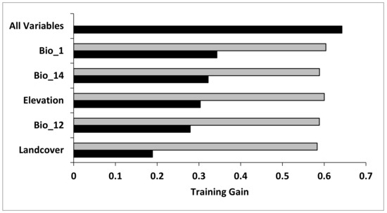
Figure 1.
Jackknife test for evaluating the relative importance of predictor variables. (Annual mean temperature (Bio_1), Annual precipitation (Bio_12), Precipitation of driest month (Bio_14)).
The average training gain gradually declined as variables were removed (Table 2). Test AUC values were significantly better than random (> 0.5 AUC) for all models (0.76–0.88), suggesting little model over-fitting. Using the overlap between 95% confidence intervals, both the average training gain and the average training AUC pointed to the same model as the most parsimonious.
Table 2.
MaxEnt general and reduced models for the cheer pheasant using bioclimatic, topographic and land cover variables.
A five-variable model with elevation, annual mean temperature, annual precipitation, precipitation of driest month, and land cover was the most parsimonious (Table 2). This model had a training AUC of 0.92. Annual precipitation had the greatest contribution (29.9%) to the model, followed by landcover (25.8%), elevation (20.9%), precipitation of the driest month (17.3%), and annual mean temperature (6.1%) (Table 1). Response curves indicated that increased probability of cheer pheasant presence was associated with higher altitude (increasing probability peaking at 2060 m; Figure S2) and land cover categories of needleleaf evergreen forests, grass, bare and rocky ground and croplands (Figure 2).
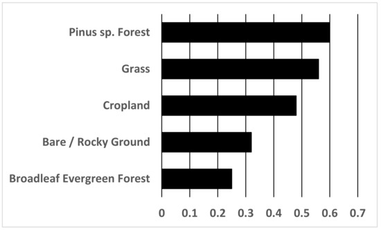
Figure 2.
Predicted preference of cheer in different landcover categories.
There was a strong correlation between known cheer pheasant locations and the continuous probability distribution (Figure 3). We used the five-variable model built from the full set of 99 presence records to create a distribution map of the potential cheer pheasant habitat (Figure 4). The patchy distribution of the species was represented in the model. The total potential cheer pheasant habitat was estimated to cover 3137.9 km2 in the study area (Table 3), of which 91.3% is found in India, 6.3% in Nepal and 2.3% in Pakistan. Most of this potential range in all the range countries lay outside the PA Network (Table 3) and is therefore unprotected. However, human disruptions have a mixed influence on cheer distribution (Figure S3).
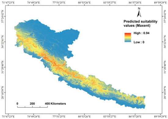
Figure 3.
MaxEnt estimates of the probability of the presence of cheer pheasant in the Himalayan mountains.
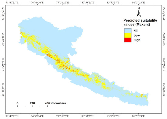
Figure 4.
Distribution and habitat suitability map of cheer pheasant from the best-fitting model.
Table 3.
The estimated extent of cheer pheasant habitat within and outside protected areas.
4. Discussion
The fundamental ecological niche concept was developed by Hutchinson [36] and provided a useful framework pertinent to the biogeographical distribution of species in relation to spatial environmental factors. According to the ecological niche theory, a species’ distribution should be determined mainly by its specific environmental requirements and spatial variation [37]. In this context, our models based on predictor variables can be interpreted as the cheer pheasant’s potential distribution range and are based on simultaneous variations along different axes of the species’ fundamental niche. MaxEnt models do not predict the actual limits of species distribution; however, regions with environmental conditions similar to occurrence localities can be predicted [26]. Our model provided a good prediction of cheer pheasant distribution based on climatic, topographic and habitat variables related to the presence of the species. The selection of environmental variables was based on their demonstrated causal effect on species distribution. In addition to exerting direct physiological effects on the species, the climatic variables are also used to reflect the energy and water availability influencing the ecosystem’s productivity. Topographic variables indirectly impact microclimates within the species ranges [38]. Incorporating land cover variables facilitates the discrimination of species’ habitat preferences [39]. The MaxEnt algorithm derives background or pseudo-absence data from the specified extent of the study area. Hence, the careful delimitation of study area boundaries is an essential consideration in species distribution modelling [40,41]. The limits of our study area were set using the stated global range of the species [2,4].
The full model, based on the complete set of presence records (n = 99), discriminated the distribution of cheer pheasant across its range based on climatic, topographic and habitat variables associated with the presence of the species. The probability for the elevation response curve peaked at 2060 m and then sharply decreased to lower probabilities (Figure S2). The probability of presence was discriminated by the availability of needleleaf evergreen forest, cropland, and grassland with sparse shrubs and trees. Cheer pheasant has been reported to occupy an elevation range between 1445–3050 m [2] in areas interspersed with Chir pine Pinus sp. forests. In many areas of their occupation, the cheer pheasant use croplands and grasslands extensively. The hill grassland habitats of the cheer pheasant are successional and are maintained because of continual disturbance through grazing, grass cutting, and natural or deliberate burning [3,4,5]. Our model predicted that the cheer pheasant had a high preference for grassland and cultivated landscapes.
In the Western Himalayas, grasslands are patchily distributed, and thus the cheer pheasant distribution, which our model depicted. Such patchy distributions of the cheer pheasant are not recent but have been observed much earlier [42,43]. Thus, the extent of cheer pheasant habitat (3137.9 km2) across the three countries is in the form of a broken population comprised of small fragmented sub-populations, a combination of some very small (four to five pairs) and relatively large (>50 pairs) populations.
The bulk of cheer populations across the global range of cheer occur outside the PA network, where they thrive. Only about 15% of this distribution occurs within the Protected Area (PA) network in India, 13% in Pakistan and 40% in Nepal. The cheer seems to have developed an association with humans as some form of continual disturbance in their habitat appears essential to maintain it in that seral stage for it to be suitable. (Figure 5). Too much protection to cheer habitats may render them ‘overgrown’ and thus unsuitable, as demonstrated in Marghala Hills, Pakistan [3]. While apparently, the extent of occupancy for cheer pheasant has mainly remained unchanged, what might be of concern is that the individual habitat patches might have become smaller due to land use changes in the past few decades, reducing the total suitable habitat and, as a result, their abundance.
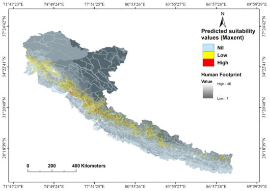
Figure 5.
Habitat suitability map of the Cheer Pheasant overlaid on the human footprint index map.
5. Conservation Implications
The large proportion of cheer pheasant habitat outside protected areas (85%) is also subjected to various forms of anthropogenic effects (Figure 5), such as grazing by livestock, grass cutting and burning and the collection of non-timber forest produce (herbs etc.). These anthropogenic activities have both beneficial and negative impacts. In several grassland areas, in the absence of protection, the grazing and grass-cutting effects are so severe that the habitats are completely denuded and of no use to the species [8]. In Pakistan, the cheer pheasant population remains under the intense pressure of an increasing human population and the associated degradation, clearance, and conversion of habitat into agricultural land [9]. Increased land conversion exacerbated this pressure due to a local shortage of food following the massive earthquake in the parts of Kashmir in 2005 that damaged and destroyed many of the houses in both India and Pakistan on both sides of the Line of Actual Control (LAC). In the rebuilding process, more houses were built than initially present within the habitat of cheer on the Pakistan side of the LAC [9]. In a study undertaken in India to compare the persistence of cheer at some known sites in Himachal Pradesh [44], it was found that while cheer persisted in most sites after three decades, the area of occurrence might have declined in some, again indicating the role of land use conversion in the decline of cheer pheasant habitats. In Nepal, cheer pheasant occurs in substantial numbers outside the protected area network, with 52 of 62 presence localities (former village development committees) lying outside the PA network [11,12,26,45,46] and exposed to pressures of land use change. The threat of hunting is also prevalent across its range, more so outside the protected areas. In Pakistan, birds are killed for meat, and their nests are sought for eggs [9]. Kaul et al. [47] reported that in the Indian states of Himachal Pradesh and Uttarakhand, cheer pheasant was hunted in 67% of the villages around which the species occurred. In western Nepal, snaring, hunting, and egg collection have been reported as threats to the cheer pheasant [6,13]. Additionally, luring birds using the captive cheer is widely practised in far-western Nepal, both within and beyond the PAs network [12]. Land conversion, too, might be responsible for reducing the available habitat of the cheer as found in Himachal Pradesh, India [48].
On the other hand, protected areas afford protection from hunting (if the enforcement is efficient) and land use change. However, occurrence in a protected area is no guarantee, as shown in Nepal, where declines have been reported in Kaligandaki Valley, Rara National Park and Dhorpatan Valley [13]. Reduced human activity within protected areas has also affected cheer [3,5] and other species. Forest succession is suspected of reducing the amount of suitable habitat for Asian elephants (Elephas maximus) within PA systems [49,50]. Such effects have also been seen on other species like the goral (Naemorhedus sp.) [51].
The patchy nature of its habitat represented in our model renders the smaller, isolated populations of cheer pheasant vulnerable to extinction and higher levels of disturbance (e.g., grazing and felling of wooded ravines), especially those exposed to constant and high human pressure. Past surveys also suggest a healthy population of species outside protected areas, substantiating our model prediction (Figure 6). Apart from a few sites that seem to have suffered from over-exploitation, cheer at most sites appears to have benefitted from the inadvertent habitat management by local people, aimed at optimizing resource use and not necessarily the animal numbers [3].
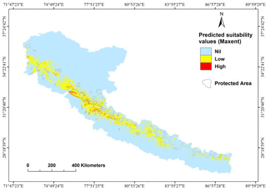
Figure 6.
Protected areas map overlaid with the suitable habitat of the cheer pheasant.
Despite the dangers of local extinctions, we believe that the future of this species lies in areas outside the PA network, and efforts to protect and manage this species will be most successful if the focus of conservation is aimed toward providing protection and improving the management of these areas identified as important cheer pheasant habitats by engaging with local communities to suitably manage habitats and control hunting. Successful pilot projects in Pakistan [52], where the community is protecting cheer breeding habitats, are already ongoing with encouraging results. Similar approaches have been suggested in Nepal [46]. Most actions must focus on reducing or curtailing land use change and the control of hunting. The engagement of local communities in conservation activities can provide outstanding benefits [53], and such options must be explored.
Supplementary Materials
The following supporting information can be downloaded at: https://www.mdpi.com/article/10.3390/d14100785/s1, Figure S1: Map of 99 Cheer pheasant locations used in the analysis. Figure S2: Elevation response curve from the Maxent model. Figure S3: human disturbance response to cheer habitat suitability.
Author Contributions
Conceptualization, R.K. and R.S.K.; methodology, R.S.K., R.S. and R.K.; software, R.S.K. and R.S.; validation, R.S.K., R.S. and R.K.; formal analysis, R.S.K. and R.S.; investigation, R.K., R.S.K., H.B. and M.N.A.; writing—original draft preparation, R.S.K. and R.K.; writing—review and editing, R.K., R.S., M.N.A. and H.B. All authors have read and agreed to the published version of the manuscript.
Funding
This research received no external funding.
Institutional Review Board Statement
The study did not require ethical approval.
Data Availability Statement
Not applicable.
Acknowledgments
The authors are grateful for the technical and financial support from World Pheasant Association and institutions in their respective countries.
Conflicts of Interest
The authors declare no conflict of interest.
References
- IUCN. 2022. The IUCN Red List of Threatened Species. Version 2011-1. Catreus wallichii (Cheer Pheasant). Available online: https://www.iucnredlist.org/species/22679312/112455142# (accessed on 15 July 2022).
- Ali, S.; Ripley, S.D. Handbook of the Birds of India and Pakistan Together with Those of Bangladesh, Nepal, Bhutan and Sri Lanka, Compact Edition; Oxford University Press: Delhi, India, 2022. [Google Scholar]
- Garson, P.J.; Young, L.; Kaul, R. Ecology and conservation of the Cheer Pheasant Catreus wallichii: Studies in wild and the progress of a reintroduction project. Biol. Cons. 1992, 59, 25–35. [Google Scholar] [CrossRef]
- Kaul, R. Ecology of Cheer Pheasant Catreus wallichii in Kumaon Himalaya. Ph.D. Thesis, University of Kashmir, Srinagar, India, 1989. [Google Scholar]
- Kalsi, R.S. Density index and habitat associations of the Cheer Pheasant Catreus wallichi. Report Summer 1998. Fieldwork Tragopan 1998, 10, 16–17. [Google Scholar]
- Subedi, P. Status and Distribution of Cheer Pheasant Catreus Wallichi in Dhorpatan Hunting Reserve, Nepal. Report Submitted to World Pheasant Association and Oriental Bird Club; World Pheasant Association and Oriental Bird Club: Bedford, UK, 2003. [Google Scholar]
- Kalsi, R.S. Status and habitat of Cheer Pheasant in Himachal Pradesh, India—Results of 1997–1998 surveys. Tragopan 2001, 13, 18–24. [Google Scholar]
- Awan, M.N.; Ali, H.; Lee, D.C. Population survey and conservation assessment of the globally threatened Cheer Pheasant (Catreus wallichi) in Jhelum Valley, Pakistan. Chin. J. Zool. Res. 2014, 35, 338. [Google Scholar]
- Fuller, R.A.; Garson, P.J. Pheasants: Status Survey and Conservation Action Plan 2000–2004; IUCN; World Pheasant Association, Reading: Gland, Switzerland; Bedford, UK; pp. 1–66.
- Subedi, P. Monitoring of cheer pheasant Catreus wallichii in Kaligandaki River Valley, Mustang District, Nepal; Report Submitted to National Trust for Nature Conservation, Annapurna Conservation Area Project; Unit Conservation Office: Jomsom, Nepal, 2009. [Google Scholar]
- Basnet, H. Survey of the Cheer Pheasant (Catreus wallichii) in Bajura District Nepal; Report to Oriental Bird Club; Oriental Bird Club: Bedford, UK, 2016. [Google Scholar]
- Basnet, H.; Thapa, T.B.; Subedi, P.; Katuwal, H.B. Decline of the Cheer Pheasant Catreus wallichii in Dhorpatan Hunting Reserve, Nepal. Forktail 2020, 36, 114–116. [Google Scholar]
- Cowley, M.J.R.; Thomas, C.D.; Roy, D.B.; Wilson, R.J.; León-Cortés, J.L.; Gutiérrez, D.; Bulman, C.R.; Quinn, R.M.; Moss, D.; Gaston, K.J. Density-distribution relationships in British butterflies. I. The effect of mobility and spatial scale. J. Anim. Ecol. 2001, 70, 410–425. [Google Scholar] [CrossRef]
- Hanski, I.; Thomas, C.D. Metapopulation dynamics. A spatially explicit model applied to butterflies. Biol. Conserv. 1994, 68, 167–180. [Google Scholar] [CrossRef]
- Phillips, S.J. MaxEnt Software for Species Distribution Modelling. 2005. Available online: http://www.cs.princeton.edu/∼schapire/maxent/ (accessed on 20 July 2022).
- Phillips, S.J.; Anderson, R.P.; Schapire, R.E. Maximum entropy modeling of species geographic distributions. Ecol. Model. 2006, 190, 231–259. [Google Scholar] [CrossRef]
- Phillips, S.J.; Dudik, M. Modeling of species distributions with MaxEnt: New extensions and a comprehensive evaluation. Ecography 2008, 31, 161–175. [Google Scholar] [CrossRef]
- Elith, J.; Phillips, S.J.; Hastie, T.; Dudik, M.; Chee, Y.E.; Yates, C.J. A statistical explanation of MaxEnt for ecologists. Divers. Distrib. 2011, 17, 43–57. [Google Scholar] [CrossRef]
- Karan, P.P. Geographic regions of the Himalayas. Bull. Tibetol. 1966, 3, 5–26. [Google Scholar]
- Hajra, P.K.; Rao, R.R. Distribution of vegetation types in northwest Himalaya with brief remarks on phytogeography and floral resource conservation. Proc. Plant Sci. 1990, 100, 263–277. [Google Scholar] [CrossRef]
- Lillesø, J.-P.B.; Shrestha, T.B.; Dhakal, L.P.; Nayaju, R.P.R.; Shrestha, R. The Map of Potential Vegetation of Nepal—A forestry/agroecological/biodiversity classification system. Forest & Landscape Development and Environment Series 2-2005 and CFC-TIS Document Series No.110. In Forest and Landscape Denmark; The Royal Veterinary and Agricultural University: Copenhagen, Denmark, 2005. [Google Scholar]
- Kalsi, R.S. Status and habitat of the Cheer Pheasant in Himachal Pradesh. Mor 1999, 1, 2–3. [Google Scholar]
- Bisht, M.S.; Phurailatpam, S.; Kathait, B.S. Nesting Ecology and Breeding Success of Cheer Pheasant Catreus wallichii in Garhwal Himalaya, India. J. Bombay Nat. Hist. Soc. 2005, 102, 287–289. [Google Scholar]
- Bisht, M.S.; Phurailatpam, S.; Kathait, B.S.; Dobriyal, A.K.; Chandola-Saklani, A.; Kaul, R. Survey of threatened cheer pheasant Catreus wallichii in Garhwal Himalaya. J. Bombay Nat. Hist. Soc. 2007, 104, 134–139. [Google Scholar]
- Subedi, P. Struggling Cheer Pheasant: A revisit survey in the Kaligandaki valley, Nepal. Ibisbill 2013, 2, 66–74. [Google Scholar]
- Pearson, R.G.; Raxworthy, C.J.; Nakamura, M.; Peterson, A.T. Predicting species distribution from small numbers of occurrence records: A test case using cryptic geckos in Madagascar. J. Biogeogr. 2007, 34, 102–117. [Google Scholar] [CrossRef]
- Hijmans, R.J.; Cameron, S.E.; Parra, J.L.; Jones, P.G.; Jarvis, A. Very high resolution interpolated climate surfaces for global land areas. Int. J. Climatol. 2005, 25, 1965–1978. [Google Scholar] [CrossRef]
- Warren, D.L.; Glor, R.E.; Turelli, M. ENMTools: A toolbox for comparative studies of environmental niche models. Ecography 2010, 33, 607–611. [Google Scholar] [CrossRef]
- ArcMap 10.1. Environmental Science Research Institute (ESRI): Redlands, CA, USA, 2012.
- Global Landcover 2000. Available online: https://forobs.jrc.ec.europa.eu/products/glc2000/products.php> (accessed on 20 July 2022).
- Hansen, M.; DeFries, R.; Townshend, J.R.G.; Sohlberg, R. UMD Global Land Cover Classification, 1 Kilometre, 1.0, Department of Geography; University of Maryland: College Park, MD, USA, 1998; pp. 1981–1994. [Google Scholar]
- Hansen, M.; DeFries, R.; Townshend, J.R.G.; Sohlberg, R. Global land cover classification at 1 km resolution using a decision tree classifier. Int. J. Remote Sens. 2000, 21, 1331–1365. [Google Scholar] [CrossRef]
- Kennedy, C.M.; Oakleaf, J.R.; Theobald, D.M.; Baruch-Mordo, S.; Kiesecker, J. Managing the middle: A shift in conservation priorities based on the global human modification gradient. Glob. Change Biol. 2019, 25, 811–826. [Google Scholar] [CrossRef] [PubMed]
- Brown, J.L. SDMtoolbox: A python-based GIS toolkit for landscape genetic, biogeographic and species distribution model analyses. Methods Ecol. Evol. 2014, 5, 694–700. [Google Scholar] [CrossRef]
- Yost, A.C.; Petersen, S.L.; Gregg, M.; Miller, R. Predictive modeling and mapping Sage grouse (Centrocercus urophasianus) nesting habitat using maximum entropy and a long-term dataset from southern Oregon. Ecol. Inform. 2008, 3, 375–386. [Google Scholar] [CrossRef]
- Hutchinson, G.E. Concluding remarks. Cold Spring Harb. Symp. Quant. Biol. 1957, 22, 415–427. [Google Scholar] [CrossRef]
- Chase, J.M.; Leibold, M.A. Ecological Niches: Linking Classical and Contemporary Approaches; University of Chicago Press: Chicago, IL, USA, 2003. [Google Scholar]
- Guisan, A.; Hofer, U. Predicting reptile distributions at the mesoscale: Relation to climate and topography. J. Biogeogr. 2003, 30, 1233–1243. [Google Scholar] [CrossRef]
- Suárez-Seoane, S.; García de la Morena, E.L.; Morales Prieto, M.B.; Osborne, P.E.; de Juana, E. Maximum entropy niche-based modelling of seasonal changes in Little bustard (Tetrax tetrax) distribution. Ecol. Model. 2008, 219, 17–29. [Google Scholar] [CrossRef]
- Barbet-Massin, M.; Jiguet, F.; Albert, C.H.; Thuiller, W. Selecting pseudoabsences for species distribution models: How, where and how many? Methods Ecol. Evol. 2012, 3, 327–338. [Google Scholar] [CrossRef]
- Smith, A.B. On evaluating species distribution models with random background sites in place of absences when test presences disproportionately sample suitable habitat. Divers. Distrib. 2013, 19, 867–872. [Google Scholar] [CrossRef]
- Hume, A.O.; Marshall, C.H.T. The Game Birds of India, Burma and Ceylon; Acton: Calcutta, India, 1879. [Google Scholar]
- Baker, E.C.S. Game Birds of India, Burma and Ceylon; John Bale and Sons: London, UK, 1930; Volume 3. [Google Scholar]
- Kaul, R.; Poddar, A.; Mohan, L.; Kalsi, R.; Gupta, S.; Nabi, M.; Bhattacharya, T.; Deb, K. Status of Cheer Pheasant and Its Habitats in Some Potential Release Sites in Himachal Pradesh, India; Wildlife Trust of India: Noida, India, 2014. [Google Scholar]
- Acharya, R.; Thapa, S.; Ghimrey, Y. Monitoring of the Cheer Pheasant Catreus Wallichii in Lower Kaligandaki Valley, Mustang Nepal; Report to King Mahendra Trust for Nature Conservation; King Mahendra Trust for Nature Conservation: Kathmandu, Nepal, 2006. [Google Scholar]
- Basnet, H.; Poudyal, L.P. Review on the Distribution of the Cheer Pheasant (Catreus wallichii) in Nepal. Danphe 2017, 26, 2. [Google Scholar]
- Kaul, R.; Hilaluddin Jandrotia, J.S.; McGowan, P.R.J. Hunting of large mammals and pheasants in the western Indian Himalaya. Oryx 2004, 38, 426–431. [Google Scholar] [CrossRef]
- Jolli, V.; Pandit, M.K. Influence of Human Disturbance on the Abundance of Himalayan Pheasant (Aves, Galliformes) in the Temperate Forest of Western Himalaya, India. Vestn. Zool. 2011, 45, 40–47. [Google Scholar] [CrossRef][Green Version]
- De la Torre, J.A.; Wong, E.P.; Lechner, A.M.; Zulaikha, N.; Zawawi, A.; Abdul-Patah, P.; Saaban, S.; Goossens, B.; Campos-Arceiz, A. There will be conflict—Agricultural landscapes are prime, rather than marginal, habitats for Asian elephants. Anim. Conserv. 2021, 24, 720–732. [Google Scholar] [CrossRef]
- Liu, L.I.; Yanfei, J.I.; Hongpei, Y.A.; Aidong, L.U.; Xianming, G.U.; Lifan, W.A.; Li, Z.H. Evaluation of habitat for Asian elephants (Elephas maximus) in Xishuangbanna, Yunan, China. ACTA Theriol. Sin. 2015, 35, 1. [Google Scholar]
- Bhattacharya, T.; Bashir, T.; Poudyal, K.; Sathyakumar, S.; Saha, G.K. Distribution, Occupancy and Activity Patterns of Goral (Nemorhaedus goral) and Serow Capricornis thar) in Khangchendzonga Biosphere Reserve, Sikkim, India. Mammal Study 2012, 37, 173–181. [Google Scholar] [CrossRef]
- Awan, M.N.; Saqib, Z.; Bruner, F.; Lee, D.C.; Pervez, A. Using ensemble modeling to predict breeding habitat of the red-listed Western Tragopan (Tragopan melanocephalus) in the Western Himalayas of Pakistan. Glob. Ecol. Conserv. 2021, 31, e01864. [Google Scholar] [CrossRef]
- Waylen, K.A.; Fischer, A.; Mcgowan, P.J.K. Effect of local cultural context on the success of community-based conservation interventions. Conserv. Biol. 2010, 24, 1119–1129. [Google Scholar] [CrossRef] [PubMed]
Publisher’s Note: MDPI stays neutral with regard to jurisdictional claims in published maps and institutional affiliations. |
© 2022 by the authors. Licensee MDPI, Basel, Switzerland. This article is an open access article distributed under the terms and conditions of the Creative Commons Attribution (CC BY) license (https://creativecommons.org/licenses/by/4.0/).