Abstract
The ongoing climate change and the unprecedented rate of biodiversity loss render the need to accurately project future species distributional patterns more critical than ever. Mounting evidence suggests that not only abiotic factors, but also biotic interactions drive broad-scale distributional patterns. Here, we explored the effect of predator-prey interaction on the predator distribution, using as target species the widespread and generalist grass snake (Natrix natrix). We used ensemble Species Distribution Modeling (SDM) to build a model only with abiotic variables (abiotic model) and a biotic one including prey species richness. Then we projected the future grass snake distribution using a modest emission scenario assuming an unhindered and no dispersal scenario. The two models performed equally well, with temperature and prey species richness emerging as the top drivers of species distribution in the abiotic and biotic models, respectively. In the future, a severe range contraction is anticipated in the case of no dispersal, a likely possibility as reptiles are poor dispersers. If the species can disperse freely, an improbable scenario due to habitat loss and fragmentation, it will lose part of its contemporary distribution, but it will expand northwards.
1. Introduction
Extended human-induced changes have given rise to a more “fragile” world which is getting hotter, with changing precipitation and more frequent extreme weather events [1], e.g., there was an increase of 0.7 °C in average temperature in the last 100 years [2], and a further increase of at least 1.5 °C is anticipated by 2052 [3]. Humans feel the climate change effect through everyday weather [4] and its socio-economic impacts [5,6], while climate change is related to global migration [7,8]. The rate of biodiversity loss is alarming and species have or will be summoned to cope with new climatic conditions by formed new communities. In this context, species shift their behavior [9], phenology [10,11,12], or their range [13], and these changes might allow them to persist and evade extinction. Range shifts include changes in species distributions in different geographic dimensions [14,15,16], with some species suffering range contraction and others exhibiting range expansion [17,18,19]. As the biosphere changes rapidly and in various directions [20], ecologists and biogeographers strive to project the future of species and communities under climate change in order to ensure effective biodiversity conservation and human well-being [21].
Species Distribution Modeling (SDM) [22] is a useful tool to predict climate-change impacts on species distributions (among others [17,23]). SDMs correlate spatially explicit species occurrences with sets of predictors to estimate current distributions and can be projected to other scenarios over time and space [24]. The majority of studies use environmental variables as a set of predictors. This is based on the assumption that the strength of biotic interactions fades at large spatial scales and climate is the preponderant driver of species distributions [24,25]. However, a growing number of studies show that the inclusion of biotic interactions such as competition, facilitation, mutualism and predation into SDMs increase predictive accuracy of the models [26,27,28,29,30,31,32,33,34], suggesting that biotic interactions should be brought into SDMs for more accurate predictions of climate-change impacts [35,36], though caution is required in the interpretation of the observed patterns [37].
Predation is a key biotic interaction shaping structure, dynamics and functioning of ecosystems [38,39,40,41,42], while it contributes to the maintenance of biodiversity [43]. Past global climate change events resulted in species extinctions, shifted species distributions and altered predator-prey interactions, favoring the prevalence of generalists [41]. Ongoing climate change can affect the distribution, population density, behavior, morphology or physiology of both the predator and its prey [42,44,45], inducing shifts in predator-prey dynamics [46], such as disrupted or novel interactions [47] and changes in their strength and frequency [41,48]. However, the first prerequisite for predators and their prey to interact is to overlap in space and in time. Thus, climate change-induced shifts in species distributions might result in spatial or temporal mismatch [49] or overlap into new regions affecting the predator-prey interaction. Given that predator-prey interactions affect the distribution of both the predator and the prey across spatial scales [36], and the strong relationship between a predator and its prey diversity [43], it is critical to take into consideration predator-prey interactions to accurately predict their future distributions under climate change. For instance, Aragón and Sánchez-Fernández [29] found that reptile distribution and richness had a significant effect on the distribution of bird predator in Spain, while Gherghel et al. [31] found that the SDMs predicting sea kraits’ distributional patterns with biotic variables at broad spatial scales were better than the ones including only abiotic variables.
In this study, we explored the role of prey species richness in estimating contemporary distribution and projecting the future distribution of the grass snake Natrix natrix. Reptiles as ectotherms depend on the local temperature to regulate their body temperature and thus, are considered more susceptible to climate change and especially to climate warming [50,51,52]. The grass snake is a trophic generalist and a widespread species ranging from north Africa across Europe up to Scandinavia and east to Lake Baikal, Russia [53]. It benefits from anthropogenic habitats [54] and utilizes anthropogenic heat sources for nesting [55]. Here, using grass snakes we explore the effects of prey species richness and dispersal on the current and future species distribution, as estimated by Species Distribution Modeling of the widespread grass snake.
2. Materials and Methods
2.1. Species Data
We compiled species occurrence data from the Global Biodiversity Information Facility (GBIF) [56] and Sillero et al. [57] as centroids of the atlas grid cells for the grass snake (Natrix natrix) which is widespread in Europe. Natrix natrix taxonomy was recently revised and the species was divided in N. astreptophora found in Spain, Portugal and North Africa, N. helvetica in France, Italy and Great Britain and N. natrix which is distributed east of the Rhine and in the rest of Europe [58,59,60]. Here, we used data of the distribution of Natrix natrix as was newly defined in Europe and thus, occurrences obtained from Sillero et al. [57] were filtered to include species occurrences east of the Rhine and Italy. The grass snake is considered a generalist species. It feeds on amphibians, mostly anurans [61,62,63], but its diet varies with geographical location, habitat or competitor’s presence and may include also small mammals, other reptiles and fish [62,64]. Among its most common prey species are Bufo bufo, Rana temporaria and Lissotriton vulgaris [61,62,63]. Based on this literature, we compiled occurrence data from GBIF [56] for these three species and six more species that were referenced in at least one study and represent various classes (amphibians, other reptiles, small mammals) in Europe. Occurrence data for reptiles-amphibians and mammals were supplemented with occurrences from Sillero et al. [57] and Mitchell-Jones et al. [65] respectively as centroids of the atlas grid cells to ensure a more accurate depiction of the species’ actual distributions. We included in our analysis only georeferenced observations (machine or human) from GBIF and we further tested for invalid records (e.g., countries’ centroids, museums and GBIF headquarters) in the occurrence data with the CoordinateCleaner package [66]. Furthermore, we excluded occurrences with uncertainty higher than the radius of the study’s grid pixels (GBIF field “uncertainty in meters” ≥ 25 km) or outside the species’ range polygons as obtained by the International Union for Conservation of Nature (IUCN) [67] to limit the inclusion of environmental conditions irrelevant to the species’ niche. The comparison with the IUCN range maps was not performed for Natrix natrix as IUCN does not provide spatial data for that species. We accounted for sampling bias by selecting only one random occurrence per pixel [68]. The number of occurrences used in the SDMs, hereafter presences, varied highly per species (see Figure S1).
2.2. Abiotic Variables
We selected as environmental predictors variables related to climate, elevation and water availability to describe current and future environmental conditions (Table S1). All predictors covered the study area which was set between 34° 55’–81° 45’ N and 12° 0’ W–68° 57’ E and were upscaled to a 50 × 50 km grid cell resolution. Specifically, we obtained 19 bioclimatic variables, averaged over the period 1970–2000, provided by the WorldClim 2.1 database [69]. Elevation data were retrieved from the European Digital Elevation Model (EU-DEM) [70]. Furthermore, we estimated the percentage coverage by lakes and the river length included per pixel using data from the CCM River and Catchment Database [71]. Multicollinearity among bioclimatic variables was initially explored by estimating Spearman’s rho correlation coefficient (Table S2). We excluded from the SDM climate predictors that exhibited collinearity, since we examined species with very different physiologies (e.g., endotherms, ectotherms) and we preferred a uniform modeling approach across species [72]. Variance Inflation Factor analysis performed by the usdm package [73] showed strong collinearity between variables, and we included only bioclimatic variables scoring VIF < 5 [74,75,76] in any subsequent analysis (Table S1).
The future bioclimatic variables used in the SDMs were produced by WorldClim 2.1 [69] using downscaled climate projections. These projections were based on the global climate model developed by the Institute Pierre-Simon Laplace (IPSL-CM6A-LR) [77] as a contribution to the Coupled Model Intercomparison Project Phase 6 (CMIP6) [78]. We selected the data for the Shared Socio-Economic Pathway (SSP) 2–4.5 [79] as it represents a modest scenario (“the Middle of the Road” [80]). This scenario predicts a CO2 emissions pick at approximately 44 Gt/year by 2040, followed by a gradual reduction to almost 27 Gt/year by 2080. SSP 2–4.5 estimates an upward trajectory of increase in mean global temperature that will reach 2.5 °C by 2080. We focused on two datasets of bioclimatic variables spanning over two time periods: (i) 2040–2060, hereafter 2060 and (ii) 2060–2080, hereafter 2080.
2.3. Biotic Variables
As a proxy for the trophic interactions of Natrix natrix with its prey we used the prey species richness in the biotic model following Gherghel et al. [31]. Specifically, the potential distribution of each prey species was modeled in the same way as for Natrix natrix for current and future conditions using only abiotic variables (see 2.4. Ensemble species distribution modeling for the methodology followed). Future prey species richness was estimated separately under the unhindered dispersal and no dispersal scenarios; that is, potential future prey distributions were used intact in the first case and limited within their current potential distributions in the latter. We estimated current and future prey species richness as the sum of the prey species’ potential distributions per pixel, which was then used as a predictor in the biotic model of the grass snake.
2.4. Ensemble Species Distribution Modeling
The potential distribution of each species under current and future conditions was estimated with Ensemble Species Distribution modeling using the biomod2 package (version 3.4.6) [81]. Ensemble SDM, by combining predictions from different modeling approaches, can handle prediction variability and results in increased performance [82,83,84,85,86]. We built two models following the same approach: an abiotic model including only abiotic variables, and a biotic model in which the prey species richness was also used as a predictor variable. Prior to model fitting, we selected 1000 pseudo-absences (PAs) from the background data following the surface range envelope strategy (SRE) [87]. The SRE defines the most common environmental conditions where the species occurs and the PAs are drawn randomly outside this envelope. We fitted four algorithms generally classified either as regression-based or machine learning approaches, namely Generalized Linear Models (GLM), Generalized Additive Models (GAM), Flexible Discriminant Analysis (FDA) and Generalized Boosted Models or Boosted Regression Trees (GBM) with the settings shown in Table S3. Each algorithm was run ten times with 70% of the presence-absence data randomly selected, while the other 30% was set aside for cross-validation. The produced models were assessed using the True Skill Statistic (TSS) criterion that ranges between −1 and 1 (perfect score) and reflects the ability of a model to predict correct presences, i.e., sensitivity, and absences, i.e., specificity [88]. We also estimated the Area Under the Curve (AUC) of the Receiver Operating Characteristic (ROC) plot which is a threshold-independent metric that ranges between 0 and 1 with 0.5 indicating that the model discriminates presences randomly and 1 perfectly [89].
The ensemble model for each species was built as a total consensus model using all models and cross-validation runs that satisfy a predetermined evaluation threshold of TSS ≥ 0.7 or, in case of all having TSS < 0.7, with 10% of model runs with the highest TSS [88]. The ensemble model predicted the probability of the presence of each species as the weighted mean of probabilities for the current and future environmental conditions. Specifically, the probability of the presence of each model run complying with the aforementioned criterion contributed to the ensemble probability of presence according to its TSS score. The continuous probability of the presence of the ensemble model was finally transformed to binary using a cut-off value that maximized TSS in order to estimate species vulnerability [90,91]. An overview of the estimation method of grass snake distribution is presented in Figure 1. We estimated the coefficient of variation of the ensemble models and the Multivariate Environmental Suitability Surface (MESS) from dismo package (version 1.3–3) [92] to examine the uncertainty related to the extrapolation outside the range of current environmental conditions used to fit the models. Finally, we evaluated the performance of the SDMs for N. natrix with null models as proposed by Raes and ter Steege [93] to explore whether they differed significantly from random expectations. Specifically, we created 99 null model repetitions for each model type (abiotic and biotic) by randomly selecting points from the study area equal to the number of presences and pseudo-absences used in the real models. We created a frequency histogram with the AUC scores of the null models and assessed the 95% CI upper limit of these values, i.e., selected the 95th AUC value of the ranked scores. All null models ran with the same settings as the real models. The real models were considered significantly better than random if their evaluation scores were above the corresponding 95% CI AUC value of the null models.
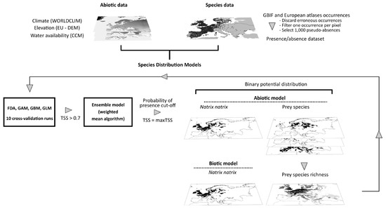
Figure 1.
Summary plot of the workflow followed to estimate potential distribution of Natrix natrix by Species Distribution Modeling. The future distribution of the species was projected using future environmental data in the abiotic model, and environmental data and projected prey species richness in the biotic model, assuming unhindered and no dispersal of Natrix natrix and its prey species.
2.5. Species’ Vulnerability
We adopted commonly used indices to quantify species’ vulnerability to future environmental conditions (among others [94,95]). Specifically, we estimated the relative change in area of potential distribution (change in suitable area, CSA) between current and future time periods as:
and the relative loss of area (loss of suitable area, LSA) as:
where current SA is the number of pixels with currently suitable habitat, future SA is the number of pixels with suitable habitat in the future, and future SA U current SA is the number of pixels with suitable habitat in the present that persists in the future.
All data preparation and analysis were performed in R version 4.0.3 [96].
3. Results
3.1. Performance of the Grass Snake and Prey Species Models and Variable Contribution
The abiotic and the biotic model for the estimation of the grass snake’s current potential distribution were similar in terms of quality as measured by the TSS, AUC and specificity (Table 1). However, the biotic model outperformed slightly the abiotic in sensitivity (Table 1). The ensemble models and the individual models predicting the distribution of prey species performed adequately according to TSS and AUC scores (Table S4, Figure S2). Model uncertainties fluctuated among species (the coefficient of variation ranged between 2.15 and 66.47, Table 1 and Table S4) and in most cases, except for Bufo bufo, uncertainty increased in the Iberian Peninsula and northern Europe (Figure S3). The biotic model for the grass snake exhibited lower uncertainty than the abiotic both as a mean value and across the study areas (Table 1, Figure S3). The MESS maps for Natrix natrix occurrences showed that the extrapolation of model predictions was within the range used to calibrate the model, suggesting reliable predictions in most of the study area (Figure S4). Only in a few areas, mainly at areas of high elevation like the Alps mountains and areas with high aridity like the Iberian Peninsula, extrapolation exceeded this range (Figure S4). Environmental differences between model training and extrapolation were smaller for the abiotic model than the biotic in central and southern Europe (Figure S4). The AUC value of both ensemble models for Natrix natrix was higher than the 95% CI upper limit of the AUC values of the null models suggesting that both models differed significantly from random expectations compared to null models (Table 1).

Table 1.
Scores of evaluation metrics (True-Skill Statistic [TSS], Area Under the Curve (AUC), Sensitivity [%], Specificity [%]) for the specified cut-off value, the coefficient of variation of the ensemble model prediction averaged over the area of prediction, the 95% CI upper limit of AUC values by the null models, range size (number of pixels), the number of occurrences separately for GBIF and the European atlas [4] originally in the datasets, the number of presences kept in the modeling procedure and the variables’ importance (%) for the abiotic and biotic ensemble model for N. natrix rescaled to sum up to 100. The three most important variables are highlighted in bold.
The annual mean temperature was the main predictor of grass snake distribution in the abiotic model (~53%) according to variable importance scores, with the species probability of presence showing a hump-shaped relationship with temperature (Table 1, Figure S5). On the other hand, in the biotic model, prey species richness had the greatest effect on the estimated grass snake distribution (~45%) with the probability of species presence increasing with increasing prey species richness (Table 1, Figure S5). In both models, isothermality contribution on predicting the potential distribution of grass snake was relatively high (~32% and ~26% in the abiotic and biotic model, respectively, approximately hump-shaped relationship) (Table 1, Figure S5). The cumulative contribution of temperature, prey species richness and isothermality was ~85%. In both models, the contribution of any of the remaining variables was smaller than 10% (Table 1). Species response to all variables was similar across model algorithms (FDA, GAM, GBM, GLM) and in both models (Figure S5). Regarding prey species, temperature and isothermality were the strongest predictors of their distribution in the majority of the species (Table S5).
3.2. Potential Distribution of Grass Snake and Its Prey under Current and Future Conditions
The abiotic and biotic models predicted similar potential distribution of grass snakes under current conditions, with the spatial overlap of their estimations being approximately 91% (Table 2). The current potential distribution of the species according to the two models is presented in Figure 2a, and its future projected distribution under different dispersal scenarios in Figure 2b–e. The abiotic model predicted approximately 3% of additional pixels suitable for grass snake and the biotic 6% (Table 2). The inclusion of prey species richness resulted in a slight increase in the potential distribution of the grass snake (Table 1), with its potential distribution spanning a bit further in the south and east of Europe compared to the abiotic model estimation (Figure 2a). Both models predicted presence of the species in Italy and France as predictor variables did not include genetic information based on which N. natrix was divided in N. natrix and N. helvetica [60,97]. Furthermore, the discontinuities of the species distribution in the Balkan Peninsula are possibly impelled by the higher elevation in these areas and the associated decrease of mean annual temperature. The two models exhibited similar patterns of spatial overlap with prey species richness (Figure 3a). The highest overlap was observed in central Europe, the northern Balkans, and Sweden, but at least one prey species is present in almost all of Europe (Figures S6a and S7 for the predicted distribution of each species individually). The spatial overlap of the grass snake’s potential distribution with its prey under future environmental conditions is presented in Figure 3b–e.
Table 2.
Spatial overlap (%) of Natrix natrix potential distribution for current conditions and future projections as predicted by both models and dispersal scenarios and the respective mismatch for each model.
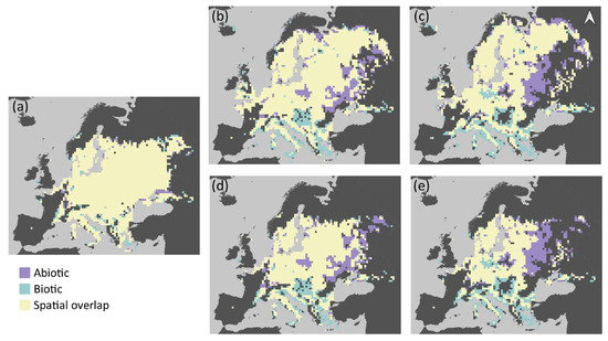
Figure 2.
The potential distribution of grass snake as predicted by the abiotic and biotic Species Distribution Model for different time periods: (a) current time period; and by 2060 and 2080 respectively assuming: (b,c) unhindered dispersal; and (d,e) no dispersal of the species. Scale: 1:110,000,000.
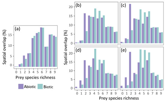
Figure 3.
Spatial overlap (%) of N. natrix predicted potential distribution with prey species richness: (a) under current conditions; and by 2060 and 2080 respectively assuming: (b,c) the unhindered dispersal scenario; (d,e) the no dispersal scenario.
In the no dispersal scenario, the two models predict similar future potential distribution of the grass snake (Table 2). The species distribution in central Europe becomes more discontinuous with time according to both models (Figure 2d,e). However, the grass snake is anticipated to lose parts of its current distribution in the east, according to the biotic model, and in the south, according to the abiotic model (Figure 4d,e). Furthermore, the biotic model estimates larger losses than the abiotic, i.e., almost 26% and 42.5% of its current distribution by 2060 (Figure 2d and Figure 4c) and 2080 (Figure 2e and Figure 4d) respectively. In this case, prey species were also subjected to the no dispersal limitation and are expected to suffer range contraction. In the future, the grass snake overlap with its prey differs between models (Figure 3d,e). The abiotic model predicts losses of grass snake distribution in the south, where prey species richness is anticipated to be higher compared to eastern Europe (Figure 2d,e and Figure S6c,e), and thus, lower co-occurrence of predator with high prey species richness is expected (Figure 3d,e). On the other hand, the biotic model predicts losses of both predator and prey species in the same areas, i.e., in the east (Figure 2d,e and Figure S6c,e), resulting in an increased overlap of the predator with at least four prey species (Figure 3d,e).
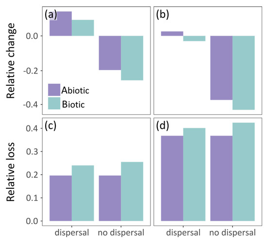
Figure 4.
Grass snake’s vulnerability to climate warming according to the abiotic and biotic model assuming unhindered and no dispersal of the species. Vulnerability is measured as follows: (a,b) relative change (CSA); and (c,d) relative loss (LSA) of its potential distribution by: (a,c) 2060; and (b,d) 2080.
In the unhindered dispersal scenario, there was a slightly lower disagreement in the predictions of the future potential distribution of grass snake provided by the abiotic and biotic model than the no dispersal scenario (Table 2). In this case, the grass snake still counts losses south and east depending on the model but expands further to the north according to both models (~3% increase and 3% decrease in range size by 2080 for the abiotic and biotic model respectively; Figure 2c and Figure 4b). In the biotic model, the species exhibits patchy distribution in the east, while discontinuities are predicted by the abiotic model in the south, analogous to the no dispersal scenario (Figure 2b,c). Apart from the northward expansion expected for the predator and its prey in the unhindered dispersal scenario (Figure 2b,c and Figure S6b,d), prey species richness distribution within the predator distribution was similar in both dispersal scenarios (Figure 3b–e).
4. Discussion
Species distributions at broad scales are considered to be driven by abiotic factors, where biotic interactions, that manifest at local scales and diminish at broad scales, add only noise to SDMs [25]. However, a series of studies have demonstrated that biotic interactions affect species distributions across spatial scales [26,27,31,32,33]. Our results showed that the Species Distribution Model of Natrix natrix, including prey species richness, had similar performance with the one including only abiotic variables. Both models performed well, i.e., differentiated strongly species presences and absences.
The similar performance of biotic and abiotic SDM might be due to the type of interaction explored here, i.e., predator-prey, and the feeding ecology of the grass snake, i.e., a generalist snake. The effect of biotic interactions across scales depends on the type of interaction, and a positive interaction is more probable to scale up than a negative interaction [98,99]. Predator-prey is a consumer-resource interaction, meaning that is positive for the predator and negative for the prey, and if it scales up it depends on the net effect of the interaction [98]. Furthermore, the role of biotic interactions on species distribution has been related to the degree of a species’ specialization [26,100,101]. The grass snake’s trophic generalization might explain why the inclusion of prey species richness did not improve the SDM. Studies that reported that predator-prey interaction is imprinted on the species distribution at broader spatial scales focused primarily on trophic specialists, e.g., [29,31]. For instance, Gherghel et al. [31], who proposed the incorporation of prey species richness into SDMs, used as target species sea kraits, i.e., snakes that are trophic specialists, and found that the inclusion of prey species richness improved the model’s quality only slightly.
Temperature was the top driver of the distributional pattern of grass snake in the abiotic model, while isothermality also played a role. Reptiles depend strongly on the local temperature to regulate their body temperature [102], with other aspects such as metabolic rate, sex determination, and nesting depending on temperature as well. Temperature is a strong limiting factor in the northern part of their distribution (cold physiological limit) [103,104] and other factors, e.g., biotic interactions drive the southern limit of their distribution [105,106]. It seems that the presence of the grass snake is favored up to a mean annual temperature ranging approximately 4–11 °C (this depends on the model used to estimate its distribution), and also from smaller levels of isothermality, perhaps in order to retain activity. Therefore, the grass snake can survive in a wide array of thermal conditions, as it is also reflected by its wide distribution, i.e., from warmer conditions, like those prevailing in the Mediterranean, to cold, e.g., Scandinavia. Although the biotic SDM did not perform better than the abiotic, the prey species richness was the most important driver of grass snake distribution, contributing approximately 45% to the SDM. The distribution of the majority of prey species and the predator (according to the abiotic model) is driven by similar predictors (temperature and isothermality). These species seem to thrive in the same areas dictated by their thermal biology, and this perhaps can explain the similar performance of abiotic and biotic SDMs, i.e., although the species interact, the similar environmental niches might partially mask the imprint of biotic interaction on the broad-scale distribution of this generalist predator.
Both models predicted shifts of the grass snake’s distribution under the climate change scenario assuming unlimited dispersal, and losses assuming no dispersal. Under the no dispersal scenario, the species is projected to suffer range contraction by 2080, while under the unhindered dispersal scenario, the losses of current distribution will be compensated by expansion to the north. According to the abiotic model with no dispersal, range contraction is inevitable in the face of climate change with the species losing a large part of its current distribution in the Balkan Peninsula by 2060 and approximately 37% of its current distribution by 2080. However, if the species can disperse freely, it is expected to expand into new areas northwards and eastwards; in the latter case, losing simultaneously to the south until 2080. Note that the unhindered dispersal scenario used here is in congruence with the limited dispersal assumed for amphibians by Thuiller et al. [107], i.e., 20 km/year, and a suggestion made by Smith and Green [108], i.e., 10 km/year for amphibian dispersal ability, although reptiles are considered poor dispersers [17,109] with reported maximum dispersal of 3 km to our knowledge [110]. In the case of a biotic model, grass snake is anticipated to retain the southern parts of its distribution, but to become extinct in the east. Assuming no dispersal, the species will suffer a range of contraction (similar to the abiotic model), but it will expand northwards if it can disperse. The two models exhibited differences regarding the distribution in the south which were sharpened by 2080. Specifically, the biotic model predicted a distribution with a further southern edge than that of the abiotic model. Perhaps, although future climatic conditions exceed the physiological limits of the species there, the presence of some prey mitigates them. This is in congruence with the finding that the southern range limits of amphibians and reptiles are determined by species interactions (see Cunningham et al. [105] and references therein).
Snakes and reptiles, in general, are considered to globally decline [51,109] due to climate change and induced changes (e.g., habitat loss, prey availability), while regional declines in grass snakes have been reported [111]. Even assuming that the species can disperse unhindered based on their dispersal ability, habitat loss and fragmentation and land-use changes, which are among the main drivers of the global decline of amphibians and reptiles [112], might render the expanded suitable space inaccessible [113]. Therefore, the dispersal ability of species and connectivity will crucially affect the future distribution of the species [17,114]. It seems that climate warming along with the ongoing habitat fragmentation [115] minimizes the reptiles’ chance to move to areas with suitable environmental conditions [17,110]. This is vividly depicted by the range contraction projected by the SDMs assuming no dispersal. Furthermore, global warming might favor reptiles by increasing the available suitable area for them but can negatively impact phenology-related aspects resulting in higher metabolic rates and skewed sex ratio due to their temperature-dependent sex determination [50,115,116]. Although adaptations to these changes have “rescued” reptile species from historic climate warming events, a timely adaptation is not the most probable scenario [50,117,118,119].
5. Conclusions
We found a similarly good performance of the biotic and the abiotic Species Distribution Model predicting the distribution of the generalist Natrix natrix. However, the prey species richness was the top driver of grass snake distribution, highlighting the role of the prey availability in shaping species distribution. Temperature and isothermality played a significant role in shaping the grass snake distribution in all cases. The abiotic and the biotic model predicted a northward shift of the species distribution under climate change assuming unlimited dispersal, but severe range contractions in the case of no dispersal. Our results highlighted that biotic interactions and dispersal ability are game-changers in future projections of species distributions and should be included in SDMs. However, they differ widely among taxonomic groups and regions and cannot be collectively modeled for different taxonomic groups. Thus, more taxon and region-specific studies are needed if we want to predict a species’ response to climate warming and develop effective conservation strategies.
Supplementary Materials
The following are available online at https://www.mdpi.com/article/10.3390/d13040169/s1, Table S1: The predictors considered for the species distribution modeling. Table S2: Spearman’s rho correlation coefficients between bioclimatic variables. Table S3: The models used for the ensemble modeling and the associated parameter settings. Table S4: The total number of occurrences and separately for GBIF and the European atlases originally in the datasets, the number of presences kept in the modeling procedure, True Skill Statistic (TSS), Area Under the Curve (AUC), sensitivity and specificity scores for the presented cut-off value for each prey species and the coefficient of variation of the ensemble model prediction for each species averaged over the area of prediction. Table S5: Variable importance (%) for the prediction of each prey species probability of presence in the abiotic ensemble species distribution model., Figure S1: Presences used in the modeling process for each species. Figure S2: Scores of True Skill Statistic (TSS) and Area Under the Curve (AUC) for each individual model, prey species and model type (abiotic and biotic) for Natrix natrix. Figure S3: Coefficients of variation (standard deviation/mean) of the predictions for the ensemble species distribution model of each species and model type (abiotic and biotic) for Natrix natrix. Figure S4: Multivariate environmental suitability surface maps (MESS) of the predictors included in the abiotic and the biotic model for current environmental conditions for Natrix natrix. Figure S5: Predicted response curves from the different algorithms that were used in the individual and ensemble models for Natrix natrix. Figure S6: Predicted prey species richness under current environmental conditions and by 2060 and 2080 respectively according to unhindered dispersal scenario and no dispersal scenario. Figure S7: Predicted distribution of each prey species according to an abiotic ensemble species distribution model.
Author Contributions
Conceptualization, D.-E.M., M.L. and S.P.S.; methodology, D.-E.M. and M.L.; software, D.-E.M. and M.L.; validation, D.-E.M., M.L. and S.P.S.; formal analysis, D.-E.M. and M.L.; investigation, D.-E.M., M.L. and S.P.S.; resources, S.P.S.; data curation, D.-E.M. and M.L.; writing—original draft preparation, D.-E.M. and M.L.; writing—review and editing, D.-E.M., M.L. and S.P.S.; visualization, D.-E.M. and M.L.; supervision, S.P.S.; project administration, S.P.S.; funding acquisition, S.P.S. All authors have read and agreed to the published version of the manuscript.
Funding
This research is co-financed by Greece and the European Union (European Social Fund ESF) through the Operational Programme «Human Resources Development, Education and Lifelong Learning 2014 2020» in the context of the project «The species area relationship reversed Estimation of the minimum area that encompasses S species» (MIS 5047923).
Institutional Review Board Statement
Not applicable.
Informed Consent Statement
Not applicable.
Data Availability Statement
Publicly available datasets were analyzed in this study. This data can be found here: https://www.gbif.org/; http://na2re.ismai.pt/; https://www.european-mammals.org/php/mapmaker.php; https://www.iucnredlist.org/; https://worldclim.org/; https://www.eea.europa.eu/data-and-maps/data/copernicus-land-monitoring-service-eu-dem; https://ec.europa.eu/jrc/en/publication/eur-scientific-and-technical-research-reports/ccm-river-and-catchment-database-version-20-analysis-tools.
Acknowledgments
We would like to thank the anonymous reviewers for their very helpful comments. This research is co-financed by Greece and the European Union (European Social Fund ESF) through the Operational Programme «Human Resources Development, Education and Lifelong Learning 2014 2020» in the context of the project «The species area relationship reversed Estimation of the minimum area that encompasses S species» (MIS 5047923).
Conflicts of Interest
The authors declare no conflict of interest.
References
- Thornton, P.K.; Ericksen, P.J.; Herrero, M.; Challinor, A.J. Climate variability and vulnerability to climate change: A review. Glob. Chang. Biol. 2014, 20, 3313–3328. [Google Scholar] [CrossRef]
- IPCC. Climate Change 2013: The Physical Science Basis: Working Group I Contribution to the Fifth Assessment Report of the Intergovernmental Panel on Climate Change; Cambridge University Press: Cambridge, UK, 2014. [Google Scholar]
- Masson-Delmotte, V.; Zhai, P.; Pörtner, H.-O.; Roberts, D.; Skea, J.; Shukla, P.R.; Pirani, A.; Moufouma-Okia, W.; Péan, C.; Pidcock, R. Global warming of 1.5 °C. IPCC Spec. Rep. Impacts Glob. Warm. 2018, 1, 1–9. [Google Scholar]
- Sippel, S.; Meinshausen, N.; Fischer, E.M.; Székely, E.; Knutti, R. Climate change now detectable from any single day of weather at global scale. Nat. Clim. Chang. 2020, 10, 35–41. [Google Scholar] [CrossRef]
- Tol, R.S. The economic impacts of climate change. Rev. Environ. Econ. Policy 2018, 12, 4–25. [Google Scholar] [CrossRef]
- Tol, R.S.J. The economic effects of climate change. J. Econ. Perspect. 2009, 23, 29–51. [Google Scholar] [CrossRef]
- Myers, N. Environmental refugees: A growing phenomenon of the 21st century. Philos. Trans. R. Soc. Lond. B Biol. Sci. 2002, 357, 609–613. [Google Scholar] [CrossRef] [PubMed]
- Biermann, F.; Boas, I. Preparing for a warmer world: Towards a global governance gystem to protect climate refugees. Glob. Environ. Politics 2010, 10, 60–88. [Google Scholar] [CrossRef]
- Beever, E.A.; Hall, L.E.; Varner, J.; Loosen, A.E.; Dunham, J.B.; Gahl, M.K.; Smith, F.A.; Lawler, J.J. Behavioral flexibility as a mechanism for coping with climate change. Front. Ecol. Environ. 2017, 15, 299–308. [Google Scholar] [CrossRef]
- Cohen, J.M.; Lajeunesse, M.J.; Rohr, J.R. A global synthesis of animal phenological responses to climate change. Nat. Clim. Chang. 2018, 8, 224–228. [Google Scholar] [CrossRef]
- Peñuelas, J.; Filella, I. Phenology feedbacks on climate change. Science 2009, 324, 887–888. [Google Scholar] [CrossRef]
- Urban, M.C.; Richardson, J.L.; Freidenfelds, N.A. Plasticity and genetic adaptation mediate amphibian and reptile responses to climate change. Evol. Appl. 2014, 7, 88–103. [Google Scholar] [CrossRef]
- Parmesan, C. Ecological and evolutionary responses to recent climate change. Annu. Rev. Ecol. Evol. Syst. 2006, 37, 637–669. [Google Scholar] [CrossRef]
- Parmesan, C.; Yohe, G. A globally coherent fingerprint of climate change impacts across natural systems. Nature 2003, 421, 37–42. [Google Scholar] [CrossRef] [PubMed]
- Lenoir, J.; Svenning, J.C. Climate-related range shifts—A global multidimensional synthesis and new research directions. Ecography 2015, 38, 15–28. [Google Scholar] [CrossRef]
- Chen, I.-C.; Hill, J.K.; Ohlemüller, R.; Roy, D.B.; Thomas, C.D. Rapid range shifts of species associated with high levels of climate warming. Science 2011, 333, 1024–1026. [Google Scholar] [CrossRef]
- Araújo, M.B.; Thuiller, W.; Pearson, R.G. Climate warming and the decline of amphibians and reptiles in Europe. J. Biogeogr. 2006, 33, 1712–1728. [Google Scholar] [CrossRef]
- Popescu, V.D.; Rozylowicz, L.; Cogalniceanu, D.; Niculae, I.M.; Cucu, A.L. Moving into protected areas? Setting conservation priorities for Romanian reptiles and amphibians at risk from climate change. PLoS ONE 2013, 8, e79330. [Google Scholar] [CrossRef]
- Somero, G.N. The physiology of climate change: How potentials for acclimatization and genetic adaptation will determine ‘winners’ and ‘losers’. J. Exp. Biol. 2010, 213, 912–920. [Google Scholar] [CrossRef]
- Corlett, R.T. The Anthropocene concept in ecology and conservation. Trends Ecol. Evol. 2015, 30, 36–41. [Google Scholar] [CrossRef]
- Pecl, G.T.; Araujo, M.B.; Bell, J.D.; Blanchard, J.; Bonebrake, T.C.; Chen, I.C.; Clark, T.D.; Colwell, R.K.; Danielsen, F.; Evengard, B.; et al. Biodiversity redistribution under climate change: Impacts on ecosystems and human well-being. Science 2017, 355. [Google Scholar] [CrossRef] [PubMed]
- Guisan, A.; Zimmermann, N.E. Predictive habitat distribution models in ecology. Ecol. Model. 2000, 135, 147–186. [Google Scholar] [CrossRef]
- Guisan, A.; Thuiller, W. Predicting species distribution: Offering more than simple habitat models. Ecol. Lett. 2005, 8, 993–1009. [Google Scholar] [CrossRef]
- Pearson, R.G.; Dawson, T.P. Predicting the impacts of climate change on the distribution of species: Are bioclimate envelope models useful? Glob. Ecol. Biogeogr. 2003, 12, 361–371. [Google Scholar] [CrossRef]
- Soberon, J.; Nakamura, M. Niches and distributional areas: Concepts, methods, and assumptions. Proc. Natl. Acad. Sci. USA 2009, 106 (Suppl. S2), 19644–19650. [Google Scholar] [CrossRef]
- Araújo, M.B.; Luoto, M. The importance of biotic interactions for modelling species distributions under climate change. Glob. Ecol. Biogeogr. 2007, 16, 743–753. [Google Scholar] [CrossRef]
- Heikkinen, R.K.; Luoto, M.; Virkkala, R.; Pearson, R.G.; Körber, J.-H. Biotic interactions improve prediction of boreal bird distributions at macro-scales. Glob. Ecol. Biogeogr. 2007, 16, 754–763. [Google Scholar] [CrossRef]
- Gotelli, N.J.; Graves, G.R.; Rahbek, C. Macroecological signals of species interactions in the Danish avifauna. Proc. Natl. Acad. Sci. USA 2010, 107, 5030–5035. [Google Scholar] [CrossRef] [PubMed]
- Aragón, P.; Sánchez-Fernández, D. Can we disentangle predator-prey interactions from species distributions at a macro-scale? A case study with a raptor species. Oikos 2013, 122, 64–72. [Google Scholar] [CrossRef]
- Staniczenko, P.P.A.; Sivasubramaniam, P.; Suttle, K.B.; Pearson, R.G. Linking macroecology and community ecology: Refining predictions of species distributions using biotic interaction networks. Ecol. Lett. 2017, 20, 693–707. [Google Scholar] [CrossRef]
- Gherghel, I.; Brischoux, F.; Papeş, M. Using biotic interactions in broad-scale estimates of species’ distributions. J. Biogeogr. 2018, 45, 2216–2225. [Google Scholar] [CrossRef]
- Flores-Tolentino, M.; Garcia-Valdes, R.; Saenz-Romero, C.; Avila-Diaz, I.; Paz, H.; Lopez-Toledo, L. Distribution and conservation of species is misestimated if biotic interactions are ignored: The case of the orchid Laelia speciosa. Sci. Rep. 2020, 10, 9542. [Google Scholar] [CrossRef]
- Tsiftsis, S.; Djordjević, V. Modelling sexually deceptive orchid species distributions under future climates: The importance of plant–pollinator interactions. Sci. Rep. 2020, 10. [Google Scholar] [CrossRef]
- de Araújo, C.B.; Marcondes-Machado, L.O.; Costa, G.C.; Silman, M. The importance of biotic interactions in species distribution models: A test of the Eltonian noise hypothesis using parrots. J. Biogeogr. 2014, 41, 513–523. [Google Scholar] [CrossRef]
- Botkin, D.B.; Saxe, H.; Araújo, M.B.; Betts, R.; Bradshaw, R.H.W.; Cedhagen, T.; Chesson, P.; Dawson, T.P.; Etterson, J.R.; Faith, D.P.; et al. Forecasting the effects of global warming on biodiversity. Bioscience 2007, 57, 227–236. [Google Scholar] [CrossRef]
- Wisz, M.S.; Pottier, J.; Kissling, W.D.; Pellissier, L.; Lenoir, J.; Damgaard, C.F.; Dormann, C.F.; Forchhammer, M.C.; Grytnes, J.A.; Guisan, A.; et al. The role of biotic interactions in shaping distributions and realised assemblages of species: Implications for species distribution modelling. Biol. Rev. Camb. Philos. Soc. 2013, 88, 15–30. [Google Scholar] [CrossRef]
- Dormann, C.F.; Bobrowski, M.; Dehling, D.M.; Harris, D.J.; Hartig, F.; Lischke, H.; Moretti, M.D.; Pagel, J.; Pinkert, S.; Schleuning, M.; et al. Biotic interactions in species distribution modelling: 10 questions to guide interpretation and avoid false conclusions. Glob. Ecol. Biogeogr. 2018, 27, 1004–1016. [Google Scholar] [CrossRef]
- Ives, A.R.; Cardinale, B.J.; Snyder, W.E. A synthesis of subdisciplines: Predator-prey interactions, and biodiversity and ecosystem functioning. Ecol. Lett. 2004, 8, 102–116. [Google Scholar] [CrossRef]
- Cadotte, M.W.; Fukami, T. Dispersal, spatial scale, and species diversity in a hierarchically structured experimental landscape. Ecol. Lett. 2005, 8, 548–557. [Google Scholar] [CrossRef] [PubMed]
- Schmitz, O.J. Effects of predator hunting mode on grassland ecosystem function. Science 2008, 319, 952–954. [Google Scholar] [CrossRef] [PubMed]
- Blois, J.L.; Zarnetske, P.L.; Fitzpatrick, M.C.; Finnegan, S. Climate change and the past, present, and future of biotic interactions. Science 2013, 341, 499–504. [Google Scholar] [CrossRef] [PubMed]
- Laws, A.; Joern, A. Density mediates grasshopper performance in response to temperature manipulation and spider predation in tallgrass prairie. Bull. Entomol. Res. 2017, 107, 261. [Google Scholar] [CrossRef]
- Sandom, C.; Dalby, L.; Flojgaard, C.; Kissling, W.D.; Lenoir, J.; Sandel, B.; Trojelsgaard, K.; Ejrnaes, R.; Svenning, J.C. Mammal predator and prey species richness are strongly linked at macroscales. Ecology 2013, 94, 1112–1122. [Google Scholar] [CrossRef]
- Bastille-Rousseau, G.; Schaefer, J.A.; Lewis, K.P.; Mumma, M.A.; Ellington, E.H.; Rayl, N.D.; Mahoney, S.P.; Pouliot, D.; Murray, D.L. Phase-dependent climate-predator interactions explain three decades of variation in neonatal caribou survival. J. Anim. Ecol. 2016, 85, 445–456. [Google Scholar] [CrossRef] [PubMed]
- Bretagnolle, V.; Terraube, J. Predator–Prey Interactions and Climate Change; Oxford University Press: Oxford, UK, 2019; pp. 199–220. [Google Scholar] [CrossRef]
- Bastille-Rousseau, G.; Gibbs, J.P.; Yackulic, C.B.; Frair, J.L.; Cabrera, F.; Rousseau, L.-P.; Wikelski, M.; Kümmeth, F.; Blake, S. Animal movement in the absence of predation: Environmental drivers of movement strategies in a partial migration system. Oikos 2017, 126, 1004–1019. [Google Scholar] [CrossRef]
- Rockwell, R.F.; Gormezano, L.J.; Koons, D.N. Trophic matches and mismatches: Can polar bears reduce the abundance of nesting snow geese in western Hudson Bay? Oikos 2011, 120, 696–709. [Google Scholar] [CrossRef]
- Harley, C.D. Climate change, keystone predation, and biodiversity loss. Science 2011, 334, 1124–1127. [Google Scholar] [CrossRef] [PubMed]
- Schweiger, O.; Settele, J.; Kudrna, O.; Klotz, S.; Kuhn, I. Climate change can cause spatial mismatch of trophically interacting species. Ecology 2008, 89, 3472–3479. [Google Scholar] [CrossRef]
- Bickford, D.; Howard, S.D.; Ng, D.J.J.; Sheridan, J.A. Impacts of climate change on the amphibians and reptiles of Southeast Asia. Biodivers. Conserv. 2010, 19, 1043–1062. [Google Scholar] [CrossRef]
- Reading, C.; Luiselli, L.; Akani, G.; Bonnet, X.; Amori, G.; Ballouard, J.-M.; Filippi, E.; Naulleau, G.; Pearson, D.; Rugiero, L. Are snake populations in widespread decline? Biol. Lett. 2010, 6, 777–780. [Google Scholar] [CrossRef]
- Paaijmans, K.P.; Heinig, R.L.; Seliga, R.A.; Blanford, J.I.; Blanford, S.; Murdock, C.C.; Thomas, M.B. Temperature variation makes ectotherms more sensitive to climate change. Glob. Chang. Biol. 2013, 19, 2373–2380. [Google Scholar] [CrossRef] [PubMed]
- Beebe, T.; Griffiths, R. Amphibians and Reptiles: A Natural History of the British Herpetofauna; Harper Collins: London, UK, 2000. [Google Scholar]
- Kabisch, K. Natrix natrix (Linnaeus, 1758)–Ringelnatter. In Handbuch der Reptilien und Amphibien Europas; AULA-Verlag: Wiebelsheim, Germany, 1999; Volume 3, pp. 513–580. [Google Scholar]
- Löwenborg, K.; Kärvemo, S.; Tiwe, A.; Hagman, M. Agricultural by-products provide critical habitat components for cold-climate populations of an oviparous snake (Natrix natrix). Biodivers. Conserv. 2012, 21, 2477–2488. [Google Scholar] [CrossRef]
- GBIF. GBIF Home Page. Available online: https://www.gbif.org (accessed on 24 October 2020).
- Sillero, N.; Campos, J.; Bonardi, A.; Corti, C.; Creemers, R.; Crochet, P.-A.; Crnobrnja Isailović, J.; Denoël, M.; Ficetola, G.F.; Gonçalves, J.; et al. Updated distribution and biogeography of amphibians and reptiles of Europe. Amphib.-Reptil. 2014, 35, 1–31. [Google Scholar] [CrossRef]
- Pokrant, F.; Kindler, C.; Ivanov, M.; Cheylan, M.; Geniez, P.; Böhme, W.; Fritz, U. Integrative taxonomy provides evidence for the species status of the Ibero-Maghrebian grass snakeNatrix astreptophora. Biol. J. Linn. Soc. 2016, 118, 873–888. [Google Scholar] [CrossRef]
- Kindler, C.; de Pous, P.; Carranza, S.; Beddek, M.; Geniez, P.; Fritz, U. Phylogeography of the Ibero-Maghrebian red-eyed grass snake (Natrix astreptophora). Org. Divers. Evol. 2017, 18, 143–150. [Google Scholar] [CrossRef]
- Kindler, C.; Gracia, E.; Fritz, U. Extra-Mediterranean glacial refuges in barred and common grass snakes (Natrix helvetica, N. natrix). Sci. Rep. 2018, 8, 1821. [Google Scholar] [CrossRef] [PubMed]
- Gregory, P.T.; Isaac, L.A. Food habits of the grass snake in southeastern England: Is Natrix natrix a generalist predator? J. Herpetol. 2004, 38, 88–95. [Google Scholar] [CrossRef]
- Šukalo, G.; Đorđević, S.; Gvozdenović, S.; Simović, A.; Anđelković, M.; Blagojević, V.; Tomović, L. Intra-and inter-population variability of food preferences of two Natrix species on the Balkan Peninsula. Herpetol. Conserv. Biol. 2014, 9, 123–136. [Google Scholar]
- Nilson, G.; AndrÉN, C. Morphology and taxonomic status of the grass snake, Natrix natrix (L.) (Reptilia, Squamata, Colubridae) on the island of Gotland, Sweden. Zool. J. Linn. Soc. 1981, 72, 355–368. [Google Scholar] [CrossRef]
- Luiselli, L.; Filippi, E.; Capula, M. Geographic variation in diet composition of the grass snake (Natrix natrix) along the mainland and an island of italy: The effects of habitat type and interference with potential competitors. Herpetol. J. 2005, 15, 221–230. [Google Scholar]
- Mitchell-Jones, A.J.; Amori, G.; Bogdanowicz, W.; Krystufek, B.; Reijnders, P.; Spitzenberger, F.; Stubbe, M.; Thissen, J.; Vohralik, V.; Zima, J. The Atlas of European Mammals; Academic Press: London, UK, 1999; Volume 3. [Google Scholar]
- Zizka, A.; Silvestro, D.; Andermann, T.; Azevedo, J.; Duarte Ritter, C.; Edler, D.; Farooq, H.; Herdean, A.; Ariza, M.; Scharn, R.; et al. CoordinateCleaner: Standardized Cleaning of Occurrence Records from Biological Collection Databases. R Package Version 2.0-18. 2019. Available online: https://github.com/ropensci/CoordinateCleaner (accessed on 25 October 2020). [CrossRef]
- IUCN. The IUCN Red List of Threatened Species. Available online: https://www.iucnredlist.org (accessed on 24 October 2020).
- Beck, J.; Böller, M.; Erhardt, A.; Schwanghart, W. Spatial bias in the GBIF database and its effect on modeling species’ geographic distributions. Ecol. Inform. 2014, 19, 10–15. [Google Scholar] [CrossRef]
- Fick, S.E.; Hijmans, R.J. WorldClim 2: New 1-km spatial resolution climate surfaces for global land areas. Int. J. Climatol. 2017, 37, 4302–4315. [Google Scholar] [CrossRef]
- European Digital Elevation Model (EU-DEM), Version 1. 1; Copernicus Land Monitoring Services: Copenhagen, Denmark, 2019. [Google Scholar]
- CCM River and Catchment Database; European Commission—JRC: Ispra, Italy, 2007.
- Merow, C.; Smith, M.J.; Silander, J.A. A practical guide to MaxEnt for modeling species’ distributions: What it does, and why inputs and settings matter. Ecography 2013, 36, 1058–1069. [Google Scholar] [CrossRef]
- Naimi, B.; Hamm, N.A.S.; Groen, T.A.; Skidmore, A.K.; Toxopeus, A.G. Where is positional uncertainty a problem for species distribution modelling? Ecography 2014, 37, 191–203. [Google Scholar] [CrossRef]
- Neter, J.; Kutner, M.H.; Nachtsheim, C.J.; Wasserman, W. Applied Linear Statistical Models; McGraw-Hill: New York, NY, USA, 1996. [Google Scholar]
- Dormann, C.F.; Elith, J.; Bacher, S.; Buchmann, C.; Carl, G.; Carré, G.; Marquéz, J.R.G.; Gruber, B.; Lafourcade, B.; Leitão, P.J.; et al. Collinearity: A review of methods to deal with it and a simulation study evaluating their performance. Ecography 2013, 36, 27–46. [Google Scholar] [CrossRef]
- Becker, J.-M.; Ringle, C.M.; Sarstedt, M.; Völckner, F. How collinearity affects mixture regression results. Mark. Lett. 2014, 26, 643–659. [Google Scholar] [CrossRef]
- Boucher, O.; Servonnat, J.; Albright, A.L.; Aumont, O.; Balkanski, Y.; Bastrikov, V.; Bekki, S.; Bonnet, R.; Bony, S.; Bopp, L.; et al. Presentation and evaluation of the IPSL-CM6A-LR climate model. J. Adv. Modeling Earth Syst. 2020, 12. [Google Scholar] [CrossRef]
- Eyring, V.; Bony, S.; Meehl, G.A.; Senior, C.A.; Stevens, B.; Stouffer, R.J.; Taylor, K.E. Overview of the Coupled Model Intercomparison Project Phase 6 (CMIP6) experimental design and organization. Geosci. Model Dev. 2016, 9, 1937–1958. [Google Scholar] [CrossRef]
- Fricko, O.; Havlik, P.; Rogelj, J.; Klimont, Z.; Gusti, M.; Johnson, N.; Kolp, P.; Strubegger, M.; Valin, H.; Amann, M.; et al. The marker quantification of the Shared Socioeconomic Pathway 2: A middle-of-the-road scenario for the 21st century. Glob. Environ. Chang. 2017, 42, 251–267. [Google Scholar] [CrossRef]
- Riahi, K.; van Vuuren, D.P.; Kriegler, E.; Edmonds, J.; O’Neill, B.C.; Fujimori, S.; Bauer, N.; Calvin, K.; Dellink, R.; Fricko, O.; et al. The Shared Socioeconomic Pathways and their energy, land use, and greenhouse gas emissions implications: An overview. Glob. Environ. Chang. 2017, 42, 153–168. [Google Scholar] [CrossRef]
- Thuiller, W.; Georges, D.; Engler, R.; Breiner, F. Biomod2: Ensemble Platform for Species Distribution Modeling; R Package Version 3.4.6. 2020. Available online: https://CRAN.R-project.org/package=biomod2 (accessed on 26 October 2020).
- Marmion, M.; Parviainen, M.; Luoto, M.; Heikkinen, R.K.; Thuiller, W. Evaluation of consensus methods in predictive species distribution modelling. Divers. Distrib. 2009, 15, 59–69. [Google Scholar] [CrossRef]
- Crossman, N.D.; Bass, D.A. Application of common predictive habitat techniques for post-border weed risk management. Divers. Distrib. 2007, 14, 213–224. [Google Scholar] [CrossRef]
- Aguirre-Gutierrez, J.; Carvalheiro, L.G.; Polce, C.; van Loon, E.E.; Raes, N.; Reemer, M.; Biesmeijer, J.C. Fit-for-purpose: Species distribution model performance depends on evaluation criteria—Dutch Hoverflies as a case study. PLoS ONE 2013, 8, e63708. [Google Scholar] [CrossRef] [PubMed]
- Comte, L.; Grenouillet, G.; Robertson, M. Species distribution modelling and imperfect detection: Comparing occupancy versus consensus methods. Divers. Distrib. 2013, 19, 996–1007. [Google Scholar] [CrossRef]
- Araujo, M.B.; New, M. Ensemble forecasting of species distributions. Trends Ecol. Evol. 2007, 22, 42–47. [Google Scholar] [CrossRef]
- Barbet-Massin, M.; Jiguet, F.; Albert, C.H.; Thuiller, W. Selecting pseudo-absences for species distribution models: How, where and how many? Methods Ecol. Evol. 2012, 3, 327–338. [Google Scholar] [CrossRef]
- Allouche, O.; Tsoar, A.; Kadmon, R. Assessing the accuracy of species distribution models: Prevalence, kappa and the true skill statistic (TSS). J. Appl. Ecol. 2006, 43, 1223–1232. [Google Scholar] [CrossRef]
- Fielding, A.H.; Bell, J.F. A review of methods for the assessment of prediction errors in conservation presence/absence models. Environ. Conserv. 1997, 38–49. [Google Scholar] [CrossRef]
- Liu, C.; White, M.; Newell, G.; Pearson, R. Selecting thresholds for the prediction of species occurrence with presence-only data. J. Biogeogr. 2013, 40, 778–789. [Google Scholar] [CrossRef]
- Jiménez-Valverde, A.; Lobo, J.M. Threshold criteria for conversion of probability of species presence to either–or presence–absence. Acta Oecol. 2007, 31, 361–369. [Google Scholar] [CrossRef]
- Elith, J.H.; Graham, C.P.; Anderson, R.; Dudík, M.; Ferrier, S.; Guisan, A.J.; Hijmans, R.; Huettmann, F.R.; Leathwick, J.; Lehmann, A.; et al. Novel methods improve prediction of species’ distributions from occurrence data. Ecography 2006, 29, 129–151. [Google Scholar] [CrossRef]
- Raes, N.; ter Steege, H. A null-model for significance testing of presence-only species distribution models. Ecography 2007, 30, 727–736. [Google Scholar] [CrossRef]
- Zhang, J.; Nielsen, S.E.; Chen, Y.; Georges, D.; Qin, Y.; Wang, S.-S.; Svenning, J.-C.; Thuiller, W. Extinction risk of North American seed plants elevated by climate and land-use change. J. Appl. Ecol. 2017, 54, 303–312. [Google Scholar] [CrossRef]
- Thuiller, W.; Lavergne, S.; Roquet, C.; Boulangeat, I.; Lafourcade, B.; Araujo, M.B. Consequences of climate change on the tree of life in Europe. Nature 2011, 470, 531–534. [Google Scholar] [CrossRef] [PubMed]
- R Core Team. R: A Language and Environment for Statistical Computing; R Foundation for Statistical Computing: Vienna, Austria, 2020. [Google Scholar]
- Kindler, C.; Chevre, M.; Ursenbacher, S.; Bohme, W.; Hille, A.; Jablonski, D.; Vamberger, M.; Fritz, U. Hybridization patterns in two contact zones of grass snakes reveal a new Central European snake species. Sci. Rep. 2017, 7, 7378. [Google Scholar] [CrossRef]
- Araújo, M.B.; Rozenfeld, A. The geographic scaling of biotic interactions. Ecography 2014, 37, 406–415. [Google Scholar] [CrossRef]
- Belmaker, J.; Zarnetske, P.; Tuanmu, M.-N.; Zonneveld, S.; Record, S.; Strecker, A.; Beaudrot, L. Empirical evidence for the scale dependence of biotic interactions. Glob. Ecol. Biogeogr. 2015, 24, 750–761. [Google Scholar] [CrossRef]
- Bateman, B.L.; VanDerWal, J.; Williams, S.E.; Johnson, C.N. Biotic interactions influence the projected distribution of a specialist mammal under climate change. Divers. Distrib. 2012, 18, 861–872. [Google Scholar] [CrossRef]
- Jaeschke, A.; Bittner, T.; Jentsch, A.; Reineking, B.; Schlumprecht, H.; Beierkuhnlein, C. Biotic interactions in the face of climate change: A comparison of three modelling approaches. PLoS ONE 2012, 7, e51472. [Google Scholar] [CrossRef]
- Porter, W.P.; Gates, D.M. Thermodynamic equilibria of animals with environment. Ecol. Monogr. 1969, 39, 227–244. [Google Scholar] [CrossRef]
- Sunday, J.M.; Bates, A.E.; Dulvy, N.K. Global analysis of thermal tolerance and latitude in ectotherms. Proc. Biol. Sci. 2011, 278, 1823–1830. [Google Scholar] [CrossRef] [PubMed]
- Sunday, J.M.; Bates, A.E.; Dulvy, N.K. Thermal tolerance and the global redistribution of animals. Nat. Clim. Chang. 2012, 2, 686–690. [Google Scholar] [CrossRef]
- Cunningham, H.R.; Rissler, L.J.; Buckley, L.B.; Urban, M.C. Abiotic and biotic constraints across reptile and amphibian ranges. Ecography 2016, 39, 1–8. [Google Scholar] [CrossRef]
- Schemske, D.W.; Mittelbach, G.G.; Cornell, H.V.; Sobel, J.M.; Roy, K. Is there a latitudinal gradient in the importance of biotic interactions? Annu. Rev. Ecol. Evol. Syst. 2009, 40, 245–269. [Google Scholar] [CrossRef]
- Thuiller, W.; Gueguen, M.; Renaud, J.; Karger, D.N.; Zimmermann, N.E. Uncertainty in ensembles of global biodiversity scenarios. Nat. Commun. 2019, 10, 1446. [Google Scholar] [CrossRef] [PubMed]
- Smith, A.M.; Green, D.M. Dispersal and the metapopulation paradigm in amphibian ecology and conservation: Are all amphibian populations metapopulations? Ecography 2005, 28, 110–128. [Google Scholar] [CrossRef]
- Gibbons, J.W.; Scott, D.E.; Ryan, T.J.; Buhlmann, K.A.; Tuberville, T.D.; Metts, B.S.; Greene, J.L.; Mills, T.; Leiden, Y.; Poppy, S. The global decline of reptiles, déjà vu amphibians. Bioscience 2000, 50, 653–666. [Google Scholar] [CrossRef]
- Clauzel, C.; Godet, C. Combining spatial modeling tools and biological data for improved multispecies assessment in restoration areas. Biol. Conserv. 2020, 250, 108713. [Google Scholar] [CrossRef]
- Hagman, M.; Elmberg, J.; Kärvemo, S.; Löwenborg, K. Grass snakes (Natrix natrix) in Sweden decline together with their anthropogenic nesting-environments. Herpetol. J. 2012, 22, 199–202. [Google Scholar]
- Winter, M.; Fiedler, W.; Hochachka, W.M.; Koehncke, A.; Meiri, S.; De la Riva, I. Patterns and biases in climate change research on amphibians and reptiles: A systematic review. R. Soc. Open Sci. 2016, 3, 160158. [Google Scholar] [CrossRef] [PubMed]
- Sahlean, T.C.; Gherghel, I.; Papeş, M.; Strugariu, A.; Zamfirescu, Ş.R. Refining climate change projections for organisms with low dispersal abilities: A case study of the Caspian whip snake. PLoS ONE 2014, 9, e91994. [Google Scholar] [CrossRef]
- Sahlean, T.C.; Papeș, M.; Strugariu, A.; Gherghel, I. Ecological corridors for the amphibians and reptiles in the Natura 2000 sites of Romania. Sci. Rep. 2020, 10, 1–11. [Google Scholar] [CrossRef] [PubMed]
- Todd, B.D.; Willson, J.D.; Gibbons, J.W. The global status of reptiles and causes of their decline. Ecotoxicol. Amphib. Reptiles 2010, 47, 67. [Google Scholar] [CrossRef]
- Böhm, M.; Cook, D.; Ma, H.; Davidson, A.D.; García, A.; Tapley, B.; Pearce-Kelly, P.; Carr, J. Hot and bothered: Using trait-based approaches to assess climate change vulnerability in reptiles. Biol. Conserv. 2016, 204, 32–41. [Google Scholar] [CrossRef]
- Mitchell, N.J.; Janzen, F.J. Temperature-dependent sex determination and contemporary climate change. Sex. Dev. 2010, 4, 129–140. [Google Scholar] [CrossRef] [PubMed]
- Bodensteiner, B.L.; Agudelo-Cantero, G.A.; Arietta, A.A.; Gunderson, A.R.; Muñoz, M.M.; Refsnider, J.M.; Gangloff, E.J. Thermal adaptation revisited: How conserved are thermal traits of reptiles and amphibians? J. Exp. Zool. Part A Ecol. Integr. Physiol. 2021, 335, 173–194. [Google Scholar] [CrossRef] [PubMed]
- Lawler, J.J.; Shafer, S.L.; Bancroft, B.A.; Blaustein, A.R. Projected climate impacts for the amphibians of the Western Hemisphere. Conserv. Biol. 2010, 24, 38–50. [Google Scholar] [CrossRef] [PubMed]


Publisher’s Note: MDPI stays neutral with regard to jurisdictional claims in published maps and institutional affiliations. |
© 2021 by the authors. Licensee MDPI, Basel, Switzerland. This article is an open access article distributed under the terms and conditions of the Creative Commons Attribution (CC BY) license (https://creativecommons.org/licenses/by/4.0/).