Article

Dynamics of a Predator–Prey Model with the Effect of Oscillation of Immigration of the Prey

by
Jawdat Alebraheem
Department of Mathematics, College of Science Al Zufli, Majmaah University, Majmaah 11952, Saudi Arabia
Diversity 2021, 13(1), 23; https://doi.org/10.3390/d13010023
Submission received: 11 November 2020 / Revised: 2 January 2021 / Accepted: 5 January 2021 / Published: 10 January 2021
(This article belongs to the Special Issue Predator–Prey Ecology and Conservation in ‘Novel’ Environments)

Abstract

:
In this article, the use of predator-dependent functional and numerical responses is proposed to form an autonomous predator–prey model. The dynamic behaviors of this model were analytically studied. The boundedness of the proposed model was proven; then, the Kolmogorov analysis was used for validating and identifying the coexistence and extinction conditions of the model. In addition, the local and global stability conditions of the model were determined. Moreover, a novel idea was introduced by adding the oscillation of the immigration of the prey into the model which forms a non-autonomous model. The numerically obtained results display that the dynamic behaviors of the model exhibit increasingly stable fluctuations and an increased likelihood of coexistence compared to the autonomous model.

1. Introduction

Organism population dynamics evolve through the changing sizes of populations. These dynamics take many different forms. Predator–prey interactions are primary forms that elucidate the population dynamics of many species. These interactions have received significant attention from many researchers [1,2,3,4,5,6]. Lotka [7] and Volterra [8] proposed the first model in this direction. Their model is considered to be the foundation stone for studying the dynamics of predator–prey interactions. Moreover, nonlinear differential equations form the mathematical basis for describing predator–prey interactions. The Lotka–Volterra model has been enhanced by many researchers to make it more realistic, and considering various ecological processes in doing so, see for instance [9,10].
Functional and numerical responses are considered as the central components for building predator–prey models; they also play a crucial role for describing the dynamic behaviors of these models [9]. The functional response is defined as the consumption rate of the prey by a predator, while the numerical response is the result of prey consumption on the predator density. In this context, the functional response was first suggested by Solomon [11] in 1949. A decade later, it was studied and classified into three types by the Canadian ecologist Holling, namely Holling types I, II and III [12]. The Holling type II was developed by Crowley and Martin [13], by adding terms that make the functional response depend on the prey and predator abundance, which takes into account the predator interference, so that makes it more realistic.
In the literature, few studies have investigated the Crowley–Martin type of responses in predator–prey models using different concepts to study the dynamics of these models. Upadhyay and Naji [14] used Holling type II and the Crowley–Martin type with a three-species food chain model to discuss the dynamics of the model. Ali and Jazar [15] studied the global dynamics of a modified Leslie–Gower predator–prey model using the Crowley–Martin functional response and Holling type II as the numerical response. Stage-structured predator–prey models with the Crowley–Martin type have been widely considered [16,17,18] to discuss the dynamics of these models. Alebraheem and Abu-Hassan [19] investigated the seasonality in the predator–prey model with the Crowley–Martin type to identify complex dynamic behaviors. Mortoja et al. [20] used the Crowley–Martin type in a delayed predator–prey model involving disease in the prey population. Moreover, the Crowley–Martin type was used with a discrete predator–prey system to study the complex dynamics that lead to chaos [21,22]. In addition, the Crowley–Martin type has been investigated in stochastic predator–prey models [23,24] for studying the asymptotic properties of these models.
Different factors play an important role affecting the dynamic behaviors of predator–prey interactions, which may come from environmental or human factors such as refuge, migration, immigration, and oscillations. Immigration has effects on the stability of predator–prey interactions as shown in [25,26]. Oscillations that come from seasonal impacts play an important role affecting the dynamic behaviors of predator–prey interactions as shown in previous studies [27,28,29]. Despite the aforementioned efforts, no investigation has been conducted on oscillations in immigration that may affect the dynamics of predator–prey interactions.
In this article, Crowley–Martin-type functional and numerical responses are utilized to form an autonomous predator–prey model. The boundedness and validation of the model are presented. The dynamic behaviors of the model are studied by using some qualitative analysis, which involves stability analysis, and obtaining the coexistence and extinction conditions. In addition, a novel idea is introduced through adding the oscillation of the immigration of the prey into a predator–prey model, which forms a non-autonomous model. The comparison by using the numerical simulations between the two models are shown to present the change in dynamic behaviors and explaining the effects that come from investigating the oscillation of immigration of the prey.
The remainder of the article is set out as follows. Section 2 introduces the predator–prey model without the oscillation of immigration and proves the boundedness of the model. Section 3 presents the theoretical analysis of the model, which is divided to three subsections. Section 3.1 validates the model using Kolmogorov conditions. Section 3.2 introduces the existence of equilibrium points. Section 3.3 introduces the stability analysis of the model. Section 4 presents the numerical simulations that show the changing dynamic behaviors of this model with the oscillation of immigration of the prey. Section 5 presents a final discussion and conclusion.

2. Model and Boundedness without Oscillation of the Immigration

The autonomous predator–prey model with the Crowley–Martin functional and numerical responses is described as follows:
d x d t = ζ x ( 1 x k ) c x y 1 + h x + σ y + h σ x y = x M ( x , y ) ,
d y d t = μ y + γ c x y 1 + h x + σ y + h σ x y = y N ( x , y ) ,
which is subjected to the following initial conditions:
x ( 0 ) = x 0 ,   y ( 0 ) = y 0 .
Here, ζ represents the prey growth rate, k is the carrying capacity in the absence of predation, and μ is the predator death rate. The parameters of the functional and numerical responses are as follows: c denotes the efficiency of searching and capturing the predator, and γ indicates the efficiency of converting the consumed prey into predator births. Moreover, h represents the handling time, and σ is the magnitude of interference among predators.
Theorem 1.
For model (1) and any given positive initial value, the solution of t 0 will be in R + 2 and is ultimately bounded.
Proof. 
Suppose ( x ( t ) , y ( t ) ) to be any solution of model (1) with initial conditions (2). Let E ( t ) = x ( t ) + 1 γ y ( t ) . The time derivative of function E is:
d E d t = d x d t + 1 γ d y d t
d E d t = ( ζ ( 1 x k ) c y 1 + h x + σ y + h σ x y ) x + ( μ γ + c x 1 + h x + σ y + h σ x y ) y .
Equation (3) becomes:
d E d t = ( ζ ( 1 x k ) ) x + μ γ y .
Because all the parameters are positive, and the initiating solutions remain in R + 2 , the following could be assumed:
d E d t ( ζ ( 1 x k ) ) x μ E .
Hence:
max { R + ζ x ( 1 x k ) } = ζ k 4 .
Substituting (5) in (4), the following is obtained:
d E d t ζ k 4 μ E ,
which implies:
lim   sup   t E ( t ) ζ k 4 μ .
Consequently, x ( t ) and y ( t ) are ultimately bounded. □

3. Theoretical Analysis of the Model without Immigration

3.1. Kolmogorov Analysis

Kolmogorov analysis was used to validate the predator–prey system and obtain the coexistence and extinction conditions. The Kolmogorov analysis is a group of conditions that are summarized and explained in Freedman [30] and Sigmund [31]. Therefore, the following conditions are used:
(1)
If the number of predators increases and the number of prey is fixed, then the prey and predator growth rate decrease. The factors that express these conditions are represented as follows:
M y < 0 ,
d N d y < 0 .
Equation (8) can be interpreted as the predators competing for the same source. Therefore, these conditions are applied in model (1) as follows:
M y = c ( 1 + h x ) ( 1 + σ y ) 2 < 0
N y = γ c σ x ( 1 + h x ) ( 1 + σ y ) 2 < 0
The conditions (9) and (10) of model (1) are always negative because the values of the variables and parameters are positive.
(2)
The model includes the environment carrying capacity. The following condition of model (1) is attained:
ρ > 0   M ( ρ , 0 ) = 0 ,   then   ρ = k
(3)
The model has a minimum prey value, even in the case of a small predator population. The following condition of model (1) is attained:
η > 0   N ( η , 0 ) = 0 ,   then   η = μ γ c μ h
(4)
The predators coexist with the prey if the following condition is satisfied:
ρ > η
Thus, the following condition of model (1) is obtained:
k γ c k μ h > μ
Condition (14) represents the coexistence condition. However, if this condition is not satisfied, then:
k γ c k μ h μ
and the predators become extinct.
Many researchers have studied coexistence and extinction dynamics [32,33,34,35,36,37,38]. On account of their importance, the following definitions are presented:
Definition 1.
If x ( 0 ) > 0 and l i m t x ( t ) > 0 , then x ( t ) coexists. However, the geometrical definition is that each path of the differential equations is ultimately bounded afar from the coordinate planes.
Definition 2.
Extinction is analytically defined such that, if x ( 0 ) > 0 and l i m t x ( t ) = 0 , then x ( t ) become extinct. Meanwhile, the geometrical definition is that the path of the differential equations touches the coordinate planes.
From the Kolmogorov analysis, the following propositions are concluded:
Proposition 1.
If condition (14) is satisfied, then the predator coexists with the prey.
Corollary 1.
The predator become extinct under condition (15).

3.2. Existence of Equilibrium Points

Model (1) has three non-negative equilibrium points, which are biologically feasible because E 0 = ( 0 ,   0 ) , E 1 = ( k ,   0 ) , and E 2 = ( x ¯ ,   y ¯ ) . Equilibrium points E 0 and E 1 exist without conditions. Equilibrium point E 2 exists as explained in Proposition 1. E 2 is obtained by finding the positive real root of the following algebraic equations:
ζ ( 1 x ¯ k ) c   y ¯ 1 + h x ¯ + σ   y ¯ + h σ x ¯   y ¯ = 0
μ + γ c x ¯ 1 + h x ¯ + σ   y ¯ + h σ x ¯   y ¯ = 0
The following analysis is introduced to show the existence of x ¯ and y ¯ .
From Equation (16), consider:
M ( x , y ) = ζ ( 1 x ¯ k ) c   y ¯ 1 + h x ¯ + σ   y ¯ + h σ x ¯   y ¯ = 0
The following is noticed:
When x ¯ = 0 , then y ¯ = ζ c ζ σ = y ¯ i . It is clear that y ¯ i > 0 under the following condition:
c > ζ σ
(i)
When y ¯ = 0 , then x ¯ = k = x ¯ i . Then, it has x ¯ i > 0 always without any condition.
(ii)
d   y ¯ d x ¯ = M / x ¯ M /   y ¯ = ζ k + c h   y ¯ ( 1 + h x ¯ ) 2 ( 1 + σ   y ¯ ) c ( 1 + h x ¯ ) ( 1 + σ   y ¯ ) 2
Then d y ¯ d x ¯ < 0 , if it has the following condition:
ζ ( 1 + h x ¯ ) 2 ( 1 + σ   y ¯ ) > c h k   y ¯
Using the above analysis, it was shown that isocline (18) passed through the points ( x ¯ i ,   0 ) and ( 0 ,   y ¯ i ) ; and in Equation (18), y ¯ is a decreasing function of x ¯ under conditions (19) and (20).
From Equation (17), let:
N ( x , y ) = μ + γ c x ¯ 1 + h x ¯ + σ   y ¯ + h σ x ¯   y ¯ = 0
The following is noticed:
(i)
When y ¯ = 0 , then x ¯ = μ γ c h μ = x ¯ i i . It is clear that x ¯ i i > 0 under the following condition:
γ c > μ h
(ii)
d   y ¯ d x ¯ = N / x N /   y ¯ = 1 + σ   y ¯ σ x ( 1 + h x ) > 0
This explains that isocline (21) is passing through the point ( x ¯ i i ,   0 ) under the condition (22), and it always has a positive slope, so in Equation (21), y ¯ increases as x ¯ increases.
Through the above analysis, it is attained that the two isoclines (18) and (21) intersect at a unique point ( x ¯ ,   y ¯ ) if:
x ¯ i i < x ¯ i
Proposition 2.
If conditions (19), (20), (22) and (23) are satisfied, then model (1) has a unique positive equilibrium point.

3.3. Local and Global Stability Analysis

The qualitative analysis of differential equations is essential in population dynamics [39] because they follow the dynamic behaviors of populations and an exact solution is quite difficult [40]. The local and global stability of equilibrium points E 0 , E 1 , and E 2 are studied using the following theorems.
Theorem 2.
Trivial equilibrium point E 0 = ( 0 ,   0 ) is a saddle point.
Proof. 
The Jacobian matrix of E 0 is yielded by
V ( E 0 ) = ( ζ 0 0 μ )
Using the corresponding Jacobian matrix, it was obtained that, with eigenvalues λ 1 = ζ > 0 , E 0 is always positive, and with λ 2 = μ < 0 , it is always negative. Therefore, E 0 is a saddle point. □
Theorem 3.
Predator-free equilibrium point E 1 = ( k ,   0 ) is locally asymptotically stable and subjected to the following condition:
μ + μ h k > γ c k
Proof. 
The Jacobian matrix of E 1 is:
V ( E 1 ) = ( ζ ( c + h c k ) ( 1 + h k ) 2 0 μ + γ c k 1 + h k )
Through the corresponding Jacobian matrix, it is attained that the eigenvalue λ 1 = ζ and is always negative. Meanwhile, λ 2 = μ + γ c k 1 + h k will be negative if the condition (24) is satisfied.
Therefore, E 1 is locally asymptotically stable under condition (24). However, if the condition (24) is not satisfied, then E 1 is a saddle point.
Theorem 4.
Coexistence equilibrium point E 2 = ( x ¯ , y ¯ ) is locally asymptotically stable subjected to the following condition:
h c x ¯ y ¯ ( 1 + h x ) 2 ( 1 + σ y ) < ζ x ¯ k + γ c σ x ¯   y ¯ ( 1 + h x ) ( 1 + σ y ) 2
Proof. 
The Jacobian matrix of E 2 is:
V ( E 2 ) = ( x ¯ ( ζ k h c y ¯ ( 1 + h x ) 2 ( 1 + σ y ) ) x ¯ ( c ( 1 + h x ) ( 1 + σ y ) 2 ) y ¯ ( γ c ( 1 + h x ) 2 ( 1 + σ y ) ) y ¯ ( γ c σ x ¯ ( 1 + h x ) ( 1 + σ y ) 2 ) )
Using the corresponding Jacobian matrix, E 2 is locally asymptotically stable under condition (25). □
Corollary 2.
If condition (25) is violated, then the coexistence equilibrium point E 2 = ( x ¯ , y ¯ ) presents a stable fluctuated dynamic behavior.
Theorem 5.
Predator-free equilibrium point E 1 = ( k ,   0 ) is globally asymptotically stable in the interior of R + 2 under the condition (24).
Proof. 
Define the Lyapunov function of E 1 :
L = ( x k k ln ( x k ) ) + y γ ,
where L is a continuously differentiable real valued function defined in R + 2 . Therefore, we have:
d L d t = ζ ( 1 x k ) d x d t + 1 γ d y d t ,
d L d t = ( x k ) x x [ ζ ζ x k c y 1 + h x + σ y + h σ x y ] + y γ [ μ + γ c x 1 + h x + σ y + h σ x y ] ,
d L d t = r k ( x k ) 2 c x y 1 + h x + σ y + h σ x y + k c y 1 + h x + σ y + h σ x y μ γ y + c x y 1 + h x + σ y + h σ x y ,
d L d t = r k ( x k ) 2 + k c y 1 + h x + σ y + h σ x y μ γ y ,
d L d t = r k ( x k ) 2 + ( k c 1 + h x + σ y + h σ x y μ γ ) y .
If condition (24) is satisfied, then d L d t < 0 for any point in R + 2 . □
Theorem 6.
Coexistence equilibrium point E 2 is globally asymptotically stable in the interior of R + 2 under condition (25).
Proof. 
Consider that G ( x , y ) = 1 x y , where G represents a Dulac function. It is the C 1 function in the interior of R + 2 and A = { { ( x , y ) | x > 0 ,   y > 0 } .
T 1 ( x , y ) = ζ x ( 1 x k ) c x y 1 + h x + σ y + h σ x y ,
and:
T 2 ( x , y ) = μ y + γ c x y 1 + h x + σ y + h σ x y .
Thus:
( G T 1 , G T 2 ) = ( G N 1 ) x + ( G N 2 ) y = ζ y k + h c + c h σ y ( 1 + h x + σ y + h σ x y ) 2 ( γ c σ γ c h σ x ( 1 + h x + σ y + h σ x y ) 2 ) .
As x ¯ > 0 , y ¯ > 0 , and all the parameters are positive, then < 0 under condition (25). By the Bendixson–Dulac criterion, E 2 is globally asymptotically stable in the interior of R + 2 under the condition (25). □

4. Model with Oscillation of Immigration

The non-autonomous predator–prey model with Crowley–Martin functional and numerical responses with oscillation of immigration of the prey is described as follows:
d x d t = ζ x ( 1 x k ) c x y 1 + h x + σ y + h σ x y + i   ( 1 + ϵ sin ( w t ) )
d y d t = μ y + γ c x y 1 + h x + σ y + h σ x y .
which is subjected to the following initial conditions:
x ( 0 ) = x 0 ,   y ( 0 ) = y 0 .
where i the number of prey immigrants [25,26], ϵ represents the degree of fluctuation. The parameter w is the angular frequency of the fluctuations.

5. Numerical Simulations

The numerical simulations of models (1) and (32) were performed to show the change in dynamic behaviors and explain the effects that come from investigating the oscillation of the immigration of the prey. “NDsolve” command in the MATHEMATICA 11.3 software package was used to solve the models numerically for different sets of the hypothetical values of the parameters. They were assumed to satisfy the theoretical side of each case, but the values of the initial conditions were fixed for all cases. In Section 3, the theoretical analysis presents two different dynamics of the model (1), so two different sets of the hypothetical values of the parameters were selected for representing two different dynamic behaviors that were steady state and fluctuated, respectively. There is an important question that can be asked in this context: how does adding the oscillation of immigration of the prey affect the dynamic behaviors? Figure 1, Figure 2, Figure 3, Figure 4, Figure 5, Figure 6, Figure 7, Figure 8, Figure 9 and Figure 10 illustrate the different kinds of graphs that are used to explain these cases; time series figures and zero-growth isoclines with phase plane trajectory figures are plotted to show the dynamic behaviors and trajectories comprehensively, as well as the cross-sectional picture of zero-growth isoclines with phase plane trajectories for each figure is introduced to give clear picture of the dynamic behavior.
The initial conditions for all cases are supposed as follows:
x ( 0 ) = 3 ,   y ( 0 ) = 2 .
The first set of parameter values is considered as follows:
ζ = 2 ,   k = 4 ,   c = 2 ,   h = 1.3 ,   σ = 0.9 ,   μ = 0.4 ,   γ = 1.2 ,   ϵ = 0.75 ,   w = 0.5 .
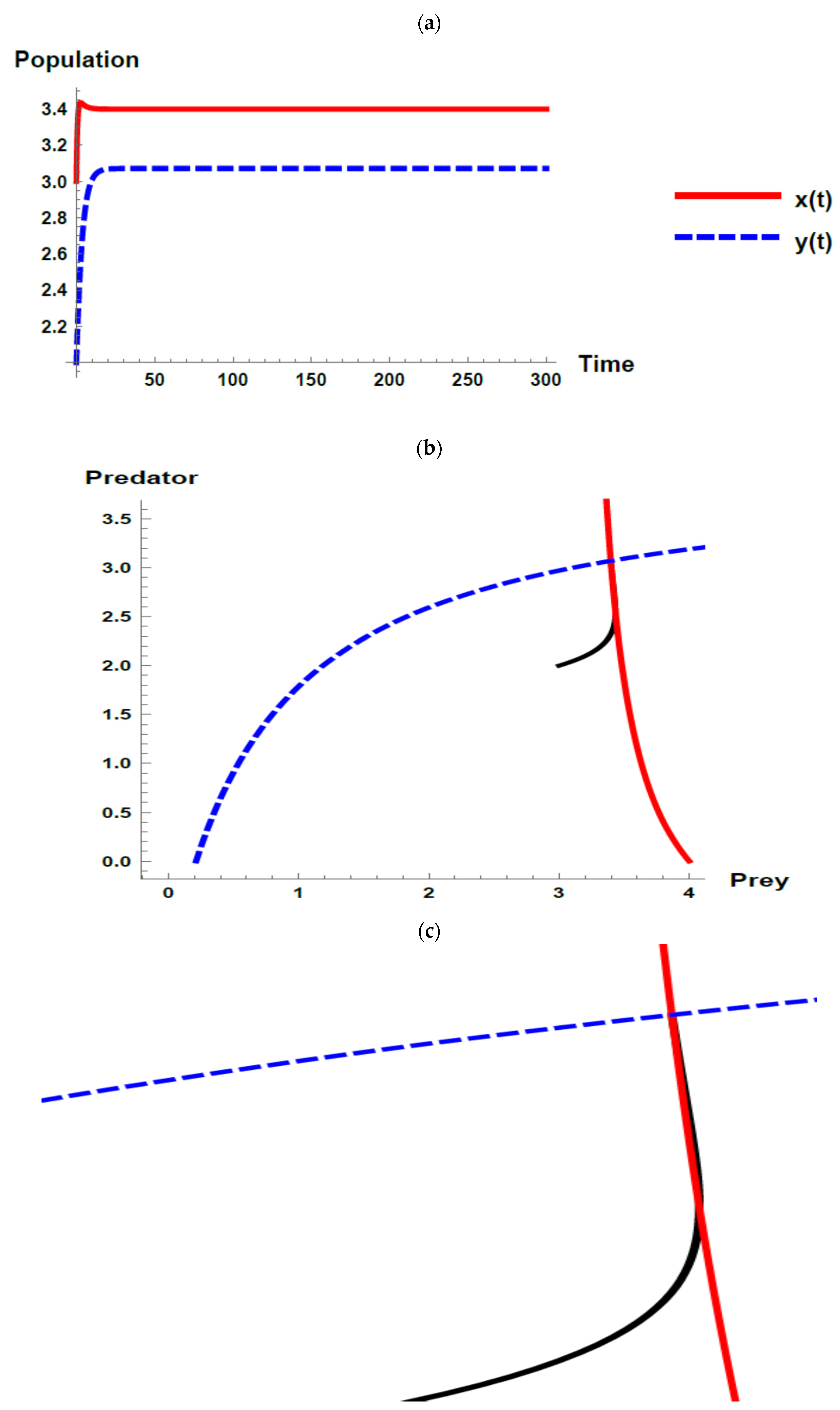
By using the first set of parameter values without considering the oscillation of the immigration of the prey, all the Kolmogorov conditions are satisfied. Thus, according to Proposition 2, the unique positive coexistence equilibrium point is ( 3.39753 ,   3.07037 ) . According to Theorem 4 and Theorem 6, it is locally and globally asymptotically stable since it satisfies condition (25), see Figure 1. Therefore, the dynamic behavior of the model (1) in the first set is steady state coexistence according to Proposition 2 and Theorem 6.
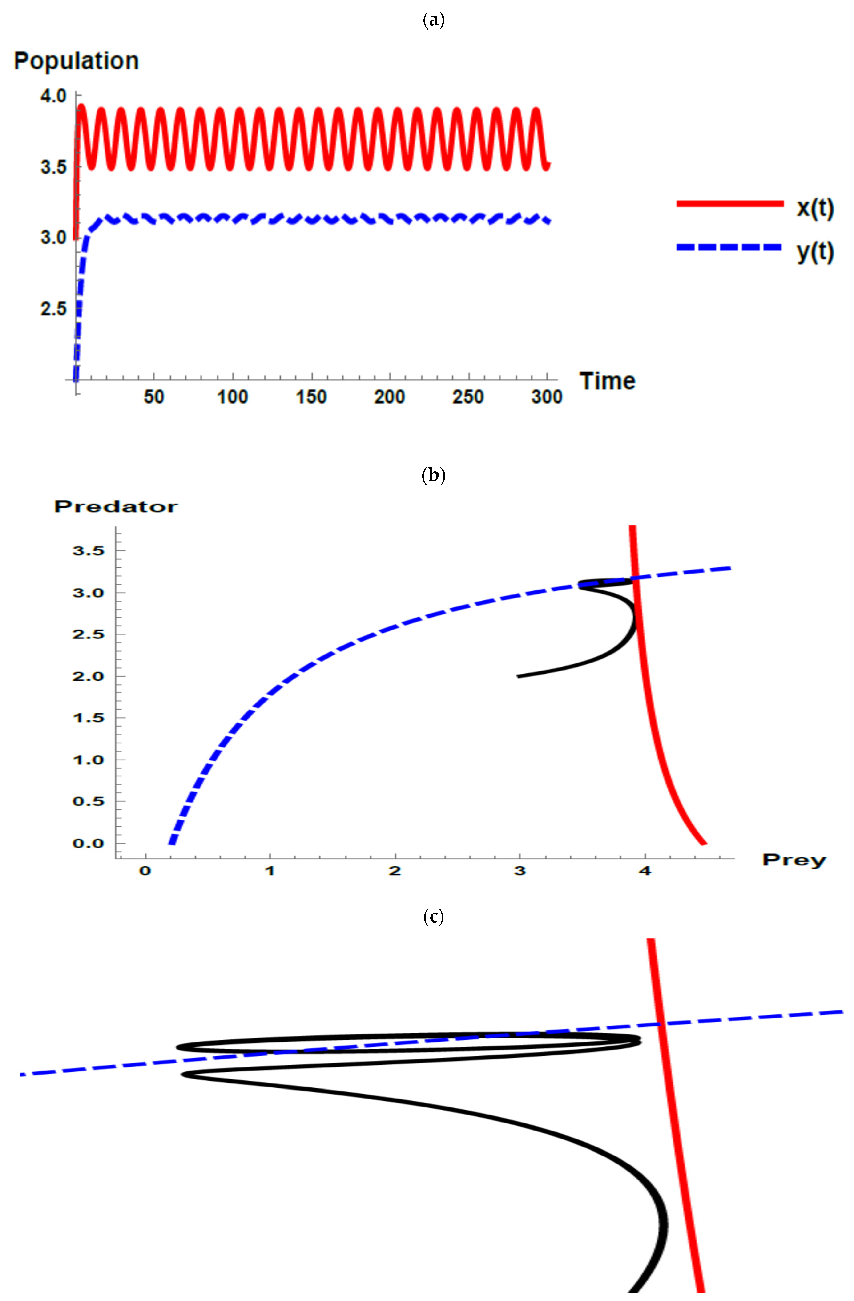
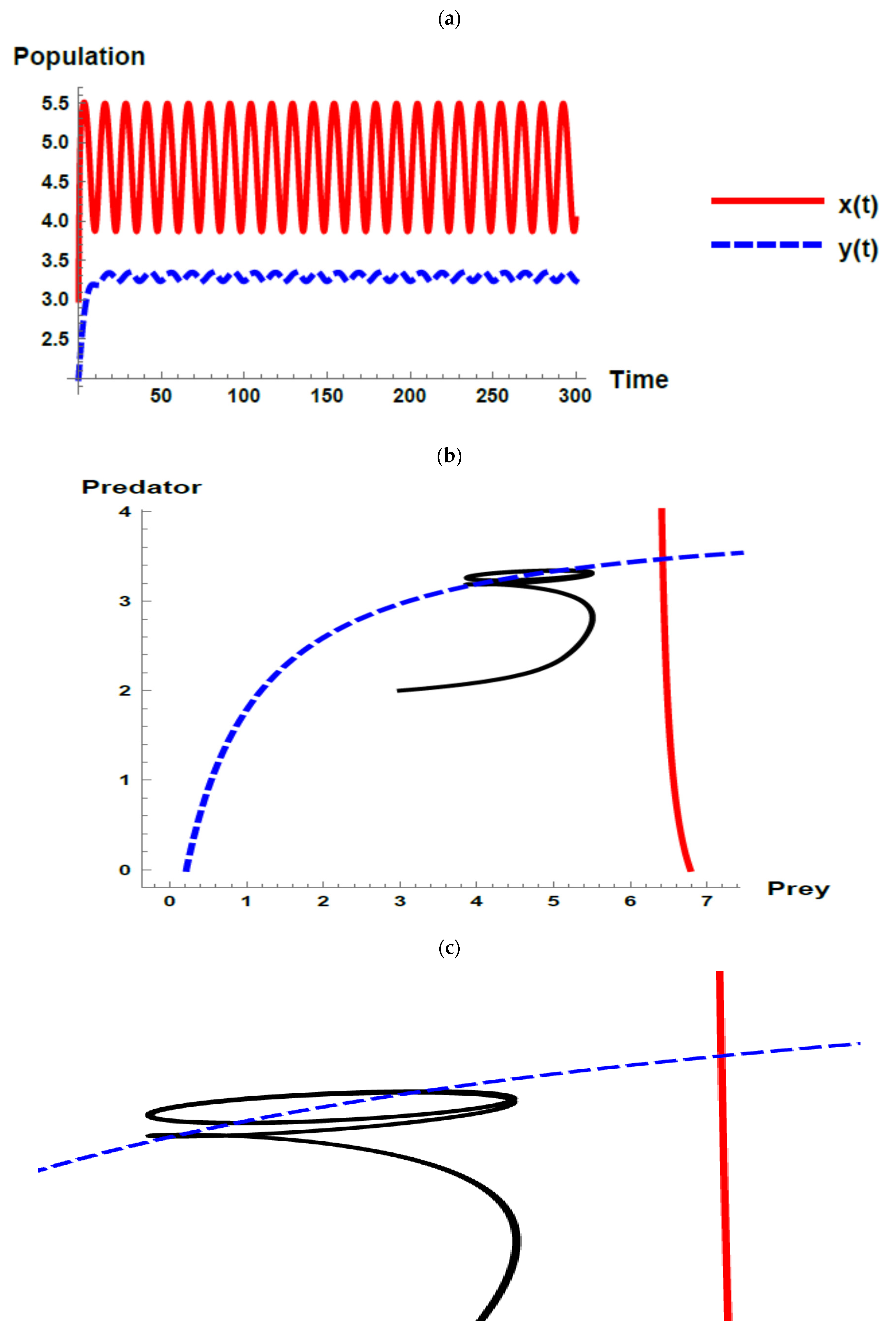
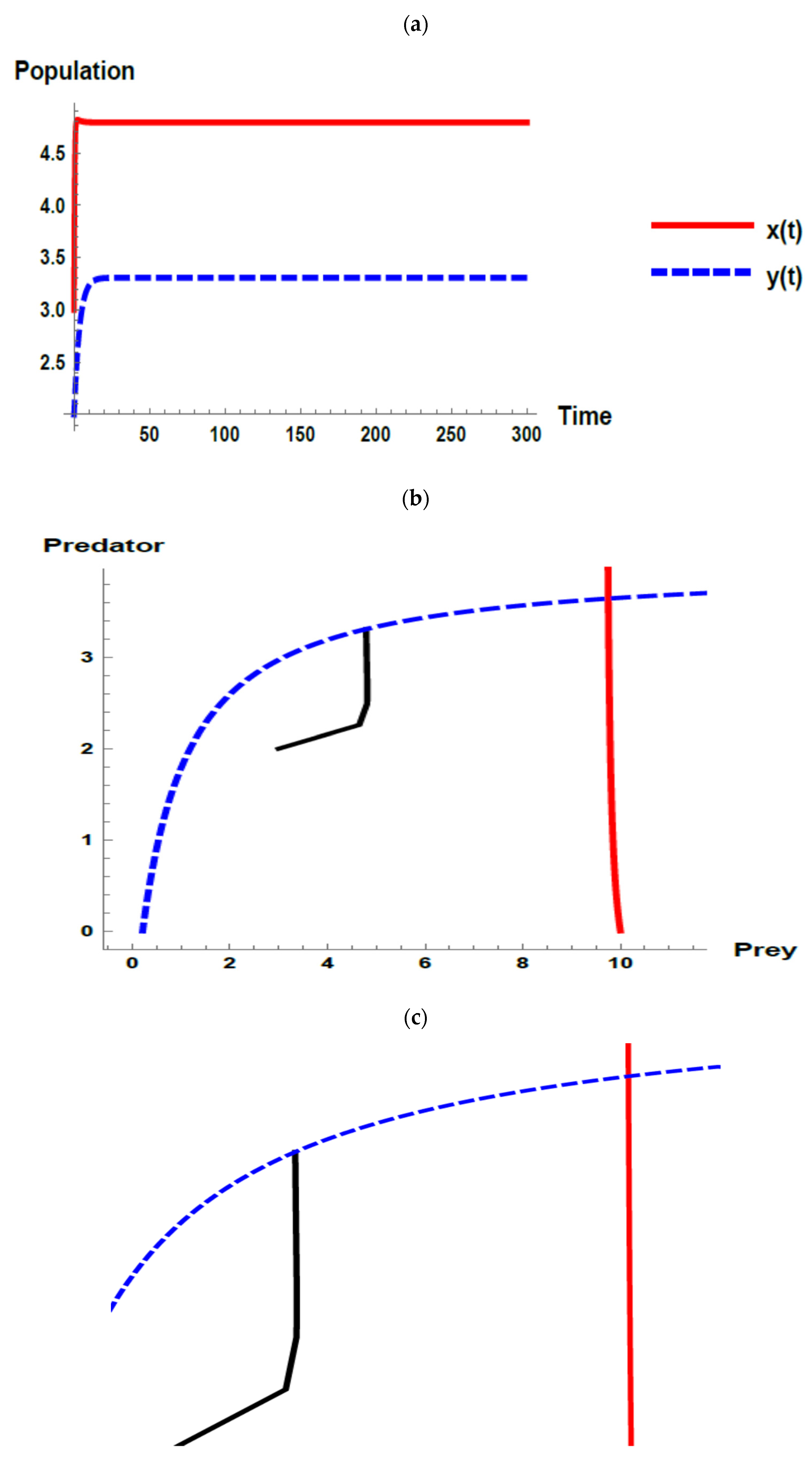
However, when investigating the oscillation of immigration of the prey, the dynamic behaviors of the model (32) tend to exhibit stable fluctuated and the fluctuations increase because of the increasing immigration parameter and the oscillation parameter that exists within the immigration, which is displayed through Figure 2, Figure 3 and Figure 4. On the other side, when the value of the immigration parameter ( i ) increases, the joint equilibrium point of predator and prey increases and moves away from the axes where the predator and prey isoclines cross as shown through Figure 2b, Figure 3b, Figure 4b and Figure 5b. It was interpreted that the likelihood of the coexistence of the predator–prey system increases as the value of i increases. Moreover, in the last case (i.e., i = 3.0 ), when neglecting the oscillation parameter i.e., ϵ = 0 , the likelihood of the coexistence of the predator–prey system increases more because the joint equilibrium point of the predator and prey increases and moves away from the axes where the predator and prey isoclines cross as displayed through Figure 5b, in addition, the densities of the prey and predator increase as shown in Figure 5a.
The second set of parameter values is considered as follows:
ζ = 1.4 ,   k = 3.0 ,   c = 11.00 ,   h = 2.85 ,   σ = 2.0 ,   μ = 0.9 ,   γ = 1.0 ,   ϵ = 0.75 ,   w = 0.5 .
Using the second set of parameter values without considering the oscillation in immigration, the dynamic behavior of model (1) is fluctuated coexistence, but close to axes, which increases the likelihood of extinction as depicted in Figure 6. This case corresponds with Proposition 1 and Corollary 2. In addition, all the Kolmogorov conditions are satisfied and the dynamic behavior stably fluctuates.
However, when investigating the oscillation of immigration, the dynamic behavior of the model (32) still fluctuated with the increasing immigration parameter and the oscillation parameter that exists within the immigration. Although the dynamic behavior is fluctuated, it moves away from the axes as shown through Figure 7b, Figure 8b, Figure 9b and Figure 10b, and it is interpreted that the likelihood of coexistence of the predator–prey system increases as the value of i increases. Moreover, in the last case (i.e., i = 3.0 ), when neglecting the oscillation parameter, i.e., ϵ = 0 , the likelihood of the coexistence of the system increases because the joint equilibrium point of the predator and prey increases and moves away from the axes where the predator and prey isoclines cross as displayed through Figure 10b, in addition, the densities of the prey and predator increase as shown in Figure 10a.
In Figure 9 and Figure 10, it was noticed that the dynamic of the system tends to exhibit more stably and coexist as shown through the Figure 9b or Figure 10b that present the changing shape of the predator isocline, which can be interpreted that the dynamic of the system is in state of disequilibrium when using the second set of parameter values, but when adding the oscillation of immigration of the prey into the system, makes the system tend to exhibit a more stable coexistence.

6. Discussion and Conclusions

In this study, one of the most preferable and complicated predator-dependent functional and numerical responses is investigated to form an autonomous predator–prey model. The functional and numerical responses are namely Crowley–Martin type. The Crowley–Martin type is preferable because it was developed based on the Holling type II, which is well documented in the literature. The main dynamic behaviors of model (1) are studied. The boundedness of the model (1) is proved in Theorem 1.
The Kolmogorov analysis is employed to endorse the predator–prey model (1) and to identify the coexistence and extinction conditions. Furthermore, the local stability was analyzed by using the Jacobian matrix. The eigenvalues were determined to obtain the local stability conditions. Furthermore, the global stability is proved by using a Lyapunov function and the Bendixson–Dulac criterion under the same local stability conditions.
The theoretical results of this study are explained as follows. Our model has three non-negative equilibrium points, which is biologically feasible. However, the coexistence equilibrium point is the most important point because it represents the predator–prey interaction. This exists under certain conditions, as explained through Proposition 1. The stability conditions are obtained for each equilibrium point, as explained in Theorems 2–6. Corollary 2 explains that the coexistence equilibrium point has periodic dynamics. The coexistence and extinction conditions are identified, as shown in Proposition 2 and Corollary 1.
The oscillation of immigration of the prey is investigated to form a non-autonomous model. To the best of our knowledge, this is the first study to investigate the oscillation of immigration in predator–prey models; this makes the model more effective and realistic due to the existence of real factors such as environmental and human factors that may cause a fluctuation of immigration. The numerical simulations were performed by taking two different sets of the hypothetical values of the parameters to represent two different dynamics that are steady state and fluctuated, respectively. The numerical results showed that there are new remarkable outcomes that can be summarized as follows:
When using the first set of parameter values, the following can be concluded:
  • Without consideration the oscillation of the immigration of the prey, the dynamic behavior of the system is in steady state coexistence. This coincides with the theoretical analysis of Proposition 2 and Theorem 6.
  • However, when investigating the oscillation of immigration of the prey, the dynamic behavior of the system tends to exhibit stable fluctuations which increase because of the increase in the immigration parameter and the oscillation parameter that exists within the immigration.
  • The likelihood of coexistence of the system increases as the value of immigration parameter increases. In addition to, when neglecting the oscillation parameter i.e., ϵ = 0 , the likelihood of coexistence of the system increases more.
When using the second set of parameter values, the following is concluded:
  • Without consideration the oscillation of immigration of the prey, the dynamic behavior of the system is in fluctuated coexistence. This coincides with the theoretical analysis in Proposition 1 and the Corollary.
  • However, when investigating the oscillation of the immigration of the prey, the dynamic behavior of the system tends to exhibit stable fluctuations which increase because of the increase in the immigration parameter and the oscillation parameter that exists within the immigration.
  • The likelihood of the coexistence of the system increases as the value of the immigration parameter increases. In addition, when neglecting the oscillation parameter, i.e., ϵ = 0 , the likelihood of coexistence of the system increases more.
  • The dynamic of the system tends to exhibit a more stable coexistence as the immigration parameter increases.
Some of the results of this study are consistent with previous findings on the effect of small immigration in a predator-prey system, where it demonstrates that the system stabilizes with adding positive immigration [26], as in the latter cases of the first and second sets in this study. However, the dynamic behaviors exhibit increasing fluctuations, but they display stable fluctuations and the coexistence of the system was paid more attention in this study, where the likelihood of the coexistence of the system increases as the value of the immigration parameter increases. In nature, there are some ecological interpretations may support the obtained outcomes in this study such as the rescue effect [41], which is a phenomenon explaining the increase in the likelihood of coexistence through immigration [42,43].

Funding

This paper received no external funding.

Data Availability Statement

Data is included within the article.

Acknowledgments

The author is highly grateful to the editors and the anonymous reviewers for their constructive comments that improved the presentation of this paper.

Conflicts of Interest

The author declares no conflict of interest.

References

  1. Hadeler, K.P.; Freedman, H.I. Predator-prey population with parasite infection. J. Math. Biol. 1989, 27, 609–631. [Google Scholar] [CrossRef] [PubMed]
  2. Kuang, Y.; Beretta, E. Global qualitative analysis of a ratio-dependent predator-prey system. J. Math. Biol. 1998, 36, 389–406. [Google Scholar] [CrossRef]
  3. Murray, J.D. Mathematical Biology; Springer: New York, NY, USA, 2002; Volume 2. [Google Scholar]
  4. Hsu, S.-B.; Hwang, T.-W.; Kuang, Y. A ratio-dependent food chain model and its applications to biological control. Math. Biosci. 2003, 181, 55–83. [Google Scholar] [CrossRef]
  5. Alebraheem, J.; Abu-Hassan, Y. Dynamics of a two predator-one prey system. Comput. Appl. Math. 2014, 33, 767–780. [Google Scholar] [CrossRef]
  6. Al-Moqbali, M.K.A.; Al-Salti, N.S.; Elmojtaba, I.M. Prey–Predator Models with Variable Carrying Capacity. Mathematics 2018, 6, 102. [Google Scholar] [CrossRef] [Green Version]
  7. Lotka, A.J. Elements of Physical Biology; Williams & Wilkins: Baltimore, MD, USA, 1925. [Google Scholar]
  8. Volterra, V. Variazione e fluttuazini del numero d’individui in specie animali conviventi. Mem R Accad. Naz Lincei 1926, 2, 31–113. [Google Scholar]
  9. Kuang, Y. Basic properties of mathematical population models. J. Biomath. 2002, 17, 129–142. [Google Scholar]
  10. Rockwood, L.L. Introduction to Population Ecology; Cambridge University Press: Cambridge, UK, 2006. [Google Scholar]
  11. Solomon, M.E. The natural control of animal populations. J. Anim. Ecol. 1949, 18, 1–35. [Google Scholar] [CrossRef]
  12. Holling, C.S. Some Characteristics of Simple Types of Predation and Parasitism. Can. Entomol. 1959, 91, 385–398. [Google Scholar] [CrossRef]
  13. Crowley, P.H.; Martin, E.K. Functional responses and interference within and between year classes of a dragonfly population. J. North. Am. Benth Soc. 1989, 8, 211–221. [Google Scholar] [CrossRef]
  14. Upadhyay, R.K.; Naj, R.K. Dynamics of a three species food chain model with Crowley-Martin type functional response. Chaos Solit. Fractals. 2009, 42, 1337–1346. [Google Scholar] [CrossRef]
  15. Ali, N.; Jazar, M. Global dynamics of a modified Leslie–Gower predator–prey model with Crowley–Martin functional responses. J. Appl. Math. Comput. 2013, 43, 271–293. [Google Scholar] [CrossRef]
  16. Shi, X.Y.; Zhou, X.Y.; Song, X.Y. Analysis of a stage-structured predator–prey model with Crowley–Martin function. J. Appl. Math. Comput. 2011, 36, 459–472. [Google Scholar] [CrossRef]
  17. Meng, X.Y.; Huo, H.F.; Xiang, H.; Yin, Q. Stability in a predator-prey model with Crowley-Martin function and stage structure for prey. Appl. Math. Comput. 2014, 232, 810–819. [Google Scholar] [CrossRef]
  18. Maiti, A.; Dubey, B.; Chakraborty, A. Global analysis of a delayed stage structure prey–predator model with Crowley–Martin type functional response. Math. Comput. Simul. 2019, 162, 58–84. [Google Scholar] [CrossRef]
  19. Alebraheem, J.; Abu-Hassan, Y. Simulation of complex dynamical behaviour in prey predator model. In Proceedings of the 2012 International Conference on Statistics in Science, Business and Engineering, Langkawi, Malaysia, 10–12 September 2012. [Google Scholar] [CrossRef]
  20. Mortoja Golam, S.K.; Panja, P.; Mondal, S.K. Dynamics of a predator-prey model with nonlinear incidence rate, Crowley-Martin type functional response and disease in prey population. Ecol. Gen. Genom. 2019, 10, 100035. [Google Scholar] [CrossRef]
  21. Ren, J.; Yu, L.; Siegmund, S. Bifurcations and chaos in a discrete predator-prey model with Crowley-Martin functional response. Nonlinear Dyn. 2017, 90, 19–41. [Google Scholar] [CrossRef]
  22. Liu, W.; Cai, D. Bifurcation, chaos analysis and control in a discrete-time predator–prey system. Adv. Differ. Equ. 2019, 2019, 11. [Google Scholar] [CrossRef]
  23. Liu, X.-Q.; Zhong, S.-M.; Tian, B.-D.; Zheng, F.-X. Asymptotic properties of a stochastic predator-prey model with Crowley-Martin functional response. Appl. Math. Comput. 2013, 43, 479–490. [Google Scholar] [CrossRef]
  24. Xu, C.; Ren, G.; Yu, Y. Extinction Analysis of Stochastic Predator–Prey System with Stage Structure and Crowley–Martin Functional Response. Entropy 2019, 21, 252. [Google Scholar] [CrossRef] [Green Version]
  25. Mukherjee, D. The effect of refuge and immigration in a predator–prey system in the presence of a competitor for the prey. Nonlinear Anal. Real World Appl. 2016, 31, 277–287. [Google Scholar] [CrossRef]
  26. Tahara, T.; Gavina, M.K.A.; Kawano, T.; Tubay, J.M.; Rabajante, J.F.; Ito, H.; Morita, S.; Ichinos, G.; Okabe, T.; Togashi, T.; et al. Asymptotic stability of a modified Lotka-Volterra model with small immigrations. Sci. Rep. 2018, 8, 7029. [Google Scholar] [CrossRef] [PubMed]
  27. Upadhyay, R.K.; Iyengar, S. Effect of seasonality on the dynamics of 2and 3 species prey-predator systems. Nonlinear Anal. Real World Appl. 2007, 6, 509–530. [Google Scholar] [CrossRef]
  28. Gakkhar, S.; Naji, R.K. Seasonally perturbed prey-predator system with predator-dependent functional response. Chaos Solitons Fractals 2003, 18, 1075–1083. [Google Scholar] [CrossRef]
  29. Alebraheem, J. Fluctuations in interactions of prey predator systems. Sci. Int. 2016, 28, 2357–2362. [Google Scholar]
  30. Freedman, I. Deterministic Mathematical Models in Population Ecology; Marcel Dekker, Inc.: New York, NY, USA, 1980. [Google Scholar]
  31. Sigmund, K. Kolmogorov and Population Dynamics, Kolmogorovs Heritage in Mathematics; Springer: Berlin/Heidelberg, Germany, 2007; pp. 177–186. [Google Scholar]
  32. Dubey, B.; Upadhyay, R. Persistence and extinction of one-prey and two-predator system. Nonlinear Anal. 2004, 9, 307–329. [Google Scholar] [CrossRef]
  33. Huo, H.F.; Ma, Z.P.; Liu, C.Y. Persistence and stability for a generalized leslie-gower model with stage structure and dispersal. Abstr. Appl. Anal. 2009, 2009, 135843. [Google Scholar] [CrossRef]
  34. Kar, T.; Batabyal, A. Persistence and stability of a two prey one predator system. Int. J. Eng. Sci. Technol. 2010, 2, 174–190. [Google Scholar] [CrossRef]
  35. Tian, X.; Xu, R. Global dynamics of a predator-prey system with holling type II functional response. Nonlinear Anal. Model. Control. 2011, 16, 242–253. [Google Scholar] [CrossRef] [Green Version]
  36. Alebraheem, J.; Abu-Hasan, Y. The Effects of Capture Efficiency on the Coexistence of a Predator in a Two Predators-One Prey Model. J. Appl. Sci. 2011, 11, 3717–3724. [Google Scholar] [CrossRef]
  37. Alebraheem, J.; Abu-Hasan, Y. Persistence of Predators in a Two Predators-One Prey Model with Non-Periodic Solution. Appl. Math. Sci. 2012, 6, 943–956. [Google Scholar]
  38. Alebraheem, J. Relationship between the Paradox of Enrichment and the Dynamics of Persistence and Extinction in Prey-Predator Systems. Symmetry 2018, 10, 532. [Google Scholar] [CrossRef] [Green Version]
  39. Tunç, C.; Tunç, O. Qualitative analysis for a variable delay system of differential equations of second order. J. Taibah Univ. Sci. 2019, 13, 468–477. [Google Scholar] [CrossRef] [Green Version]
  40. Shah, K.; Tunç, C. Existence theory and stability analysis to a system of boundary value problem. J. Taibah Univ. Sci. 2017, 11, 1330–1342. [Google Scholar] [CrossRef] [Green Version]
  41. Brown, J.H.; Kodric-Brown, A. Turnover rates in insular biogeography: Effect of immigration on extinction. Ecology 1977, 58, 445–449. [Google Scholar] [CrossRef] [Green Version]
  42. Richards, C.M. Inbreeding depression and genetic rescue in a plant metapopulation. Am. Nat. 2000, 155, 383–394. [Google Scholar] [CrossRef] [PubMed]
  43. Eriksson, A.; Elías-Wolff, F.; Mehlig, B.; Manica, A. The emergence of the rescue effect from explicit within-and between-patch dynamics in a metapopulation. Proc. R. Soc. B 2014, 281, 20133127. [Google Scholar] [CrossRef] [Green Version]
Figure 1. Dynamic behavior of the first set when ( i = 0.0 ): (a) time series; (b) zero-growth isoclines of the prey ( Diversity 13 00023 i001) and predator ( Diversity 13 00023 i002) populations and phase plane trajectories; (c) cross-sectional picture of (b).
Diversity 13 00023 g001
Figure 2. Dynamic behavior of the first set when ( i = 0.1 ): (a) time series; (b) zero-growth isoclines of the prey ( Diversity 13 00023 i001) and predator ( Diversity 13 00023 i002) populations and phase plane trajectories; (c) cross-sectional picture of (b).
Diversity 13 00023 g002
Figure 3. Dynamic behavior of the first set when ( i = 0.5 ): (a) time series; (b) zero-growth isoclines of the prey ( Diversity 13 00023 i001) and predator ( Diversity 13 00023 i002) populations and phase plane trajectories; (c) cross-sectional picture of (b).
Diversity 13 00023 g003
Figure 4. Dynamic behavior of the first set when ( i = 3.0 ): (a) time series; (b) zero-growth isoclines of the prey ( Diversity 13 00023 i001) and predator ( Diversity 13 00023 i002) populations and phase plane trajectories; (c) cross-sectional picture of (b).
Diversity 13 00023 g004
Figure 5. Dynamic behavior of the first set when ( i = 3.0 ,   ϵ = 0 ): (a) time series; (b) zero-growth isoclines of the prey ( Diversity 13 00023 i001) and predator ( Diversity 13 00023 i002) populations and phase plane trajectories; (c) cross-sectional picture of (b).
Diversity 13 00023 g005
Figure 6. Dynamic behavior of the second set when ( i = 0.0 ): (a) time series; (b) zero-growth isoclines of the prey ( Diversity 13 00023 i001) and predator ( Diversity 13 00023 i002) populations and phase plane trajectories; (c) cross-sectional picture of (b).
Diversity 13 00023 g006
Figure 7. Dynamic behavior of the second set when ( i = 0.1 ): (a) time series; (b) zero-growth isoclines of the prey ( Diversity 13 00023 i001) and predator ( Diversity 13 00023 i002) populations and phase plane trajectories; (c) cross-sectional picture of (b).
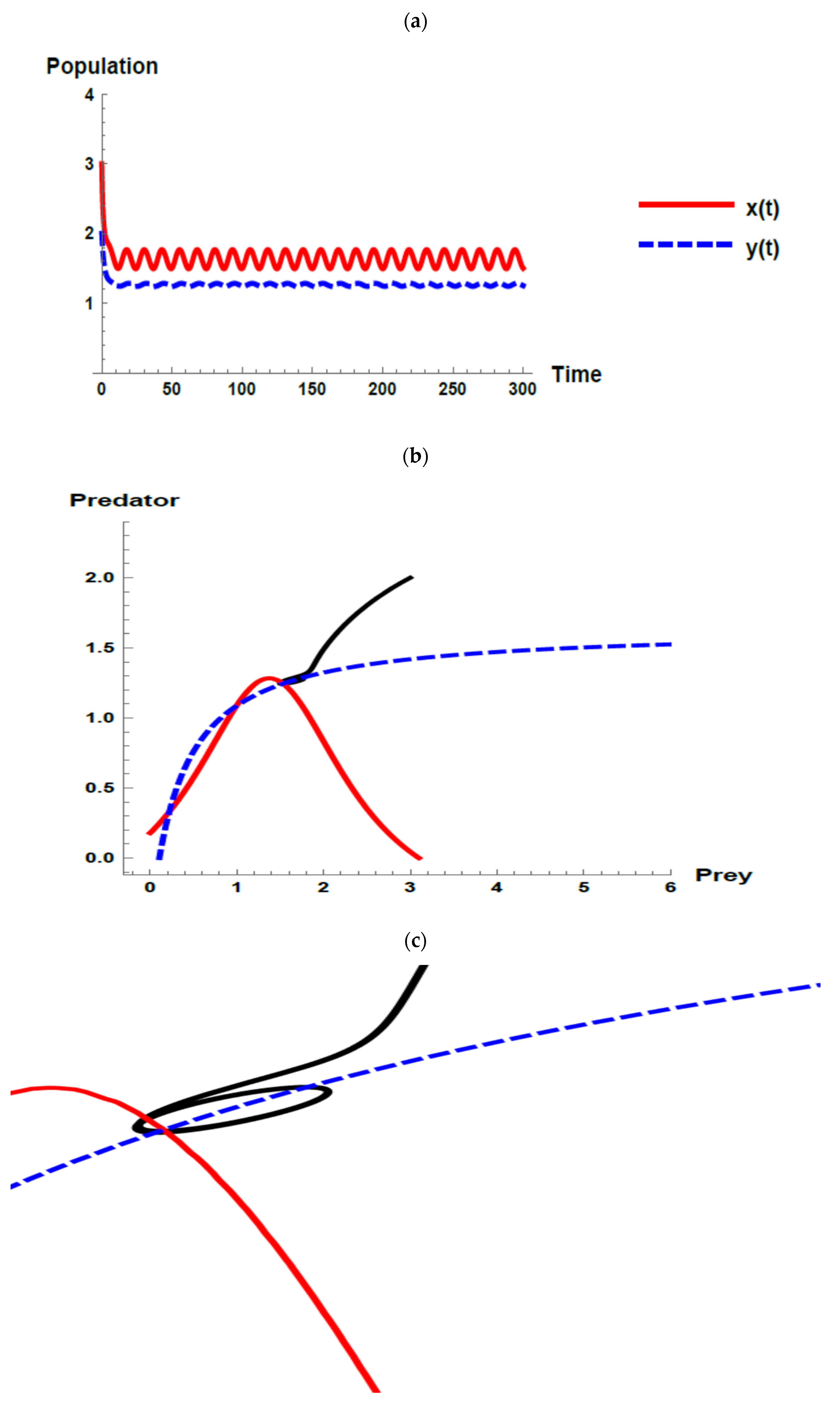
Diversity 13 00023 g007
Figure 8. Dynamic behavior of the second set when ( i = 0.5 ): (a) time series; (b) zero-growth isoclines of the prey ( Diversity 13 00023 i001) and predator ( Diversity 13 00023 i002) populations and phase plane trajectories; (c) cross-sectional picture of (b).
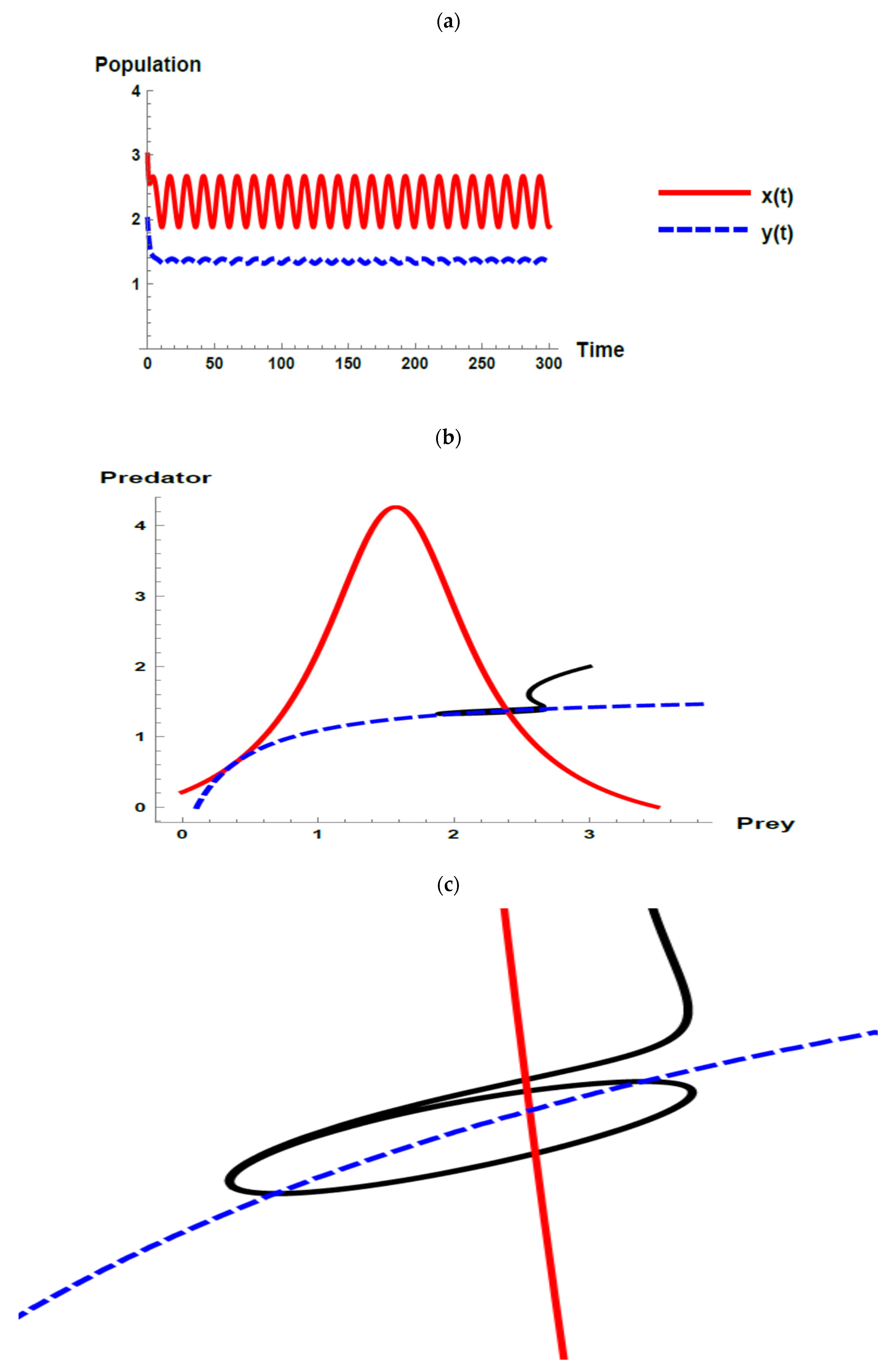
Diversity 13 00023 g008
Figure 9. Dynamic behavior of the second set when ( i = 3.0 ): (a) time series; (b) zero-growth isoclines of the prey ( Diversity 13 00023 i001) and predator ( Diversity 13 00023 i002) populations and phase plane trajectories; (c) cross-sectional picture of (b).
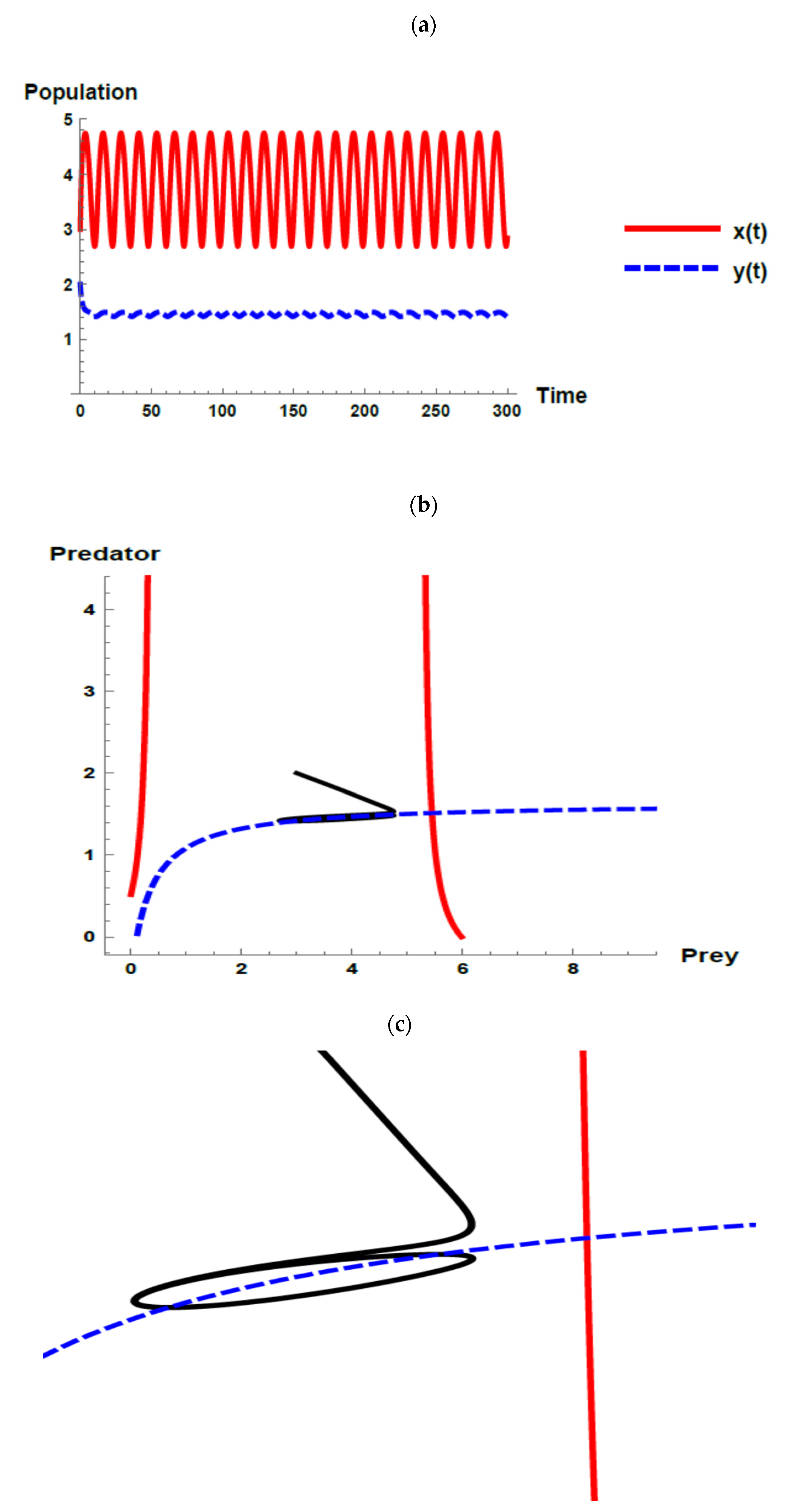
Diversity 13 00023 g009
Figure 10. Dynamic behavior of the second set when ( i = 3.0 ,   ϵ = 0 ): (a) time series; (b) zero- growth isoclines of the prey ( Diversity 13 00023 i001) and predator ( Diversity 13 00023 i002) populations and phase plane trajectories; (c) cross-sectional picture of (b).
Diversity 13 00023 g010
Publisher’s Note: MDPI stays neutral with regard to jurisdictional claims in published maps and institutional affiliations.