Article

A Trait-Based Clustering for Phytoplankton Biomass Modeling and Prediction

by
Crispin M. Mutshinda
1,*,
Zoe V. Finkel
2,
Claire E. Widdicombe
3 and
Andrew J. Irwin
1
1
Department of Mathematics and Statistics, Dalhousie University, Halifax, NS B3H 4R2, Canada
2
Department of Oceanography, Dalhousie University, Halifax, NS B3H 4R2, Canada
3
Plymouth Marine Laboratory, Prospect Place, Plymouth PL1 3DH, UK
*
Author to whom correspondence should be addressed.
Diversity 2020, 12(8), 295; https://doi.org/10.3390/d12080295
Submission received: 8 June 2020 / Revised: 20 July 2020 / Accepted: 21 July 2020 / Published: 28 July 2020

Abstract

:
When designing models for predicting phytoplankton biomass or characterizing traits, it is useful to aggregate the myriad of species into a few biologically meaningful groups and focus on group-level attributes, the common practice being to combine phytoplankton species by functional types. However, biogeochemists and plankton ecologists debate the most applicable grouping for describing phytoplankton biomass patterns and predicting future community structure. Although trait-based approaches are increasingly being advocated, methods are missing for the generation of trait-based taxa as alternatives to functional types. Here we introduce such a method and demonstrate the usefulness of the resulting clustering with field data. We parameterize a Bayesian model of biomass dynamics and analyze long-term phytoplankton data collected at Station L4 in the Western English Channel between April 2003 and December 2009. We examine the tradeoffs encountered regarding trait characterization and biomass prediction when aggregating biomass by (1) functional types, (2) the trait-based clusters generated by our method, and (3) total biomass. The model conveniently extracted trait values under the trait-based clustering, but required well-constrained priors under the functional type categorization. It also more accurately predicted total biomass under the trait-based clustering and the total biomass aggregation with comparable root mean squared prediction errors, which were roughly five-fold lower than under the functional type grouping. Although the total biomass grouping ignores taxonomic differences in phytoplankton traits, it predicts total biomass change as well as the trait-based clustering. Our results corroborate the value of trait-based approaches in investigating the mechanisms underlying phytoplankton biomass dynamics and predicting the community response to environmental changes.

Graphical Abstract

1. Introduction

Phytoplankton communities are extremely diverse, with typically several thousands of species [1]. When developing models to project biomass or characterize traits, it is convenient to aggregate species into a few biologically meaningful groups and focus on group-level characteristics [2,3,4,5]. This greatly simplifies the model parameterization since it is much easier to deal with a few taxa than the multitude of individual species. The collection of the myriad of species to a handful of taxa is important statistically as well, particularly when many species are frequently missing or at abundances below common detection limits raising missing data issues, let alone the fact that predicting the pooled biomass of many species is easier than predicting the biomass of each individual species.
The usual practice is to aggregate phytoplankton species by functional types based on ecological functions or biogeochemical roles [6,7,8,9]. While functional types are sensible proxies for biogeochemical functions, several studies [8,10,11,12] have emphasized that functionally similar species may greatly differ in traits that govern their biomass dynamics. Moreover, biogeochemists and plankton ecologists often debate the most appropriate grouping for describing the biomass patterns of phytoplankton assemblages and predicting future community structure [13]. Nonetheless, trait-based approaches are increasingly advocated as valuable for synthesizing data across species [8,14,15,16,17,18,19,20]. Trait-based approaches shift the focus from species identities to trait values, on the premise that community structure results essentially from tradeoffs between important traits. There is often a confusion about the meaning of the term “trait”. Following [15], we consider as trait any characteristic impacting fitness either directly or via its effect on growth, reproduction and survival (the three components of individual performance). Accordingly, body size, maximum growth rate in resource-replete conditions, and half-saturation constants for limiting resources are traits. The traits used in phytoplankton models vary widely depending of the question of interest, but commonly include the maximum growth rate under resource-replete conditions, light and nutrient acquisition and use, predator avoidance, and temperature sensitivity [8]. While traits have a clear meaning for species, it is not always obvious what they mean biologically for groups of species such as functional types. However, we need some way of aggregating species to simplify the biomass dynamics model. Generally, characteristics of the cells that determine whether a species (or group of species) does well under specific conditions are traits. The application of the trait concept to a group of species rather than single species is a somewhat unusual feature of our analysis, but this approach is common in biogeochemical modeling literature [21]. Although trait-based approaches are increasingly suggested, techniques for generating trait-based groupings are missing.
In this study, we introduce a method for generating a trait-based clustering of phytoplankton as an alternative to the prevalent functional type categorization. Our primary interest is in estimating trait values and predicting total biomass from a time series of species-level biomass records and environmental data. Species-level abundance and biomass data often include missing values which are either due to actual absences or to the fact that many species frequently occur at abundances below common detection thresholds. To avoid missing data issues, our method initially relies on occurrence data and proceeds in two steps. The first involves analyzing the environmental controls of the presence-absence of individual species and summarizing these controls in trait values. The second generates a trait-based grouping by building a clustering on top of the occurrence trait values. Because estimates may be uncertain for some of the occurrence traits, a principal component analysis (PCA) is used to determine the directions of maximum variation in occurrence trait values. Species scores on the leading principal components of occurrence traits are then used as features for the trait-based clustering. The Gaussian mixture model (GMM) is a soft clustering method, meaning that each species can belong to multiple clusters with different probabilities, called cluster responsibilities or cluster assignment probabilities, summing to one. In contrast, hard clustering methods such as the k-means algorithm assign each instance to a single cluster exclusively. We use the soft-clustering approach of GMM since we anticipate that some species may share traits with species in more than one cluster. For the purpose of biomass dynamics analysis, we compute the biomass time series of each cluster by combining the biomass time series of individual species with the cluster assignment probabilities so that at any time over the study period, each species contributes biomass to all clusters in proportion to their respective responsibilities for that species. We illustrate the methodology with long-term species-level phytoplankton time series and coincident measurements of potentially important environmental variables describing water conditions and resource availability. We parameterize a Bayesian model of biomass dynamics and examine the tradeoffs encountered in connection with trait value characterization and biomass prediction when aggregating biomass according to (1) the functional types, (2) the trait-based clusters generated by our method, and (3) the total biomass (a single cluster). The group-level traits that we are interested in characterizing include the maximum growth rate, temperature and salinity sensitivity, and half-saturation constants for irradiance, nitrogen and silicate representing resource acquisition ability.

2. Materials and Methods

2.1. Description of Data

We consider a long-term series of weekly phytoplankton records for 74 species (57 diatoms and 17 dinoflagellates), along with coincident measurements of potentially important environmental variables recorded at Station L4 (50°15.00′ N, 4°13.02′ W) over 349 consecutive weeks between 14 April 2003 and 21 December 2009. Station L4 is located in the Western English Channel about 10 nautical miles south-west of Plymouth, UK, with a water column depth of approximately 50 m (Harris 2010). Phytoplankton samples were analyzed by microscopy [22] and converted to biomass using appropriate conversion factors based on empirically established carbon to volume relationships [23]. The environmental variables under consideration include sea-surface temperature (°C), photosynthetically active radiation (PAR; mol   m 2   d 1 ), salinity, and concentration ( μ mol   L 1 ) of dissolved inorganic nitrogen (nitrate + nitrite), silicate, and phosphate (Figure 1).
Before explaining the details of our proposed trait-based clustering procedure and illustrating the value of the ensuing clustering with the L4 data, we start by specifying the Bayesian model describing the biomass dynamics of phytoplankton taxa. The structure of the biomass dynamics model is the same for all three clustering schemes examined in this study and can be used with any clustering of species.

2.2. Bayesian Model of Cluster-Level Biomass Dynamics

We model the biomass dynamics of a cluster of phytoplankton species by assuming that the realized growth rate is determined by cluster-specific traits governing the effect of environmental conditions (temperature, salinity) and resource availability (light and nutrients). Let Y g , w and Z k , w denote the biomass of cluster g and the Z-score (a standardized value indicating how many standard deviations an observation is above or below the mean), respectively, of the kth environmental condition (temperature and salinity) during week w . We assume that Y g , w depends on Y g , w 1 and on the set of abiotic factors under consideration as:
Y g , w = Y g , w 1   exp ( μ g , w + k = 1 2 β g , k   Z k , w )   η g , w
where μ g , w is the realized net growth rate of taxon g from week w 1 to w at average environmental conditions, β g , k is the effect of the kth environmental condition on biomass growth for cluster g , and η g , w ( w = 1 , , W ) are multiplicative noise terms assumed to be log-normality distributed and serially independent. The log-normality assumption on the biomass distribution is sensible on theoretical and empirical grounds [8,24]. For purposes of estimating the model parameters, it is convenient to re-write Equation (1) on the natural logarithmic scale. That is,
y g , w = y g , w 1 + μ g , w + k = 1 2 β g , k   Z k , w + ε g , w
where y g , w = ln ( Y g , w ) and ε g , w = ln ( η g , w ) . Biotic interactions and resource limitation enter the growth dynamics model by letting
μ g , w = r g ( 1 + h = 1 G α g h   ln ( Y h , w 1 ) k g )   L ( w , g )
where r g is the intrinsic rate of biomass growth for cluster g representing the maximum net growth rate of that cluster at average environmental conditions and no resource limitation. The parameter α g , h represents the effect of cluster h on the growth of cluster g , with all intra-specific effects α g , g set equal to −1 [25,26], k g is the carrying capacity of cluster g intended to capture density-dependent feedbacks. Finally, P A R w , N i t w and S i l w denote respectively photosynthetic active radiation, nitrogen concentration and silicate concentration during week w . Resource limitation to the growth rate of cluster g is captured by L ( w , g ) , which is a function of the resources available during week w , with 0 < L ( w , g ) 1 . We assume that:
L ( w , g ) = min   { P A R w K E g + P A R w ,   N i t w K N g + N i t w ,   S i l w K S g + S i l w }
where K E g , K N g and K S g denote respectively the irradiance, nitrogen and silicate half-saturation constants for cluster g . The modeling of resource limitation by combining Michaelis–Menten saturating functions of various resources with the minimum function guarantees that the growth rate of each cluster is, at any time, solely limited by the scarcest resource (the resource with the lowest Michaelis–Menten term), in line with Liebig’s law of the minimum [27,28].

2.3. Description of the Trait-Based Clustering Method

Species-level abundance and biomass data for highly diverse systems such as plankton assemblages typically include missing values. To avoid missing data issues, our trait-based clustering methodology relies initially on presence-absence data, and proceeds in two steps as described in Section 2.3.1 and Section 2.3.2

2.3.1. Analyzing the Environmental Drivers of Species Occurrence

Let d s , t ( s = 1 , ,   N ,   t = 1 , , T ) represent the binary indicator for the presence of species s at time t so that d s , t = 1 when species s is observed at time t and d s , t = 0 otherwise, and let x j t ( j = 1 , , J ) indicate the Z -score of the jth environmental variable (temperature, salinity, irradiance, nitrogen, phosphate and silicate concentration) at time t . We assume that:
d s , t   ~ B e r n o u l l i ( π s , t )
where logit ( π s , t ) = π s , t / ( 1 π s , t ) depends linearly on the Z-scores of the abiotic variables at time t through:
logit ( π s , t ) = α s + j = 1 J β s , j   x j , t
In Equation (6), α s is the intercept specific to species s , β s , j is the regression coefficient of the jth variable for species s . In the Bayesian framework [29,30] adopted here, the logistic regression model is easy to fit by Markov chain Monte Carlo (MCMC) simulation [31] through freely available Bayesian software packages such as OpenBUGS [32]. The BUGS code for the logistic model is relatively easy to write (e.g., [33]).
The posterior estimates of the environmental effects for the occurrence model (herein occurrence traits) are potential features for our clustering procedure. Since some estimates may be very uncertain, we apply a principal component analysis (PCA) to the N × J matrix of species-specific occurrence trait value estimates (posterior means scaled by corresponding posterior standard deviations) to identify the directions of maximum variability (the leading principal components). PCA transforms a set of J correlated variables into a smaller number Q < J of new variables called principal components (PCs) or orthogonal components that are uncorrelated linear combinations of the initial variables retaining most of the variation. The first PC represents the direction of highest variability in the data; the second PC represents the direction of second highest variability in the data, and so on. Species scores on the leading PCs provide features for the clustering carried out in second step.

2.3.2. Clustering Using GMM and the E-M Algorithm

The clustering step is achieved by fitting a Gaussian mixture model (GMM) to species scores on the leading principal components of occurrence traits. The GMM is a convex linear combination of a finite number of Gaussians. For a d -dimensional feature space, the density of a point x d under a G -component GMM is given by:
p ( x ) = g = 1 G λ g N d ( x |   μ g , Σ g )
where λ g 0 is the mixing coefficient for the g th Gaussian ( g = 1 , , G ) with g   λ g = 1 . N d ( . | μ g , Σ g ) denotes the d-dimensional normal distribution with mean vector μ g d and covariance matrix Σ g d × d , and G is a pre-set number of mixture components. Although the GMM is a flexible model, it may involve a large number of parameters to estimate with no closed-form expression available when class memberships are unknown. A general technique for finding maximum likelihood estimators in models involving missing or latent variables is the expectation-maximization (EM) algorithm introduced in a general form by Dempster et al. [34]. The EM algorithm starts with an initial guess of the model parameters and alternates iteratively, until convergence, between the expectation (E) step that creates a function for the expectation of the log-likelihood evaluated at the current parameter values and the maximization (M) step that maximizes the expected log-likelihood obtained in the E step to re-estimate the parameters. The EM algorithm for fitting a G-component GMM starts with an initial guess of the model parameters namely, mean vectors { μ g } g = 1 G and the covariance matrices { Σ g } g = 1 G for each Gaussian, as well as a G-vector λ = ( λ 1 , , λ G ) of non-negative mixing weights summing to one. It then cycles iteratively until convergence between the E-step and the M-step described below.
E-step: determine for each species s ( s = 1 , N ) and each component g of the Gaussian mixture ( g = 1 , G ), the, the assignment score q s , g of species s to the g -th mixture component called the “responsibility” of the g th Gaussian mixture component for the feature vector x s d characterizing species s . This assignment score is computed as:
q s , g = Pr ( Cluster = g | x s ) = λ g   N d ( x s |   μ g , Σ g ) r = 1 G λ r   N d ( x s |   μ r , Σ r )
It is clear from Equation (8) that q s , g represents the relative density of x s under the g th Gaussian component. If x s is very likely under the g th Gaussian, q s , g will be large, and vice-versa. The denominator r = 1 G λ r   N d ( x s |   μ r , Σ r ) in Equation (8) is nothing but a normalizing factor guaranteeing that g = 1 G q s , g = 1 . The total responsibility allocated to the g th cluster
n g = s q s , g
represents the relative number of species assigned to the g th cluster, and g = 1 G n g = N is the total number of species under consideration.
M-step: update the parameters of each mixture component namely, the mean vector μ g and the covariance matrix Σ g ( g = 1 , , G ) as the weighted mean and weighted covariance matrix of the assigned data respectively, where the weights are given by the responsibilities obtained in the E-step. More specifically, compute:
μ g = 1 n g   s q s , g x s
Σ g = 1 n g   s q s , g   ( x s μ g ) ( x s μ g ) T    
The updated total responsibility allocated to cluster g determines the updated mixing coefficient λ g of cluster g through:
λ g = n g N
The model’s log-likelihood function is:
log p ( x ) = s log ( g = 1 G λ g   N d ( x s |   μ g , Σ g ) )
Since each iteration of the EM algorithm increases the log-likelihood [35], a plot of the observed data log-likelihood against the EM iteration number can indicate that the model has converged when the log-likelihood reaches a plateau and does not increase any further. Since the Gaussian mixture is a proper probability distribution, we can use the log-likelihood of the validation or the test set to assess the model fit. We can also determine the number of Gaussian components by maximizing the log-likelihood with respect to the number of clusters, starting with a single cluster.
For biomass dynamics modeling, we require the biomass time series of each cluster. Since the GMM produces a soft clustering, each species may contribute biomass to all clusters, in contrast to hard clustering procedures such as the k -means algorithm that assign each species to a single cluster exclusively. If B s , w and q s , g denote respectively the biomass of species s during week w and the responsibility of cluster g for species s , then the biomass contributed to cluster g by species s during week w is B s , w q s , g . Accordingly, the biomass Y g , w of cluster g during week w is given by:
Y g , w = s = 1 N B s , w q s , g
where N denotes the total number of species under consideration.

2.4. Application to the Station L4 Data

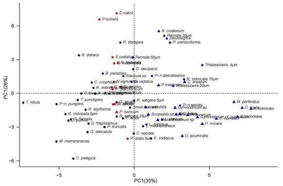
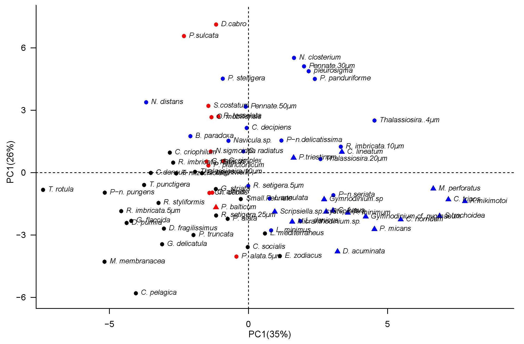
2.4.1. Analyzing the Environmental Controls of Species Occurrence

We first analyzed the factors that determine the presence-absence of individual species through the Bayesian logistic regression model described in Section 2.3, using sea-surface temperature, photosynthetically active radiation, salinity, nitrogen (nitrate + nitrite), silicate, and phosphate as environmental predictors. MCMC implemented in OpenBUGS allowed us to simulate from the joint posterior of the model parameters, yielding a good estimate of the joint posterior distribution of the model parameters from 16,000 iterations of three parallel Markov chains after discarding the first 6000 iterations of each Markov chain as burn-in period and thinning the remainder by a factor of 20.
Temperature and irradiance emerged as the key drivers of species occurrence patterns, followed by nitrogen. The temperature and irradiance responses were broadly negative for diatoms and positive for dinoflagellates, whereas nitrogen effects were largely positive for diatoms and negative for dinoflagellates. These results imply increased presence of diatoms at temperature and irradiance levels below the average values over the time series and higher than average nitrogen concentrations, in contrast with the dinoflagellates thriving in warm and nutrient-poor waters. These results are consistent with trends of taxonomic succession at Station L4 [22] and findings of previous analyses of the L4 data, including [8].
The first three principal components explained 76% of variation in occurrence trait values across species. Temperature and irradiance loadings dominated the first principal component accounting for 35% of variation, whereas nitrogen and phosphate loadings dominated the second and third principal components explaining 26% and 15% of total variation, respectively (Table 1).

2.4.2. Implementation of the Trait-Based Clustering

We generated our trait-based clustering by building a three-component GMM on top of species scores on the first three principal components of occurrence trait values. We used the EM algorithm implemented in R [36] through the mixtools package [37] to find maximum likelihood estimates of the GMM parameters. After roughly 15 EM iterations, the log-likelihood function reached a plateau, indicating convergence (Figure S1 in Supplementary Material). If for visualization purposes we consider the maximum a posteriori (MAP) clustering solution assigning each species s to the cluster with highest responsibility for its feature vector x s , the resulting clustering exhibits the following three striking features. (1) One of the clusters, Cluster 1, the second largest with twenty-six species, comprises exclusively diatoms. (2) All dinoflagellates except Prorocentrum balticum fall in the same cluster namely, Cluster 3, the largest cluster with thirty-five species. (3) The only dinoflagellate excluded from Cluster 3 namely, Prorocentrum balticum forms with twelve diatoms the smallest cluster, Cluster 2. Table A1, Table A2 and Table A3 in Appendix A show the species assigned to Clusters 1–3 by the maximum a posteriori clustering solution, along with their functional types and their assignment probabilities to each of the three GMM clusters.
A visualization of the three clusters in the plane determined by the first two principal components PC1 and PC2 of occurrence trait values with each species assigned to the single cluster implied by the maximum a posteriori clustering solution separates the clusters primarily along PC1. The largest cluster, Cluster 3 (blue symbols), and the second largest cluster, Cluster 1 (black symbols) are non-overlapping, and the smallest cluster, Cluster 2 (red symbols), falls along the strip between Cluster 1 and Cluster 3 (Figure 2). The R code used to carry out the GMM clustering is available in the Online Supplementary Material.
The biomass time series of the three trait-based clusters exhibit different patterns of temporal variation with prominent inter-annual variability in the log-biomass of Cluster 1 and Cluster 3 in contrast with extended periods of near-constant log-biomass in Cluster 2 (Figure 3). The timing of peak biomass differs between Clusters 1 and 3, coming slightly earlier in the year for Cluster 3.

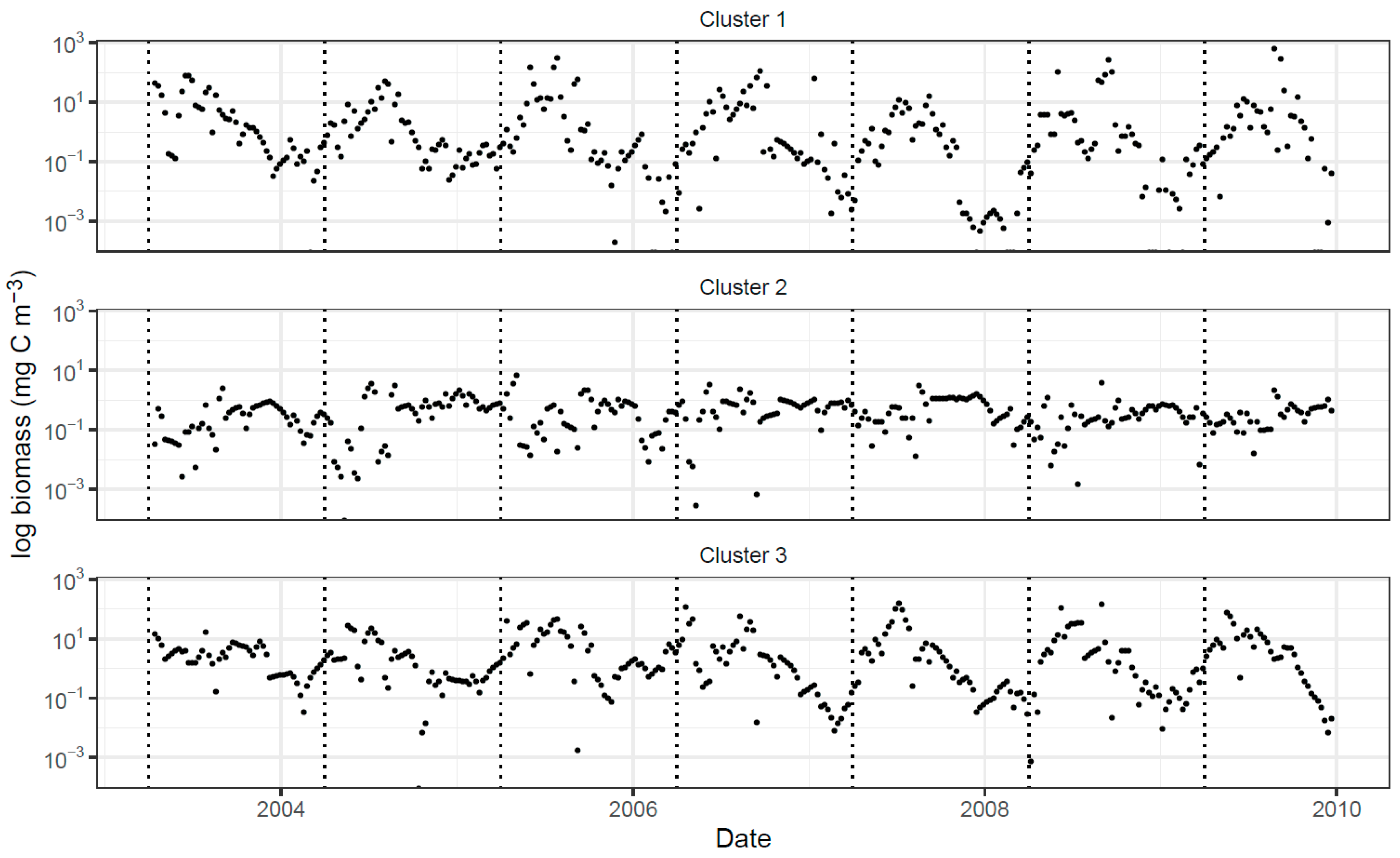
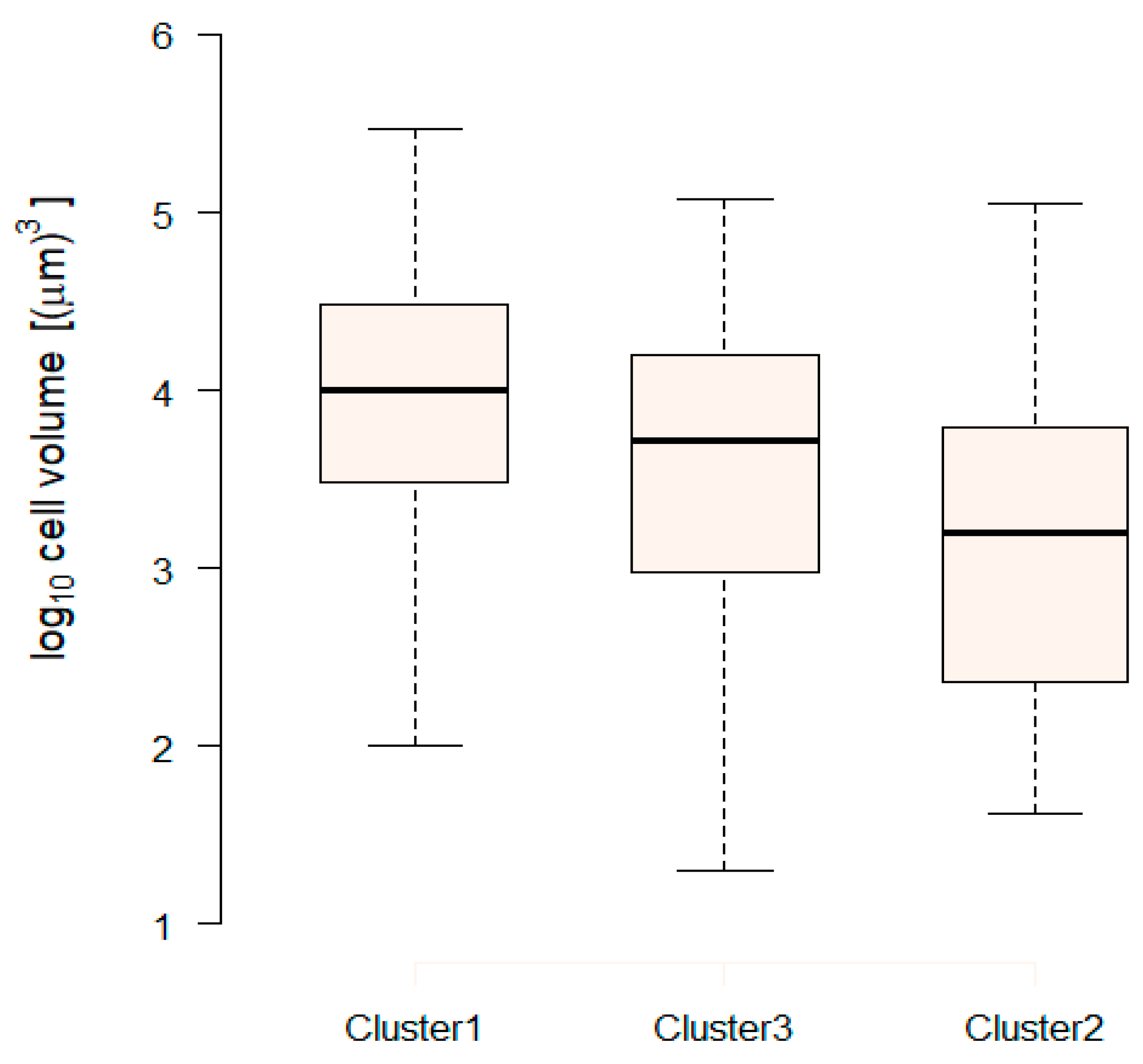
2.4.3. Extraction of Cluster-Specific Trait Values and Total Biomass Prediction

We used the Bayesian model of cluster-level biomass dynamics described by Equations (1)–(3) to extract cluster-specific trait values and predict the total biomass using three different sets of clusters. (1) The functional types represented in the data (diatom, dinoflagellate), (2) the three clusters generated by our method, and (3) the aggregate biomass of all species irrespective of functional type, herein referred to as total biomass. Drawing on our previous experience with the Station L4 data [8,9,24], we defined relatively informative priors for some of the model parameters. We assigned Gamma priors with shape parameter 6 and scale parameter 3 independently to cluster-specific intrinsic growth rates, r g , and carrying capacities, k g , and placed standard normal priors independently on the temperature effects, β g , 1 , and salinity effects, β g , 2 . We assigned positively truncated normal priors with mean zero and variance 0.01 and 1, on the nitrogen and silicate half-saturation constants, respectively. Estimation of the irradiance half-saturation constant from observation time series required well-constrained priors. We assigned to the irradiance half-saturation constants positively truncated normal priors centered at 15-mol m 2   d 1 . In order to assess the model sensitivity to prior inputs under the different clustering schemes, we considered a strong prior with prior variance 20, and a relatively less informative counterpart with prior variance 100, on the premise that the prior will be more influential under a clustering that conveys less information on the underlying factors and vice-versa.
We carried out the model fitting by MCMC simulation through OpenBUGS. We ran 10,000 iterations of three parallel Markov chains following a burn-in period of 6000 iterations and applied a thinning factor of 20 to the post burn-in samples. We assessed the convergence of the Markov chains informally through visual inspection of the trace plots and autocorrelation plots, and formally through the Gelman-Rubin statistic [30].
The posterior estimates of trait values differ widely between taxa under both the functional type typology and the trait-based grouping (Figure 4). Under the trait-based grouping, Cluster 1 dominated by diatoms has the highest intrinsic growth rate with a doubling time of 2 days, followed by Cluster 3 with a doubling time of 4 days. Cluster 3, which essentially combines biomass contributions from one third of the diatoms and all dinoflagellates except Prorocentrum balticum, stands out as the most responsive to changing environmental conditions with a positive response to increasing temperature and a negative response to increasing salinity (Figure 4b,c). Cluster 2, which mostly integrates biomass from a few diatoms and roughly half of the Prorocentrum balticum biomass (see assignment probabilities in Table A2, Appendix A) has the lowest intrinsic growth rate with a doubling time of 8 days, and exhibits the least sensitivity to environmental changes. This partly explains the weak seasonal cycles in the log-biomass of Cluster 2 as opposed to the other two clusters (Figure 3).
Under the functional type typology, the diatoms have, as a group, a slightly higher intrinsic growth rate than dinoflagellates with a mean doubling time of 2.5 days versus 3 days for dinoflagellates (Figure 4a). The temperature coefficient is negative and the salinity coefficient is roughly zero for diatoms (Figure 4b,c), implying that the optimal growth temperature at Station L4 for this group of diatoms is lower than the average temperature over the study period. The dinoflagellate biomass is highly sensitive to changing environmental conditions with positive response to increasing temperature and negative response to increasing salinity (Figure 4b,c), implying higher dinoflagellate biomass accumulation at higher temperatures and lower salinity than the average values over the study period, in line with findings from previous analyses of the Station L4 data [8].
Under the single cluster aggregation, the biomass dynamics model does not distinguish traits across species and models total diatom and dinoflagellate biomass, similar to many biogeochemical models that resolve only a single ‘large’ phytoplankton species. The intrinsic growth rate of the total biomass is intermediate between the growth rates of three clusters under the trait-based clustering and between those of the diatom and dinoflagellate biomass under the functional type grouping, with a doubling time slightly below 3 days (Figure 4a). The temperature and salinity coefficients are roughly null (Figure 4b,c).
The posterior distributions of half-saturation constants for resource acquisition (Figure 4) reveal tradeoffs across clusters of species (Figure 4d–f). Under the trait-based clustering, Cluster 2 has, on average, the highest irradiance half-saturation constant and the lowest silicate half-saturation constant. Cluster 3 has a very low nitrogen half-saturation constant and a relatively high silicate half-saturation constant. Cluster 1 has, on average, the highest nitrogen and silicate half saturation constants and the second largest half-saturation constant for irradiance. Under the functional type grouping, dinoflagellates have, on average, lower irradiance, nitrogen and silicate half-saturation constants than diatoms. Under the total biomass aggregation, the nitrogen half-saturation constant exhibits a large posterior uncertainty reflected in a wider credible interval (Figure 4e). The irradiance and silicate half-saturation constants echo those of diatoms under the functional type grouping (Figure 4d,f), which is not surprising since diatoms account for over 80% of the total biomass. The posterior distributions of trait values were under the trait-based clustering robust to the prior input, whereas under the functional type clustering, the posterior distribution of the irradiance half-saturation constant K E was unrealistically low (near zero) for dinoflagellates when assuming the relatively non-informative N + ( 15 ,   100 ) prior on K E (results not shown), where N + ( μ ,   σ 2 ) denotes the positively truncated Gaussioan with mean μ and variance σ 2 . We only report the results based on independent N + ( 15 ,   20 ) for the cluster-specific irradiance half-saturation constants under all clustering schemes.
We evaluated the performance of the Bayesian time series model for predicting the total biomass under our three clustering schemes through root mean squared prediction errors (RMSPEs). The posterior means (and standard deviations) of the RMSPEs obtained under the trait-based, functional-type, and total biomass clustering were 1.39 (0.12), 6.68 (1.24) and 1.37 (0.10), respectively. The RMSPEs under the trait-based and total biomass groupings were similar and roughly 5-fold lower than under the functional-type clustering.

3. Discussion

We developed a Bayesian model of phytoplankton biomass dynamics and analyzed a long-term series of weekly species-specific data collected at Station L4 in the Western English Channel, UK. In addition to the usual functional type categorization of phytoplankton species, we generated a trait-based clustering by building a three-component Gaussian mixture model using species scores on the leading principal components of occurrence traits as clustering features. Being soft in nature, the GMM clustering allows each species to belong to multiple clusters with different cluster assignment probabilities or cluster responsibilities summing to one. Our biomass predictions from the trait-based clustering were superior to the predictions from the functional-type clustering. Under relatively constrained priors, trait values for the three trait-based clusters showed variation similar to the results from the functional-type clustering, both of which were more informative than the trait values for aggregate biomass (Figure 4). This demonstrates the utility of subdividing total phytoplankton biomass into biologically meaningful clusters and underscores the need for exploring clustering schemes other than those determined strictly by taxonomic identity or biogeochemical role.
The maximum a posteriori clustering solution assigning each species to the cluster with the highest responsibility for the species’ feature vector partitioned the 74 species under consideration into three clusters with different characteristics. Cluster 1, the second largest cluster in terms of the number of species with twenty-six species, was comprised exclusively of diatoms. The largest cluster with thirty-five species, Cluster 3, combined all- dinoflagellates but Prorocentrum balticum and a third of the diatoms under consideration. Prorocentrum balticum, the only dinoflagellate excluded from Cluster 3, formed with twelve diatoms the smallest cluster, Cluster 2. The two large clusters (Cluster 1, 3) are clearly separated in the plane determined by the first two principal components PC1 and PC2 of occurrence traits. The species belonging to Cluster 2 fell in a narrow band between the two large clusters (Figure 2). The distribution of species in the trait-based clusters corroborates the documented diversity of diatoms [38] and the broadness of their ecological niche as a group. On the other hand, the restriction of all the dinoflagellates under consideration except Prorocentrum balticum to a single cluster suggests that their ecological niches overlap extensively. While balticum literally means, “pertaining to the Baltic sea”, Prorocentrum balticum is a cosmopolitan species found in cold temperate to tropical waters worldwide [39]. Adaptation to cold temperatures may partly explain its niche segregation from the bulk of dinoflagellates, as dinoflagellates generally thrive in warmer stratified and nutrient-poor waters.
We expect species of different clusters to differ in some other aspects. Looking at the cell volume of individual species, we discovered that species in the three clusters exhibit different cell volume distributions, with relatively larger cells in Cluster 1 followed by Cluster 3, and smaller cells in Cluster 2 (Figure 5). Size differences have far-reaching implications including differential grazing pressure: smaller species undergo a tighter grazing constantly keeping their biomass in check. This may partly explain the extended periods of near-constant log-biomass for Cluster 2, in contrast with the sustained seasonal cycles exhibited by the log-biomass of Cluster 1 and Cluster 3 (Figure 3).
The results of our trait-based clustering support the patterns of seasonal succession at Station L4. Cluster 1 species appearing in Table A1 are typical of the spring/autumn; Cluster 2 (Table A2) contains several species that are more typical of winter (e.g., Odontella mobiliensis and Pararlia sulcata) and early spring (Skeletonema costatum) when temperatures are low and turbulence is high. Cluster 3 species (listed in Table A3) such as smaller diatoms of the genus Rhizosolenia and Pseudo-Nitzschia, and the bulk of the dinoflagellates especially Karenia mikimotoi, generally reflect summer conditions when temperatures are warm [22].
We used the Bayesian model of biomass dynamics and the L4 data to examine, in connection with trait value characterization and biomass prediction, the tradeoffs encountered when aggregating biomass according to our trait-based clustering versus functional types and all species in a single cluster (total biomass). The model adequately estimated trait values under our trait-based clustering and proved robust to prior inputs. Under the functional type grouping however, the model required well-constrained priors, particularly on the irradiance half-saturation constant, to identify trait values. By consistently aggregating species with similar traits, our trait-based clustering provides a practical basis for exploring community-environment relationships. Within a functional type, species may have distinct and even conflicting environmental responses, as is the case for Prorocentrum balticum and the rest of dinoflagellates under study or for diatom species assigned to different clusters. Aggregating the biomass of species with conflicting trait will result in a weak community-environment relationships and inflated prediction errors, which explains the high model sensitivity to prior inputs and poor predictive performance of the Bayesian model of biomass dynamics under the functional type grouping.

4. Conclusions

Phytoplankton communities are extremely diverse and species-level abundance or biomass data are typically sparse, prompting the need to aggregate species into a few biologically meaningful groups when developing models to project biomass or characterize traits However, the choice of the applicable taxonomic resolution depends critically on the issue being addressed [40]. Phytoplankton functional types are valuable proxies for biogeochemical functions, but biomass prediction under the functional type clustering is prone to large prediction error since functional types combine species with very different or even contrasting traits. Our analysis of the L4 data demonstrates that grouping species by occurrence traits rather than the usual functional type labels can greatly enhance the characterization of traits used in biogeochemical models and improve the predictive accuracy of the biomass dynamics model. The trait-based clustering technique presented here applies to monitoring data from species-rich communities such as plankton assemblages for which data sparsity is ubiquitous. However, the idea is also applicable to observational time series with no missing data. For such data, the trait-based clustering can be generated by fitting the Bayesian model of biomass dynamics (Equations (1)–(4)) to species-level data and building a GMM with appropriate number of components on top of trait values characterizing species-environment relationships or their projections in a low dimensional space of leading principal components.
Projections of changes in phytoplankton communities and biogeochemical cycling typically rely on mechanistic models of phytoplankton productivity parameterized with traits [15]. As a result, trait-based approaches hold great promise for analyzing the biomass dynamics of species-rich communities and predicting the community response to environmental changes, which is highly valuable in the context of ongoing climate change.

Supplementary Materials

The following are available online at https://www.mdpi.com/1424-2818/12/8/295/s1, Figure S1: Log-likelihood of the EM model against the EM iteration number.

Author Contributions

Conceptualization, C.M.M. and A.J.I.; methodology, C.M.M. and A.J.I.; validation, Z.V.F., C.E.W. and A.J.W.; formal analysis, C.M.M.; writing—original draft preparation, C.M.M., A.J.I., Z.V.F. and C.E.W.; writing—review and editing, C.M.M., A.J.I., Z.V.F. and C.E.W.; supervision, A.J.I. and Z.V.F.; project administration, A.J.I.; funding acquisition, A.J.I. All authors have read and agreed to the published version of the manuscript.

Funding

This work was supported by the Simons Collaboration on Computational Biogeochemical Modeling of Marine Ecosystems/CBIOMES (Grant ID: 549935, AJI). C.E.W. was funded through the UK Natural Environment Research Council’s National Capability Long-term Single Centre Science Programme, “Climate Linked Atlantic Sector Science”, grant number NE/R015953/1, and is a contribution to Theme 1.3—Biological Dynamics.

Acknowledgments

Phytoplankton biomass and environmental data were provided by the Plymouth Marine Laboratory’s Western Channel Observatory www.westernchannelobservatory.org.uk, which was funded as part of the UK’s Natural Environmental Research Council’s National Capability.

Conflicts of Interest

The authors declare no conflict of interest.

Appendix A

As a soft or probabilistic clustering method, the GMM provides assignment probabilities of each species to every cluster. For visualization purposes, we considered the maximum a posteriori clustering solution assigning each species to the cluster with highest responsibility for its feature vector. More specifically, the maximum a posteriori solution assigns species s with feature vector x s to the cluster with highest responsibility for x s . Table A1, Table A2 and Table A3 show the species assigned to Cluster 1, Cluster 2 and Cluster 3 respectively, along with their functional types and assignment probabilities to all Clusters.
Table A1. List of species assigned to Cluster 1 by the maximum a posteriori clustering solution, their functional types, and their assignment probabilities to the three clusters. This cluster is the second largest in terms of the number of species with 26 species all of which are diatoms.
SpeciesFunctional TypeCluster Responsibilities
Cluster 1Cluster 2Cluster 3
Guinardia delicatuladiatom0.980.000.02
Meuniera membranaceadiatom1.000.000.00
Cerataulina pelagicadiatom1.000.000.00
Thalassiosira 10 µmdiatom0.700.180.12
Eucampia zodiacusdiatom1.000.000.00
Thalassionema nitzschioidesdiatom0.980.000.02
Guinardia striatadiatom0.500.450.05
Guinardia flaccidadiatom0.980.000.02
Dactyliosolen fragilimusdiatom0.960.000.04
Chaetoceros densusdiatom0.860.000.14
Corethron criophilumdiatom0.590.000.41
Ditylum brightweldiatom0.600.400.00
Rhizosolenia imbricata 5 µmdiatom0.970.000.03
Rizosolenia imbricata 15 µmdiatom0.680.000.32
Thalassiosira rotuladiatom0.990.000.01
Thalassiosira 20 µmdiatom0.760.000.24
Rhizoselenia styliformisdiatom0.880.000.12
Rhizosolenia setigera 25 µmdiatom0.770.230.00
Pseudo-nitzschia pungensdiatom0.990000.01
Chaetoceros socialisdiatom0.640.220.14
Thalassiosira punctigeradiatom1.000.000.00
Small pennatediatom0.870.110.02
Proboscia truncatadiatom0.990.010.00
Leptocylindrus mediterraneusdiatom1.000.000.00
Proboscia alatadiatom0.470.450.08
Detonula pumiladiatom1.000.000.00
Table A2. List of species assigned to Cluster 2 by the maximum a posteriori clustering solution, their functional types, and their assignment probabilities to the three clusters. This cluster is the smallest in terms of the number of species. It involves 12 diatoms and a single dinoflagellate namely Prorocentrum balticum.
SpeciesFunctional TypeCluster Responsibilities
Cluster 1Cluster 2Cluster 3
Paralia sulcatadiatom0.000.790.21
Diplomesis cabrodiatom0.000.780.22
Chaetoceros debilisdiatom0.200.540.26
Proboscia alata 5µmdiatom0.000.840.16
Chaetoceros danicusdiatom0.240.480.28
Nitzschia sigmoideadiatom0.200.640.17
Roperia tesselatadiatom0.040.790.17
Skeletonema costatumdiatom0.030.950.02
Chaetoceros affinisdiatom0.410.440.15
Odontella mobiliensisdiatom0.020.970.01
Pleurosigma planctonicumdiatom0.330.520.15
Chaetoceros simplexdiatom0.170.490.34
Prorocentrum balticumdinoflagellate0.340.480.18
Table A3. List of species assigned to Cluster 3 by the maximum a posteriori clustering solution, their functional types, and their assignment probabilities to the three clusters. This cluster is the largest in terms of the number of species with 35 species and involves all dinoflagellates except Prorocentrum balticum.
SpeciesFunctional TypeCluster Responsibilities
Cluster 1Cluster 2Cluster 3
Nitzschia closteriumdiatom0.000.001.00
Pseudo-nitzschia delicatissimadiatom0.040.040.96
Pleurosigmadiatom0.000.001.00
Pseudo-nitzchia seriatadiatom0.000.001.00
Lauderia annulatadiatom0.220.000.78
Navicula distansdiatom0.050.000.95
Leptocylindrus danicusdiatom0.030.000.97
Rhizosolenia setigera 5µmdiatom0.170.040.79
Navicula sp. diatom0.120.370.51
Leptocylindrus minimusdiatom0.010.010.98
Chaetoceros decipiensdiatom0.080.020.90
Pennate 50µmdiatom0.040.010.95
Rhizosolenia imbricata 10µmdiatom0.030.000.97
Podosira stelligeradiatom0.000.480.52
Thalassiosira 4µmdiatom0.000.001.00
Bacillaria paradoxadiatom0.250.230.52
Pennate 30µmdiatom0.000.001.00
Coscinodiscus radiatusdiatom0.250.050.70
Psammodictyon panduriformediatom0.000.001.00
Ceratium fususdinoflagellate0.010.000.99
Ceratium horridumdinoflagellate0.000.001.00
Ceratium lineatumdinoflagellate0.010.000.99
Ceratium triposdinoflagellate0.000.001.00
Dinophysis acuminatadinoflagellate0.000.001.00
Karenia mikimotoidinoflagellate0.000.001.00
Gonyaulax spiniferadinoflagellate0.000.001.00
Gymnodium sp.dinoflagellate0.020.000.98
Gymnodium cf. pygmaeumdinoflagellate0.000.001.00
Mesoporos perforatusdinoflagellate0.000.001.00
Micranthodinium sp.dinoflagellate0.000.001.00
Prorocentrum micansdinoflagellate0.000.001.00
Prorocentrum minimumdinoflagellate0.160.000.84
Prorocentrum triestinumdinoflagellate0.070.000.93
Scripsiella trochoideadinoflagellate0.000.001.00
Scripsiella sp. cystdinoflagellate0.080.000.92

References

  1. Sournia, A.; Chretiennot-Dinet, M.-J.; Ricard, M. Marine phytoplankton: How many species in the world ocean? J. Plankton Res. 1991, 13, 1093–1099. [Google Scholar] [CrossRef]
  2. Tuljapurkar, S.; Caswell, H. Structured Population Models in Marine, Terrestrial and Freshwater Systems; Chapman & Hall: New York, NY, USA, 1997. [Google Scholar]
  3. Falkowski, P.G.; Katz, M.E.; Knoll, A.H.; Quigg, A.; Raven, J.A.; Schofield, O.; Taylor, F.J.R. The evolution of modern eukaryotic phytoplankton. Science 2004, 305, 354–360. [Google Scholar] [CrossRef] [Green Version]
  4. Blaum, N.; Mosner, E.; Schwager, M.; Jeltsch, F. How functional is functional? Ecological groupings in terrestrial animal ecology: Towards an animal functional type approach. Biodivers. Conserv. 2011, 20, 2333–2345. [Google Scholar] [CrossRef]
  5. Yoshio, M.; Yasuhiro, Y.; Takafumi, H.; Hideyuki, N. Competition and community assemblage dynamics within a phytoplankton functional group: Simulation using an eddy-resolving model to disentangle deterministic and random effects. Ecol. Model. 2017, 343, 1–14. [Google Scholar]
  6. Le Quéré, C.; Harrison, S.P.; Prentice, I.C.; Buitenhuis, E.T.; Aumont, O.; Bopp, L.; Claustre, H.; Cunha, L.C.D.; Geider, R.; Giraud, X.; et al. Ecosystem dynamics based on phytoplankton functional types for global ocean bio-geochemistry models. Glob. Chang. Biol. 2005, 11, 2016–2040. [Google Scholar]
  7. Irwin, A.J.; Finkel, Z.V. Phytoplankton functional types: A functional trait perspective. In Microbial Ecology of the Ocean; Kirchman, D.M., Gasol, J.M., Eds.; Wiley: Hoboken, NJ, USA, 2016. [Google Scholar]
  8. Mutshinda, C.M.; Finkel, Z.V.; Widdicombe, C.E.; Irwin, A.J. Phytoplankton traits from long-term oceanographic time-series. Mar. Ecol. Prog. Ser. 2017, 576, 11–25. [Google Scholar] [CrossRef]
  9. Mutshinda, C.M.; Finkel, Z.V.; Widdicombe, C.E.; Irwin, A.J. Bayesian inference to partition determinants of community dynamics from observational time series. Community Ecol. 2019, 20, 238–251. [Google Scholar] [CrossRef]
  10. Nogueira, E.; Ibanez, F.; Figueiras, F.G. Effect of meteorological and hydrographic disturbances on the microplankton community structure in the Ría de Vigo (NW Spain). Mar. Ecol. Prog. Ser. 2000, 203, 23–45. [Google Scholar] [CrossRef]
  11. Bode, A.; Estevez, M.G.; Varela, M.; Vilar, J.A. Annual trend patterns of phytoplankton species abundance belie homogeneous taxonomical group responses to climate in the NE Atlantic upwelling. Mar. Environ. Res. 2015, 110, 81–91. [Google Scholar] [CrossRef]
  12. Mutshinda, C.M.; Finkel, Z.V.; Irwin, A.J. Which environmental factors control phytoplankton populations? A Bayesian variable selection approach. Ecol. Model. 2013, 269, 1–8. [Google Scholar] [CrossRef]
  13. Shimoda, Y.; Arhonditsis, G.B. Phytoplankton functional type modelling: Running before we can walk? A critical evaluation of the current state of knowledge. Ecol. Model. 2016, 320, 29–43. [Google Scholar] [CrossRef]
  14. McGill, B.; Enquist, B.; Weiher, E.; Westoby, M. Rebuilding community ecology from functional traits. Trends Ecol. Evol. 2006, 21, 178–185. [Google Scholar] [CrossRef]
  15. Litchman, E.; Klausmeier, C.A. Trait-based community ecology of phytoplankton. Ann. Rev. Ecol. Evol. Syst. 2008, 39, 615–639. [Google Scholar] [CrossRef] [Green Version]
  16. Pomati, F.; Nizzetto, L. Assessing triclosan-induced ecological and trans-generational effects in natural phytoplankton communities: A trait-based field method. Ecotoxicology 2013, 22, 779–794. [Google Scholar] [CrossRef] [PubMed] [Green Version]
  17. Krause, S.; Le Roux, X.; Niklaus, P.; Van Bodegom, P.M.; Lennon, J.T.; Bertilsson, S.; Grossart, H.-P.; Philippot, L.; Bodelier, P.L.E. Trait-based approaches for understanding microbial biodiversity and ecosystem functioning. Front. Microbiol. 2014, 5, 251. [Google Scholar] [PubMed]
  18. Kruk, C.; Devercelli, M.; Huszar, V.L.M.; Hernández, E.; Beamud, G.; Diaz, M. Classification of Reynolds phytoplankton functional groups using individual traits and machine learning techniques. Freshw. Biol. 2017, 62, 1681–1692. [Google Scholar] [CrossRef]
  19. Salguero-Gómez, R.; Violle, C.; Gimenez, O.; Childs, D. Delivering the promises of trait-based approaches to the needs of demographic approaches, and vice versa. Funct. Ecol. 2018, 32, 1424–1435. [Google Scholar] [CrossRef] [Green Version]
  20. Weithoff, G.; Beisner, B.E. Measures and Approaches in Trait-Based Phytoplankton Community Ecology—From Freshwater to Marine Ecosystems. Front. Mar. Sci. 2019, 6, 40. [Google Scholar] [CrossRef] [Green Version]
  21. Follows, M.J.; Dutkiewicz, S.; Grant, S.; Chisholm, S.W. Emergent Biogeography of Microbial Communities in a Model Ocean. Science 2007, 315, 1843–1846. [Google Scholar] [CrossRef] [Green Version]
  22. Widdicombe, C.; Eloire, D.; Harbour, D.; Harris, R.; Somerfield, P. Long-term phytoplankton community dynamics in the Western English Channel. J. Plankton Res. 2010, 32, 643–655. [Google Scholar] [CrossRef] [Green Version]
  23. Menden-Deuer, S.; Lessard, E.J. Carbon to volume relationships for dinoflagellates, diatoms, and other protest plankton. Limnol. Oceanogr. 2000, 45, 569–579. [Google Scholar] [CrossRef] [Green Version]
  24. Mutshinda, C.M.; Finkel, Z.V.; Widdicombe, C.E.; Irwin, A.J. Ecological equivalence of species within phytoplankton functional groups. Funct. Ecol. 2016, 30, 1714–1722. [Google Scholar] [CrossRef]
  25. Mutshinda, C.M.; O’Hara, R.B.; Woiwod, I.P. What drives community dynamics? Proc. R. Soc. Lond. B 2009, 276, 2923–2929. [Google Scholar] [CrossRef] [Green Version]
  26. Mutshinda, C.M.; O’Hara, R.B.; Woiwod, I.P. A multispecies perspective on ecological impacts of climatic forcing. J. Anim. Ecol. 2011, 80, 101–107. [Google Scholar] [CrossRef] [PubMed] [Green Version]
  27. Liebig, J. Organic Chemistry in Its Applications to Agriculture and Physiology; Taylor and Walton: London, UK, 1840. [Google Scholar]
  28. van der Ploeg, R.R.; Kirkham, M. On the origin of the theory of mineral nutrition of plants and the law of the minimum. Soil Sci. Soc. Am. J. 1999, 63, 1055–1062. [Google Scholar] [CrossRef] [Green Version]
  29. McCarthy, M. Bayesian Methods in Ecology; Cambridge University Press: New York, NY, USA, 2007. [Google Scholar]
  30. Gelman, A.; Carlin, J.B.; Stern, H.S.; Dunson, D.B.; Vehtari, A.; Rubin, D.B. Bayesian Data Analysis, 3rd ed.; Chapman & Hall: London, UK, 2013. [Google Scholar]
  31. Gilks, W.R.; Richardson, S.; Spiegelhalter, D.J. Markov Chain Monte Carlo in Practice; Chapman & Hall: London, UK, 1996. [Google Scholar]
  32. Thomas, A.; O’Hara, R.B.; Ligges, U.; Sturtz, S. Making BUGS open. R News 2006, 6, 12–17. [Google Scholar]
  33. Mutshinda, C.M. Markov chain Monte Carlo-based Bayesian analysis of binary response regression, with illustration in dose-response assessment. Mod. Appl. Sci. 2009, 3, 19–29. [Google Scholar] [CrossRef] [Green Version]
  34. Dempster, A.P.; Laird, N.M.; Rubin, D.B. Maximum likelihood from incomplete data via the EM algorithm. J. R. Stat. Soc. B 1977, 39, 1–38. [Google Scholar]
  35. Redner, R.A.; Walker, H.F. Mixture Densities, Maximum Likelihood and the EM Algorithm. SIAM Rev. 1984, 26, 195–239. [Google Scholar] [CrossRef]
  36. R Development Core Team. R: A Language and Environment for Statistical Computing; R Foundation for Statistical Computing: Vienna, Austria, 2019. [Google Scholar]
  37. Benaglia, T.; Chauveau, D.; Hunter, D.R.; Young, D. Mixtools: An R Package for Analyzing Finite Mixture Models. J. Stat. Softw. 2009, 32, 1–29. [Google Scholar] [CrossRef] [Green Version]
  38. Armbrust, E.V. The life of diatoms in the world’s oceans. Nature 2009, 459, 185–192. [Google Scholar] [CrossRef] [PubMed]
  39. Dodge, J.D. The Prorocentrales (Dinophyceae). II. Revision of the taxonomy within the genus Prorocentrum. Bot. J. Linn. Soc. 1975, 71, 103–125. [Google Scholar] [CrossRef]
  40. Bailey, R.C.; Norris, R.H.; Reynoldson, T.B. Taxonomic Resolution of Benthic Macroinvertebrate Communities in Bioassessments. J. N. Am. Benthol. Soc. 2001, 20, 280–286. [Google Scholar] [CrossRef]
Figure 1. Time plots of environmental variables at Station L4 between 14 April 2003 and 21 December 2009.
Diversity 12 00295 g001
Figure 2. Configuration of the 74 species in the plane defined by the first two principal components PC1 and PC2 of occurrence trait values. The shapes of plotting characters indicate the functional type of each species (filled circles for diatoms and filled triangles for dinoflagellates), while the colors indicate the cluster membership of each species with black, red and blue indicating Cluster 1, Cluster 2 and Cluster 3, respectively.
Diversity 12 00295 g002
Figure 3. Time plots of log-biomass for Cluster 1 (top), Cluster 2 (middle), and Cluster 3 (bottom) over the study period. Dashed vertical lines mark April 1 each year to highlight differences in seasonality between clusters 1 and 3.
Diversity 12 00295 g003
Figure 4. Estimated trait values for three different clustering schemes (total biomass, top; functional type clustering, middle; trait-based clustering, bottom) showing: (a) intrinsic growth rates; (b) temperature effect on growth rate; (c) salinity effect on the growth rate; (d) irradiance half-saturation constant; (e) nitrogen half-saturation constant; and (f) silicate half-saturation constant for each cluster of species. Error-bars (posterior mean ± 1 SD) represent 68% credible intervals around the posterior means (filled circles). These results are based on independent N + ( 15 ,   20 ) priors on cluster-specific irradiance half-saturation constants under our three clustering schemes.
Diversity 12 00295 g004
Figure 5. Box and whisker diagrams of log cell volume distributions in the three trait-based clusters based on the maximum a posteriori clustering solution. Each box plot shows the median (thick line), the interquartile range (box) and the full range of the distribution from 1.5 interquartile range below the first quartile to 1.5 interquartile range beyond the third quartile (whiskers). Clusters are arranged in order of decreasing medians.
Diversity 12 00295 g005
Table 1. Loadings of the environmental variables on the three leading principal components accounting for 76% of variation in presence-absence trait values across species. Bold numbers highlight the variables that dominate each principal component.
Variable PC1PC2PC3
Irradiance (PAR)0.66−0.190.53
Temperature0.67−0.06−0.25
Salinity0.020.140.14
Nitrogen0.230.94−0.07
Silicate0.11−0.19−0.02
Phosphate0.20−0.16−0.79

