Article

Freshwater Mussel Bed Habitat in an Alluvial Sand-Bed-Material-Dominated Large River: A Core Flow Sediment Refugium?

1
Department of Biological Sciences, Arkansas State University, P.O. Box 599, State University, Jonesboro, AR 72467, USA
2
Biology Department, Clarkson University, CU Box 5805, 8 Clarkson Ave, Potsdam, NY 13699, USA
3
The Nature Conservancy, New Paltz, New York, NY 12561, USA
*
Author to whom correspondence should be addressed.
Diversity 2020, 12(5), 174; https://doi.org/10.3390/d12050174
Submission received: 4 March 2020 / Revised: 30 March 2020 / Accepted: 23 April 2020 / Published: 28 April 2020

Abstract

:
Habitat degradation, organismal needs, and other effects influencing freshwater mussel declines have been subject to intense focus by conservationists for the last thirty plus years. While researchers have studied the physical habitat requirements and needs of mussels in small- to medium-sized rivers with variable levels of success, less research has been conducted on mussel habitat in larger non-wadeable rivers, especially at the reach scale, where core flow environmental conditions provide and maintain habitat for freshwater mussels. We designed a quasi-experimental observational field study to examine seven hydrologic energy and material variables laterally and longitudinally at Current and Extirpated mussel bed habitat reaches in lower White River, Arkansas, a large non-wadeable, sand-bed-material-dominated river. As expected, lateral and longitudinal hydrologic variable differences were identified within a reach. Mean velocity, bed velocity, the Froude number, and stream power were all significantly lower at Current mussel bed habitat stations within a sampling reach. Energy regime differences in shear stress and, marginally, stream power were higher at Extirpated mussel bed habitat reaches. Several factors emerged as important to mussel habitat in the White River. First, bed velocity warrants further exploration in terms of both flow strength and flow direction. Second, bedload appears to be the primary contributor to mussel habitat but requires additional exploration within the context of core and secondary flow pathway interactions. The combined empirical evidence from our study supports the flow refugium concept identified for mussel habitats in smaller systems but expands the concept to large non-wadeable streams and includes reach-scale refuge from sediment transport conditions.

1. Introduction

Habitat provides the template in which evolution forges characteristic life-history strategies across evolutionary spatiotemporal scales [1] and acts to filter out unsuccessful strategies, thereby controlling community composition [2,3]. Stream habitats are recognized as being organized hierarchically at spatiotemporal scales ranging from larger to smaller stream systems that successively encompass spatially smaller and temporally shorter segment systems, reach systems, pool/riffle systems, and microhabitat systems [4]. Each lower-level system and community is influenced by larger scales operating at higher geological spatiotemporal scales [4,5].
Understanding habitat degradation, organismal habitat needs, and other effects influencing freshwater mussel declines has been the focus of North American conservation organizations for the last thirty plus years [6,7]. How mussels, as individuals and as assemblages, interact with highly variable physical habitat requirements continues to be difficult to synthesize and remains a significant void of understanding [7]. Researchers have increased our knowledge base and addressed habitat conditions and degradation by investigating physical habitat requirements of mussels for small- and medium-sized streams and impounded areas of large (i.e., non-wadeable) streams with variable levels of success [8,9,10,11,12,13,14,15,16,17,18,19,20,21,22,23,24,25,26,27,28]. Fewer studies have investigated large-stream habitats [29,30,31,32,33,34,35]. In large alluvial streams in Arkansas, mussel beds (i.e., discrete, definable physical area inhabited by high densities of mussels, usually consisting of more than one species) can be found just downstream of run reach-scale habitats in the deeper lateral scour pool habitat continuing through the approach of glide habitat into riffle habitat (Figure 1) [36].
Within a larger non-wadeable river channel, there are multiple forces interacting with each other to produce a variety of hydrological flow conditions which can change with discharge levels [37,38]. These interactions, known as the core flow concept, create vortices causing water to flow in a variety of directions. The primary flow, herein referred to as the core, shifts position within the channel as stage and discharge fluctuate and, generally, is associated with the highest velocities in the downstream direction. Due to boundary layer interactions, among others, secondary flow pathways develop which, within a river bend, push surface water to the outside bank and water found near the substrate is pulled toward the inside bank (i.e., point bar). This effectively forms a spiral flow condition around the core and produces an area of down-welling near the outside bank (Figure 2). Meanwhile, a second cell of reverse flow develops along the outside bank; however, this condition is only present with smooth vertical banks and is not present with terraced banks [37,38]. The intensity of the secondary flow pattern is most prominent at moderate velocities with reduced effects during periods of low and high flow. These conditions also appear to influence the distribution of shear stress along the outside wall of the bend. During low and high flow discharge, shear stress is typically characterized as uniform due to increasing Reynold’s number (ratio of inertial forces to viscous forces) but becomes distorted during moderate flows. Drawing a link between hydraulic forces and river bed materials with resulting habitat features and biotic presence or absence is an area of promising exploration [39].
The White River of Missouri and Arkansas is species rich, with as many as 61 mussel species, and many were commercially important historically [40,41,42]. Imperiled species of the White River include the Federally protected Pink Mucket (Lampsilis abrupta), Scaleshell (Leptodea leptodon), Fat Pocketbook (Potamilus capax), and Rabbitsfoot (Theliderma cylindrica) [40,43]. In the mid-1990s, 110 historically harvested (i.e., based on commercial shell-taker interviews) mussel bed locations in the downstream portion of the White River from river kilometer (rkm) 0 to 418 were identified through commercial shell-taker interviews [44,45]. These beds were examined using qualitative scuba diving methods for each 110 bed reconnaissance and stratified random sampling of delineated beds via excavation of 1 m2 quadrats [44,45]. Of the 110 historically harvested beds, 51 extant beds were documented with 17 classified as major beds (mean mussel density > 10 m2, bed area > 500 m2) and 34 classified as minor beds (mean density > 10 mussels/m2, area < 500 m2); in either case, these beds were considered to consist of viable species-rich and demographically variable mussel assemblages [44,45]. Extant beds most often occurred in reach-scale habitats at the upstream limit of an outside bend extending downstream until active erosion was evident on the vertical banks. Extant beds were associated with the thalweg and firm stable gravel/sand or clay substrates. Meanwhile, 40 of the 59 remaining historically significant bed locations exhibited low densities (1–5 mussels/m2), and 19 beds appeared to have been extirpated (i.e., very few to no mussels observed). Three distinct regions were identified in the lower White River based on mussel bed species composition and habitat condition [44]. The Upper Region ranged from rkm 315 to 418 and possessed relatively stable bank and substrate conditions. The Middle Region from rkm 161 to 351 had relatively unstable bank and substrate conditions. The Lower Region, rkm 0–161, extended from the confluence with the Mississippi River upstream and had more stable banks and substrates. The Middle Region seemed the most at risk due to observed losses of commercial mussel beds, while the Lower Region appeared somewhat resistant to changes experienced within this system over the last century and still exhibits excellent examples of large river mussel fauna [40,44,46].
The objective of this study was to obtain quantitative reach-scale habitat (e.g., riffle, run, pool) information relating to hydrologic energy and bed material variables (i.e., channel slope, discharge, velocity, the Froude number, shear stress, stream power, and bedload) across seasons, regions, habitats, lateral position, and Current and Extirpated mussel beds in the large non-wadeable alluvial sand bed material-dominated lower White River, Arkansas. We anticipated differences in hydrologic variables between seasons, regions, Current and Extirpated beds, and within a reach. We expected these differences to be influenced primarily by local channel morphology characteristics such as sediment type, channel slope, and discharge and to result in a core flow refuge where mussel beds are likely to persist. Through this analysis, we also expected Current mussel bed locations to be characterized by areas of reduced near-bed velocities and to find areas categorized as Extirpated beds to be characterized by higher velocities and greater sediment transport conditions.

2. Materials and Methods
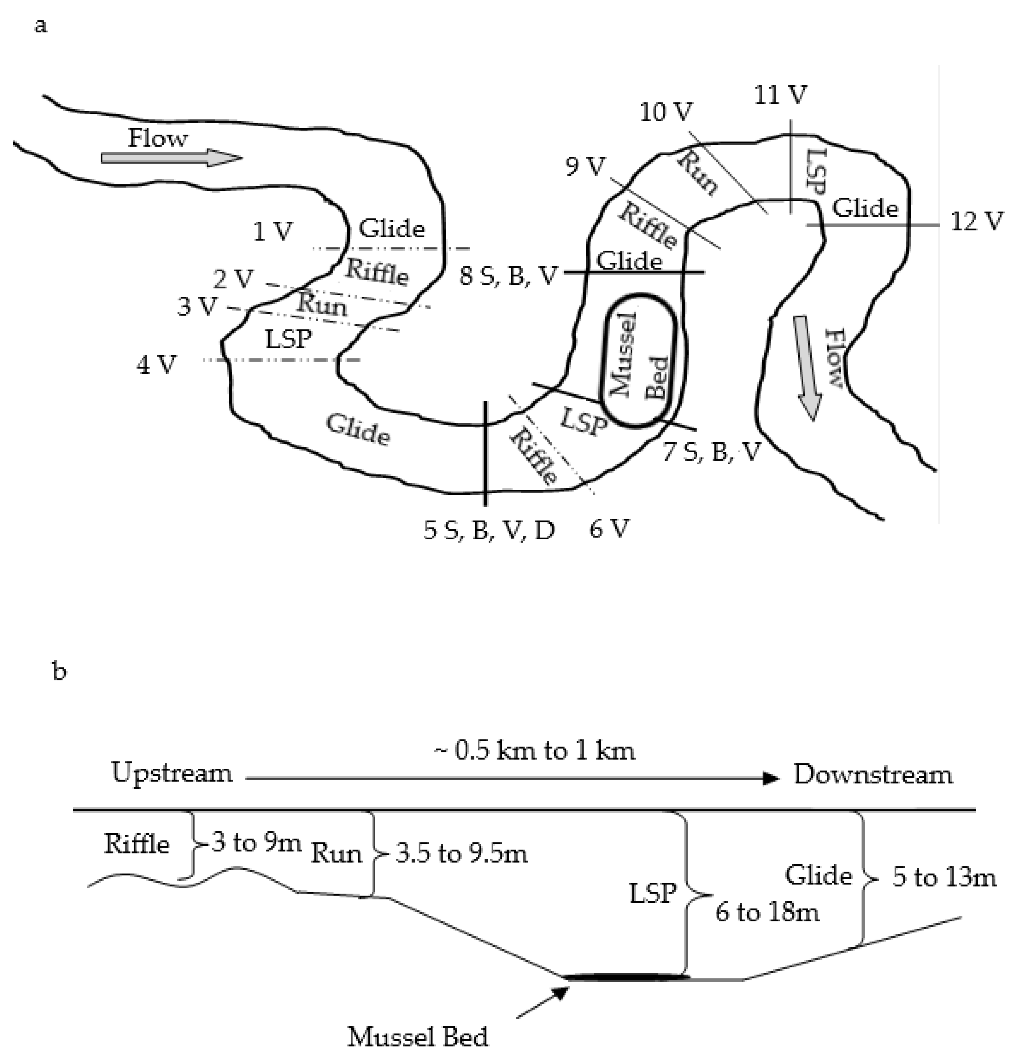
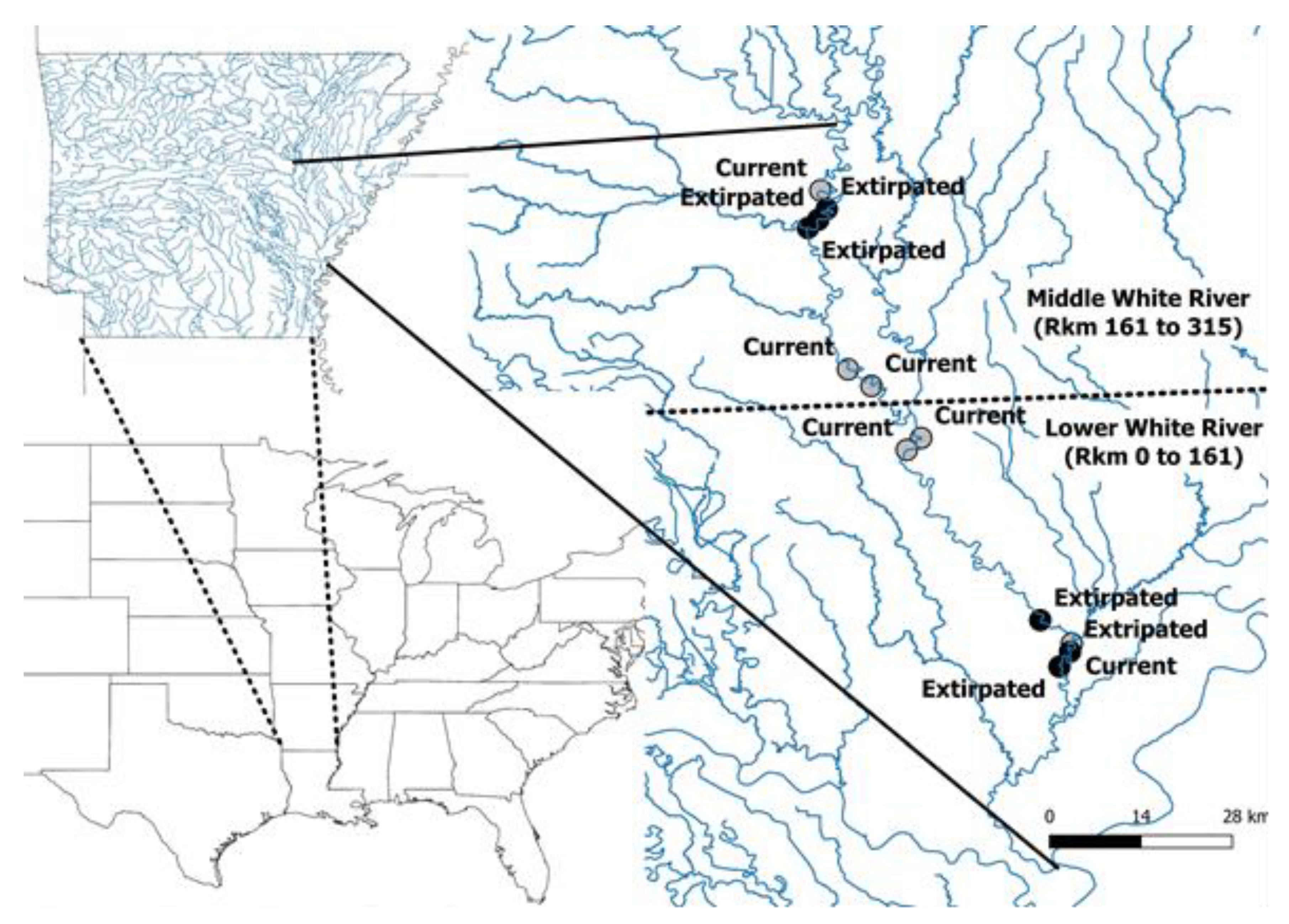
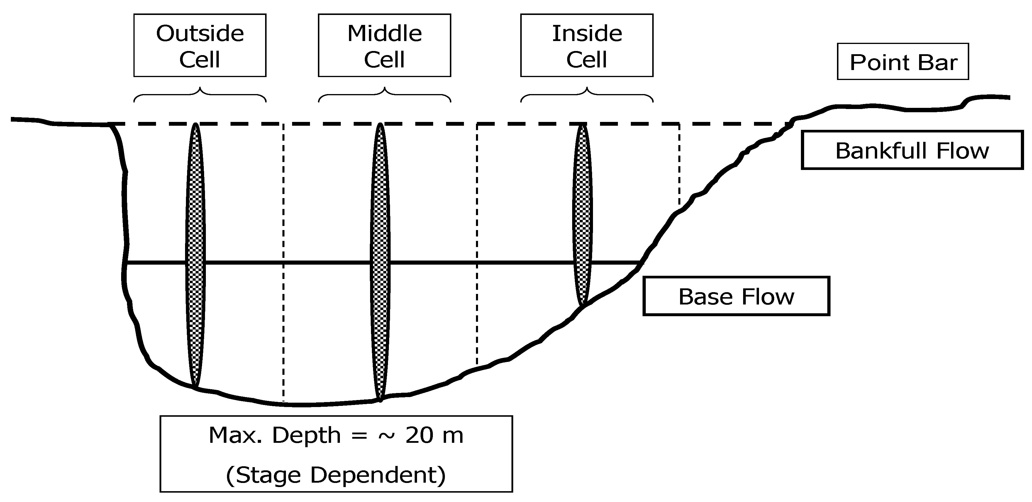
2.1. Study Area

The White River originates on the northern slope of the Boston Mountains (Ouachita-Ozark Interior Highlands geologic province) in northwestern Arkansas, is approximately 1210 km in length and has a drainage area of 72,500 km2 [47]. In the watershed, mean basin elevation is 656 feet, mean annual precipitation is 47.8 inches, and land uses derived from National Land Cover Database (NLCD) 2011 classes indicate very little developed land in the water shed (developed land 6.5%; mean impervious area 0.7%) [47]. In the Boston Mountains, the White River flows northeasterly into south-central Missouri, traversing the Springfield and Salem plateaus, and then takes a southeastward route back into Arkansas, where it exits the Ozark Plateaus flowing the last 420 rkm through the Mississippi Alluvial Plain. Physical and chemical characteristics of the river are influenced by a series of large, hypolimnetic release dams in upstream portions, a variety of land uses, and channel maintenance activities in the Lower Region [48]. The most downstream large hypolimnetic mainstem dam (Bull Shoals Lake, Arkansas) is in the Ozark Plateaus, the most downstream low head run-of-the-river dam (Batesville, Arkansas) is at ~rkm 420, and the most downstream hypolimnetic release dam on a tributary (Little Red River and Greers Ferry Lake, Arkansas) is at ~rkm 177.

2.2. Study Reach Identification

For this study, 12 river reaches were selected haphazardly, based on accessibility and safety considerations, from the Middle (n = 6) and Lower (n = 6) Regions based on the 110 mussel beds previously examined [44] (Figure 3). The Upper Region was eliminated due to low mussel densities (i.e., <10 individuals/m2) and logistical constraints (e.g., lack of boat launches and long boat trips). For each region, three Current high-density mussel beds (>10 individuals/m2 in areas >500 m2) and three Extirpated mussel beds [44] were selected with emphasis on balancing spatial distribution and considering sampling logistics (e.g., river access and boat travel). The 12 study reaches selected were qualitatively surveyed in 2004 via SCUBA to verify mussel densities and conditions remained similar to those documented; no quantitative data was recorded in 2004 [44].
Each study reach was delineated by referencing the most recent digital ortho-photographs, known GPS coordinates, and/or field truthing. Within each study reach, three transects (Figure 3) were established haphazardly (using professional judgement of habitat profile for placement) based on functional habitat type (i.e., riffle, run, lateral scour pool) [36,49]. Habitat classification was based on streambed characteristics identified by traversing the river both laterally and longitudinally, while noting depth patterns with a boat mounted Eagle CUDA™ 168 depth-finder. GPS coordinates were obtained using a Trimble GPS unit and recorded (Decimal degrees, NAD 83) for each habitat transect on either the right or left bank [upstream facing downstream (descending) perspective]. Global Positioning System coordinates were downloaded and processed through ArcMap 8.3 (ESRI, Redlands, California, CA, USA) allowing the production of individual site maps with transect coordinates.

2.3. Sampling

Sampling stations across each transect were determined by dividing the wetted channel width into thirds to establish equidistant cells—hereafter, described as Inside (I), Middle (M), and Outside (O) (Figure 4). During high flow, channel width was used instead of wetted width due to complications of accessing and determining wetted width in areas of extensive flooding. Where banks were not visible, vegetation located on the top of bank was referenced and the bank edge determined via depth finder. Sampling occurred at the center of each of the three cell stations for each transect. Due to the challenge of returning to the precise sample location each time, cells were defined during each sampling event at each transect.
In order to capture a wide range of hydraulic conditions, field sampling occurred over three flow types, a Spring moderate flow (mid-June to mid-July 2004), an Autumn low flow (September 2004), and a Winter high flow (mid-December 2004 to early January 2005). Information collected included discharge (Q), velocity profile (VP), and bedload (B). Due to the number of stations sampled per reach (three stations each at three habitat transects; n = 9), time associated with travel, and water depth during moderate and high flow sampling efforts, typically only one reach was completed per day.

2.3.1. Channel Slope

Channel slope was determined using change in elevation across the reach length and dividing it by reach length [50]. We obtained this data from manual calculations using corresponding U.S. Geological Survey 7.5-min topographical maps.

2.3.2. Discharge

Discharge was calculated only at the riffle transect immediately upstream of the defined mussel bed area. Riffles were chosen because channel geometry tended to be more uniform than either the lateral scour pool (LSP) or glide, allowing for more accurate results. Velocity readings were taken and recorded at 0.8, 0.6, and 0.2 d, where d equals depth, and 1.0 d represents the stream bottom. Discharge was calculated using the velocity-area method, Q = VA, where Q is discharge (m3/s), V is the profile mean velocity (m/s), and A is the cross-sectional area of the wetted channel (m2). Mean V was determined using:
Vmean = 0.25(v0.2 + v0.8 + 2v0.6)
as described by Gordon et al. [50]. Discharge was referenced with the nearest United States Army Corps of Engineers stream gauging station [51]. Discharge frequencies, also known as return intervals, were determined using the stream analysis software RIVERMorph® (RiverMorph 2004; RIVERMorph LLC, Louisville, Kentucky) and downloaded data from the USGS stage recorders closest to the study reach.

2.3.3. Velocity

Velocity measurements were taken using a Marsh-McBirney Flow-MateTM at 1.0 m increments from the channel bottom to the water surface and recorded. Mean velocity was determined from the resulting profile information, and bed velocity was calculated as 0.70V, where V is the mean velocity of the profile [50]. However, it should be noted that bed velocity is based on a conversion from mean velocity, is autocorrelated with mean velocity, and should mimic mean velocity values and patterns.

2.3.4. The Froude Number

The Froude number, the ratio of inertial forces to gravitational forces, reflects general flow characteristics at a given cross-section and was calculated by the following:
Fr = V/√gD
where V is the mean velocity in units m·s−1, g is the gravity induced acceleration (9.8 m/s2), and D represents mean water depth in m [50]. Using a critical velocity for V could produce one of three possible flow conditions: Fr < 1 indicates flow with little ability to rearrange bedforms; Fr = 1 indicates critical flow, the point at which bedform rearrangement begins; Fr > 1 indicates a high capacity to rearrange channel bedform.

2.3.5. Shear Stress

Shear stress, the measure of force acting horizontally on a particle, was determined using the slope of vertical velocity log profile [50,52]. Shear stress was determined by:
To = p (V*)2
where To is shear stress (N/m2), p is the density of water and V* is the shear velocity. Shear velocity was determined by:
V* = b/5.75
where b is the slope of logarithmic velocity profile and 5.75 is a constant [50].

2.3.6. Stream Power

Stream power, the ability of a particular flow to do work (i.e., rearrange bedforms or transport sediment), was used to examine the erosive attributes of the channel at multiple stage or discharge levels [50]. For this project, stream power per unit of stream bed area (watts/m2), wa, was calculated as:
wa = To V
where To is shear stress, and V is the mean velocity.

2.3.7. Bedload

Bedload was collected using a BL-84 Helley-Smith sampler, a 29.5 kg (65 lb) sampler with an expansion ratio of 1.44, and a #3-mesh collection bag with 250-micron openings. Due to equipment loss, high flow samples from 4 sites were collected with a similar unit; however, the replacement had an expansion ratio of 3.22 and a #1 mesh bag with 250-micron openings; the difference in the devices was not expected to affect our results. Bedload samples were frozen until size fraction analysis was conducted.
Prior to size fraction analysis, bedload samples were thawed, transferred to a 20.32 cm pan, labeled with sample location and date information, and placed in a drying oven for 24 h at 60 °C. Size fraction analysis was accomplished using the 2.0 mm (#10), 0.85 mm (#20), 0.425 mm (#40), 0.25 mm (#60), 0.15 mm (#100), and 0.075 mm (#200) sieves and collection pan [53].
Bedload transport rates were calculated for each cell using the formula
Qbli = Mi/Wt
where Qbli is bedload discharge (g/m·s), M is the mass of the sample (g), W is the width of the nozzle opening in mm, i refers to the ith measurement point (Inside, Middle, Outside), and t refers to the measurement time interval [50]. Qbli is multiplied by the width of the cell sampled, and the cells are then summed across the transect
Qbl = WI(QBI) + WM(QBM) + WO(QBO)
where W is the cell width and I, M, and O represent lateral position along the transect.
Additional system components including total suspended sediment (TSS) concentration and loading, as well as channel planimetric form, were examined in this study. However, the results either failed to provide additional insight to the questions being addressed or mimicked the findings of other variables [54].

2.4. Statistical Analysis

Physical habitat conditions were compared both temporally and spatially. Variables were analyzed by multivariate ANOVA using JMP-In (V.4, SAS Institute, Cary, NC, USA). The factors for this analysis included season (Spring (moderate flow), Autumn (low flow), Winter (high flow)), segment (Middle and Lower), mussel bed type (Current and Extirpated), habitat (riffle, LSP, glide), and lateral position (I, M, and O) with all interactions examined. All results were analyzed and reported using an a priori alpha = 0.10 significance level (due to low sample size) and were sequentially Bonferroni corrected to adjust for performing a number of test with multiple comparisons [55]. Pair-wise comparisons were analyzed using the Tukey–Kramer honest significant difference (HSD) test, with a pair-wise error rate of 0.05. Pooled means for all habitat values by treatment are provided in Table A1, Table A2, Table A3, Table A4, Table A5, Table A6 and Table A7.

3. Results

3.1. Channel Slope

Channel slopes ranged from 0.000043 to 0.000063 m/m, with the lowest channel slopes occurring near Clarendon, AR, WR 096 and WR 094, and the highest slopes occurring at five other stations (Table 1), but they were not significantly different from each other (Two-way ANOVA: F3,11 = 0.76, p = 0.54). Slope throughout the entire Middle Region increased with downstream distance, but there was a decrease in slope at the upstream limit of the Lower Region.

3.2. Discharge

Overall, discharge (Q) showed statistically significant (Two-way ANOVA: F5,35 = 81.06, p < 0.0001) increase with downstream distance (Table 2) with significant interaction effects. For season, Autumn discharge sampling conditions were representative of baseflow conditions and ranged from 206.78 to 487.43 m3·s−1, Spring conditions were below bankfull and intermediate, ranging from 459.70 to 686.61 m3·s−1, and Winter conditions were representative of high flow, ranging from 732.90 to 1339.48 m3·s−1. All season effect combinations were significantly different with Winter greater than Spring which was greater than Autumn (Table 3). Season × region showed multiple significant interactions that were largely influenced by the seasonal effect (Table 3). Winter flow conditions had a return interval (i.e., likelihood of return to the same level) of 1 year.

3.3. Mean Velocity

Mean cell velocities over all reaches and seasons ranged from −0.06 to 1.41 m·s−1, with a mean velocity of 0.76 m·s−1 (Table 4), and were significantly different (Five-way ANOVA: F41, 337 = 11.52, p < 0.0001), with significant effects for all factors except bed type (Table 3 and Table 4). For Season, Autumn velocities were lowest, Spring velocities were intermediate, and Winter velocities were highest (Table 4), and all seasonal pair-wise comparisons were significantly different (Table 3). For Habitat, mean velocity at LSP was significantly less than mean velocity for Riffle; no other habitat effect differences were indicated. For lateral position, Middle mean velocity was significantly greater than both Inside and Outside (Table 4). One station, WR 147 Glide/Outside, was not sampled during Winter due to unsafe field conditions and was excluded from all velocity-based calculations. Effects between the Middle and Lower Regions were characterized by the Lower Region having a significantly greater mean velocity than the Middle Region (Table 3 and Table 4).

3.4. Bed Velocity

Mean bed velocity estimates ranged from −0.04 to 0.99 m·s−1 over all events and reaches and were significantly different (Five-way ANOVA: F41,322 = 11.16, p < 0.0001; Table 5) with significant effects for all factors except bed type (Table 3). Winter yielded significantly greater mean estimates than either Spring or Autumn (Table 4); Spring and Autumn were not statistically different (Table 3; Table 4). Mean bed velocities in LSP transects were significantly less than Riffle transects with no other differences occurring. Lateral position analysis of mean bed velocity indicated that the Middle cell was significantly greater than the Inner and Outer cells (Table 4). Lower Region mean bed velocity was significantly greater than Middle Region mean bed velocity. Differences in habitat × lateral position interactions were apparent with LSP/Outside bed velocity significantly less than all other cells except Glide/Inside and Riffle/Outside—between which there was no difference (Table 3; Figure 5).

3.5. Froude

Mean cell Froude numbers ranged from −0.01 to 0.26 across all reaches and sampling events and were significantly different (Five-way ANOVA: F32,322 = 7.64, p < 0.0001; Table 5), with the factors lateral position, season, and segment, and the interactions habitat × lateral position, habitat × season, and season × segment significantly different (Table 3 and Table 4). Autumn mean Froude numbers were significantly greater than both Spring and Winter. Outside Froude numbers were significantly lower than Inside or Middle; there was no difference between the Inside and Middle Froude numbers. For regions, Lower Froude numbers were significantly greater than Middle Froude numbers (Table 4).

3.6. Shear Stress

Shear stress estimates ranged from 0.00 to 224.29 N/m2 across all reaches and seasons and were significantly different (Five-way ANOVA: F 24,323 = 3.15, p < 0.0001; Table 5), with significant factors of season and bed type (Table 2 and Table 3). Lateral position × season was the only significant interaction (Table 3). Season analysis showed Autumn with significantly higher sheer stress than both Winter and Spring, with no difference between Winter and Spring. Bed type analysis showed shear stress significantly lower at Current beds by approximately 33%.

3.7. Stream Power

Stream power per unit width estimates ranged from 0.00 to 96.94 W/m across all reaches and were significantly different from each other (Five-way ANOVA: F32,322 = 2.85, p < 0.0001; Table 5). Significant differences were observed in the factors season and bed type, with multiple interactions identified (Table 2 and Table 3). Autumn stream power was significantly greater than either Spring or Winter. Bed type analysis indicated significantly greater mean stream power values at Extirpated beds than Current beds (Table 4).

3.8. Bedload Discharge

Mean Qbl ranged from 0.0 to 5502.0 g·s−1 across 12 reaches (Five-way ANOVA: F12,323 = 12.09, p < 0.0001; Table 5). Significantly different effects of season, habitat, and lateral position, and the interaction of habitat × lateral position were observed (Table 2 and Table 3). Season analysis revealed Winter samples were significantly higher than both Autumn and Spring samples, with Spring and Autumn not significantly different from each other (Table 4). Habitat effect analysis indicated that the mean Glide Qbl was significantly less than both LSP and Riffles, while LSP and Riffles were not significantly different from each other. All lateral positions were significantly different from each other, with Inside mean Qbl the greatest, Middle intermediate, and Outside lowest (Table 4; Figure 6).

3.9. Bedload Mean Particle Size

Bedload mean particle size ranged from 0.00 to 1.26 mm, with a mean of 0.40 mm (±0.22 mm SD), across all reaches, and there were no significant differences (Five-way ANOVA: F99, 323 = 1.04, p = 0.41; Table 3 and Table 5). Spring samples had the highest mean particle size, and both Autumn and Winter sample means were essentially the same (Table 4).

4. Discussion

This quasi-experimental (i.e., observational) field study examined the relationship between hydrological conditions at spatial (lateral and longitudinal locations) and temporal (seasonal) scales in river reaches that currently provide suitable habitat for high-density commercially harvestable mussel beds and reaches that formerly hosted commercially harvestable mussel beds. At a broad scale, we identified differences in seasons, segments, between reaches, and within reaches across three sampling events. The results indicated that the space used by mussels in this large, non-wadeable, sand-bed-material-dominated river represents areas of both flow and sediment refuge similar to the concepts suggested for wadeable streams [19]. For example, reaches harboring Current mussel beds were characterized by lower mean shear stress and mean stream power values. Further, within a reach, the mussel bed area (LSP/Outside) exhibited much lower velocity and sediment transport rates. However, due to the nature of our study (i.e., quasi-experimental and low sample size), we were unable to determine thresholds explaining the distributional pattern of Current versus Extirpated mussel beds. In fact, conditions at the beds during the study period may have not have any relation with past environmental conditions when the mussel beds became extirpated. In the following, we contextualize our findings for each hydraulic variable independently and integrate them into “the core flow model” [37,38]. Finally, we hypothesize how the conceptual model may affect the distribution of mussel beds in large rivers.

4.1. Channel Slope

Local slopes likely play a marginal role in habitat formation and maintenance but warrant more detailed exploration relating to freshwater mussel habitat [8]. The slope values determined for this project showed the typical decrease with downstream distance per the river continuum concept (RCC) [56]. Differences in slope, though not statistically significant, were identified within the study area and provide insight to the general characteristics of the study reaches. The unexpected change in slope at the upstream extent of the Lower Region is interesting, as there are exceptionally high-density mussel beds in the area [44]. An unusually wide channel was present upstream of WR 96, a possible association with a reduced slope. Though the larger reach-scale (~5 km) analysis of slope in this study revealed useful information, a local-scale (<0.5 km) analysis, such as LSP entrance and exit slopes, may be more appropriate for providing data significant to mussel bed distribution.

4.2. Discharge

Overall, discharge measurements were as expected both temporally (seasonal differences) and spatially (increasing downstream). Discharge variability in the lower White River during this study was influenced by four factors: (i) over bankfull volume conditions in the Lower Region; (ii) water levels falling when Lower Region reaches were sampled; (iii) variability in storms, dam release and other factors; (iv) effect of Mississippi River stage on White River backwater. The return interval of approximately 1 year identified for the Winter event was similar to other systems in the ecoregion [57] and discharge generally showed the predictable increase with downstream distance [58]. Flow return intervals indicate how frequently the high flow conditions might be experienced and provide a level of confidence that a flow anomaly was not captured during this study. A 1-year return interval indicates that biota, specifically mussels, are exposed to the reported conditions on a relatively regular (annual) basis and must be able to endure these conditions in order to maintain position in the substrate.

4.3. Velocity

Mean velocity values generally increase with downstream distance in our study area; however, this is somewhat unexpected as volume is increasing, but slope is similar to or decreasing, at least in the upstream portion of the Lower Region. This is likely attributable to localized facet slopes and/or possibly the influence of the Mississippi River interaction. Evidence of this interaction was found in the season × region analysis showing the Lower Region had higher mean velocities than the Middle Region during the Autumn sample event. A possible explanation of this phenomenon is that the Mississippi River stage was lower than the White River, which would substantially increase the rate at which water is able to exit the White, thus increasing velocities. Though not statistically significant, Winter conditions were reversed, with the Middle Region characterized by higher velocities than the Lower Region. This is explained by the Mississippi River water level acting as a barrier or dam to White River outflow, which might have important geomorphological effects. However, this could also be attributable to greater floodplain storage capacity in the Lower Region.
The distribution of mean velocity values within a given reach was the most informative dataset. Habitat × lateral position clearly depicted LSP/Outside, the cell in which large river mussel beds typically occur, acting as a functional flow refuge with mean velocity and bed velocity always lower than other cells in the reach. Considering that mean velocity is a component of bed velocity, the Froude number and stream power magnify the influence of this finding. The geomorphology, hydrology, and eco-hydrology literature support the flow refuge concept and provide the fundamental explanation for this occurrence [19,37,59,60].

4.4. Bed Velocity

Bed velocities generally followed the same pattern as mean velocity, but with a reduced range of values, similar to previous studies [38]. This variable pattern further supports the flow refuge theory as LSP/Outside was again identified as significantly less than several other cells uninhabited by freshwater mussels.

4.5. The Froude Number

Froude numbers also followed previously explained patterns of velocity and bed velocity, with LSP/Outside characterized with significantly lower mean values than cells without mussels. Typically, streams consist of subcritical flow [50], except in areas of turbulence such as riffles or glides. Our LSP/Outside combination typified subcritical flow, while other areas (e.g., Riffle/Inside or Glide/Outside) typified critical supercritical flows [50]. While others have studied the Froude number, there is a paucity of published findings, where available data is presented as some variation of ordination analysis or flume studies [52,61,62]. Others have reported dimensionless Froude numbers ranging from 0.145 to 0.495, though in a much smaller system, which is in line with our findings [37]. Our recognition of LSP/Outside areas having low inertial forces and higher gravitational forces is probably due to depth. Flow is constricted and has nowhere to go but downstream in shallow areas because water has more inertial force pushing or pulling objects downstream due to greater local slopes and lack of depth [50]. Meanwhile, the ratio changes in deeper areas as a constriction (i.e., lack of depth) is removed and gravitational forces win out. These conditions have the capacity to dissipate 5% to 70% of the inertial energy, depending on various flow directions [50]. The concept of a secondary flow pathways further supports LSP/Outside area as a flow refuge.
While the Froude number is an important component of hydraulic habitat conditions [50,59], Froude may indicate surface and/or profile turbulence [39,52,63], which plays a significant role in resource delivery to mussel assemblages. Secondary flow likely mobilizes food through the water column over the mussel bed, allowing for increased consumption by the benthos [50]. The LSP/Outside area was often observed to be turbulent, and due to no significant differences between mussel bed type, these environments may be indicative of reach bends and lack predictive power of mussel presence and/or absence. However, we argue that the deficiency in predictive power does not indicate that the Froude number is not a key variable of interest for mussel habitat.

4.6. Shear Stress

Shear stress analysis yielded significant results for the effect of bed type, with Extirpated beds having higher values. These findings were expected, as high shear stress is suggestive of unstable areas; this is noteworthy, as mussels and mussel beds are expected to need stable physical habitat for survival [8,19]. Though the referenced studies were conducted in much smaller systems, the values reported herein are similar [37,60,64]. For example, others have reported that the center reach bend way peak mean shear stress is approximately 33 N/m2, with low values <10 N/m2 near the channel margins [37]. Shear stress in our study ranged from 0.00 to >200.00 N/m2 and was influenced by the shape of the velocity profile from which shear stress was derived. Overall, our values were similar to other dynamic shear stress values within a river bend reach [37,60].

4.7. Stream Power

It was not surprising to observe a similar habitat × lateral position stream power as we observed for shear stress, as shear stress is a component of the stream power equation. LSP/Outside again functioned as a refuge, even though some cells were not different, as the stream power analysis showed statistical differences between bed types.
Higher stream power is indicative of erosional areas [58], and thereby likely to influence mussel beds. Stream power at sufficient levels can dislodge substrate and individual mussels within the bed and wash them downstream if boundary layer effects are overcome. Alternatively, lower stream power may result in beds being covered because flow, under certain low velocity conditions, allows sediment deposition. Harris and Christian [46] reported that WR 135, a minor mussel bed in the study area Middle Region [44], had been covered by sand, and no live mussels remained. Optimally for mussel bed formation and maintenance, bedload sediments are entrained in core flow and moved downstream, while suspended sediments are pushed laterally by secondary flow toward the point bar.
Stream power values of this study were in line with European river studies focused on stream power and shear stress [58]. Stream power was one of many habitat-forming forces within a channel, and like other variables discussed, the distribution within a channel is a result of interactions with other variables (i.e., channel slope and discharge).

4.8. Bedload

Forces rearranging bedform include velocity, shear stress, and stream power [38,50,59,60,65,66,67,68,69,70]. Slope and discharge likely govern bedload movement. If sediment supply and transport capacity are held constant [70], then bedload transport patterns should mimic the patterns of the energy regime within a river bend reach. Our energy regime data shows that an equal energy distribution is not present, which is consistent with published data [60]. All bedload particles are not in a constant state of motion. As the forces needed to move bedload sediments travel within the channel being contingent on discharge levels, only particles exposed to such forces are entrained and transported. Our findings indicated comparable relationships between the energy and sediment regimes. Thus, it is likely easier to plot the energy regimes of reaches (i.e., slope, mean velocity, bed velocity) than to measure the sediment regime as a predictor for mussel presence or absence.
The reach bend LSP/Outside station was an area of statistically less bedload transport than other cells. Indeed, numerous samples in this cell yielded low to no bedload. The idea of sediment refugia would expand the flow refuge concept [19] as an area where mussels may thrive and be protected. Bedload transport acts as though it is constrained by the strength and location of the core flow pattern. Thus, flow refuges may be conceptualized as sediment deposition refuges except when uncharacteristically high flow events occur when conditions are unknown.
Bedload transport rates and pathways are challenging variables to quantify in field assessments and modeling efforts [65,67], in part due to bedload discharge rates tending to vary, even at identical stream powers [70]. This condition is symptomatic of numerous forces affecting the process [70]. Downstream fining, the decrease in particle size with downstream distance, is a basin-scale phenomenon, but the process is debatable [71]. In the Lower White River, downstream fining was not observed; however, the spatial scale examined was likely insufficient. Particle size distributions within both regions were not significantly different, which allows the study area to be classified as uniform [50]. This classification infers that, because bed particles are of approximately equal size, the entire bed is equally mobile [68]. This assumes, however, that forces required to cause sediment transport are equally distributed. The unequal distribution of flow energy within a channel has already been established, which indicates that habitats in large, alluvial, sand-bed-material-dominated rivers are mainly the result of energy distribution within the channel at multiple discharges.

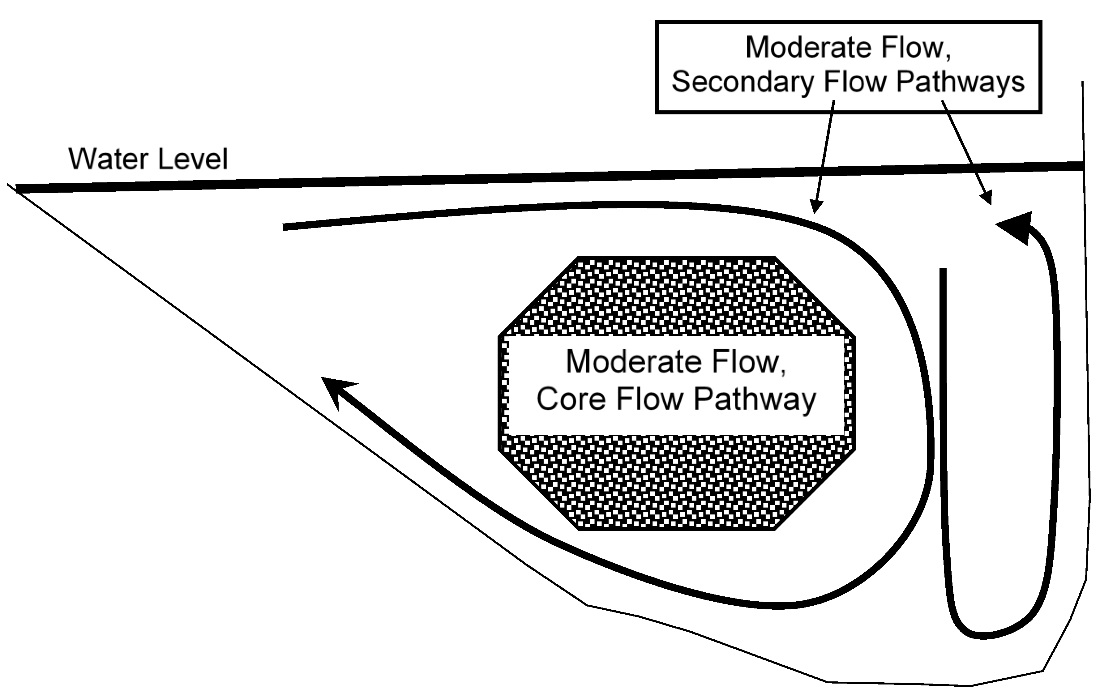
4.9. Integration—The Core Flow Concept

Energy is dissipated on multiple axes as water moves vertically, laterally, and longitudinally along the reach. The LSP of a reach is highly turbulent, with areas of up- and down-welling, though velocities in the downstream direction are depressed. This produces enough flow to keep smaller, more mobile materials in suspension and move these particles toward the point bar or downstream along the outside bank. Burying by sediment load is a perceived threat to freshwater mussels; however, if these hydraulic conditions exist over most mussel bed habitats, burial may not occur frequently (except for bank failure or mass wasting events). This assumes that sediment load has not increased, and discharge has remained relatively consistent over time (i.e., the system is still able to transport its sediment load). Under physical conditions of appropriate depth and channel alignment (curvature), resulting velocities in the LSP over the mussel bed move fine sediments and food items over and away from the bed without reaching levels that entrain and transport mussels and associated substrate, creating the flow refuge.
During low flow, core flow is influenced by the confines of the point bar and directed to the outside bend, where contact with the bank is made at the inflection point. The inflection point is usually toward the middle or upstream portion of the bend [38,60]. Vertical banks were present throughout the reach bend; however, persistent, active erosion indicated by bank failure scars occurred from the middle to the downstream bend limits (i.e., Riffle, Run areas). Vertical banks in the LSP are likely scars of extirpated erosion. Though upstream banks may act as a sediment source, they are likely not a significant source relative to the lower, actively eroding banks. Our observations showed mussel bed downstream limits terminated at or near the point where active erosion appeared, and this likely indicates the point where bedform movement makes conditions unsuitable for mussel habitation.

5. Conclusions

This quasi-experimental observational field study of a large, alluvial, sand-bed-material-dominated river sought to explore, under current river management conditions (e.g., navigation maintenance and upstream flood control), relationships between dynamic freshwater mussel bed habitat under the guise of eco-hydrology [39]. The strategy employed was to select multiple components of the physical habitat energy and material regimes and determine which appear to be most influential in determining mussel habitat with hopes of identifying potential predictors of mussel bed presence or absence. Several factors emerged as important to mussel habitat in the lower White River. First, bed velocity warrants further exploration in terms of strength of flow and direction of flow. Second, bedload appears to be the primary contributor to mussel bed habitat, but additional detailed exploration is needed for core flow pathway and secondary flow pathway interactions. The combined empirical evidence from our observational field study supports the flow refuge concept identified for smaller systems [19] but expands the concept to large non-wadeable streams and includes refuge from sediment transport conditions [37,38]. These characteristics were best expressed in this study through the analysis of mean profile and bed velocity, the Froude number, and bedload transport rates. These variables are valuable for describing current conditions, but to understand why the conditions are present, their relationship with local slope and the channel forming forces of shear stress and stream power should be analyzed with greater resolution. Another influential component of mussel habitat appears to lie in the spatial and temporal dimension and strength of the core and secondary flow pathways, which will likely be highly influenced by the reach horizontal plan distribution and the stream’s geomorphological stage of development. Nevertheless, we make these statements with a caveat that stream habitat conditions are ephemeral (i.e., changing) and that we did not continuously measure hydraulic characteristics, and thereby could have missed important time periods.

Author Contributions

Conceptualization, A.D.C. and J.L.H.; methodology, A.D.C. and A.J.P.; software, A.J.P.; validation, A.D.C. and A.J.P. formal analysis, A.J.P.; investigation, A.J.P, G.M., R.A., R.L., S.S. and W.E.; resources, A.D.C. and J.L.H.; data curation, A.D.C. and A.J.P.; writing—original draft preparation, A.J.P.; writing—review and editing, A.D.C. and J.L.H.; visualization, G.M., R.A., R.L., S.S. and W.E.; supervision, A.J.P.; project administration, A.D.C.; funding acquisition, A.D.C. and J.L.H. All authors have read and agreed to the published version of the manuscript.

Funding

This research was funded by the United States Department of the Interior Fish and Wildlife Service under Grant Agreement No. 401813G077.

Acknowledgments

Special thanks to J. Krystofik of the Arkansas Field Office of the Fish and Wildlife Service for being an advocate of this project. We thank R. Fokidis, H. McIntyre, and J. Shoemaker for their assistance with field and laboratory work. We also thank S. Haas and M. Hanley of the Arkansas Chapter of The Nature Conservancy for initial consultations regarding field conditions and methodologies and D. Peck for analytical insight and guidance. Early versions of this manuscript were reviewed by S.E. Trauth and R.L. Johnson of Arkansas State University. This paper benefited from edits and comments provided by three anonymous reviewers.

Conflicts of Interest

The authors declare no conflict of interest.

Appendix A

Table A1. Pooled mean velocity (m·s−1; ±SD) by lateral position (Inside, Middle, Outside) across seasons (Spring, Autumn, Winter), regions (Middle, Lower), bed type (Current, Extirpated), and habitat (Riffle, LSP, Glide).
SeasonRegionBed TypeHabitatLateral Position
Inside (±SD)Middle (±SD)Outside (±SD)
SpringMiddleCurrentRiffle0.68 (0.15)0.68 (0.18)0.34 (0.12)
LSP0.66 (0.16)0.66 (0.11)0.38 (0.07)
Glide0.55 (0.19)0.82 (0.13)0.84 (0.27)
MiddleExtirpatedRiffle0.61 (0.10)0.78 (0.19)0.64 (0.22)
LSP0.66 (0.18)0.66 (0.16)0.62 (0.22)
Glide0.45 (0.25)0.70 (0.20)0.79 (0.21)
LowerCurrentRiffle0.85 (0.11)0.84 (0.11)0.53 (0.31)
LSP0.73 (0.12)0.83 (0.08)0.67 (0.11)
Glide0.53 (0.17)0.98 (0.03)1.01 (0.05)
LowerExtirpatedRiffle0.74 (0.18)0.88 (0.15)0.69 (0.10)
LSP0.61 (0.02)0.84 (0.11)0.72 (0.05)
Glide0.58 (0.06)0.81 (0.23)0.89 (0.08)
AutumnMiddleCurrentRiffle0.55 (0.16)0.66 (0.16)0.41 (0.13)
LSP0.55 (0.26)0.65 (0.13)0.41 (0.14)
Glide0.26 (0.18)0.50 (0.06)0.60 (0.09)
MiddleExtirpatedRiffle0.65 (0.28)0.68 (0.08)0.40 (0.07)
LSP0.45 (0.25)0.59 (0.10)0.50 (0.27)
Glide0.25 (0.10)0.72 (0.06)0.71 (0.27)
LowerCurrentRiffle0.87 (0.15)0.88 (0.20)0.58 (0.21)
LSP0.76 (0.26)0.80 (0.22)0.62 (0.26)
Glide0.63 (0.13)0.86 (0.20)0.77 (0.13)
LowerExtirpatedRiffle0.96 (0.31)0.90 (0.25)0.94 (0.29)
LSP0.71 (0.37)0.91 (0.27)0.62 (0.15)
Glide0.53 (0.31)0.71 (0.29)0.86 (0.21)
WinterMiddleCurrentRiffle1.08 (0.09)1.02 (0.10)0.74 (0.11)
LSP1.04 (0.20)1.01 (0.08)0.51 (0.07)
Glide0.67 (0.28)1.14 (0.07)1.20 (0.13)
MiddleExtirpatedRiffle1.01 (0.21)1.06 (0.11)0.83 (0.12)
LSP0.98 (0.14)1.07 (0.11)0.68 (0.22)
Glide0.80 (0.10)1.17 (0.06)1.24 (0.11)
LowerCurrentRiffle1.10 (0.09)0.99 (0.08)0.77 (0.12)
LSP1.04 (0.11)0.99 (0.05)0.70 (0.18)
Glide0.32 (0.51)1.02 (0.06)1.27 (0.22)
LowerExtirpatedRiffle1.01 (0.14)0.97 (0.18)0.85 (0.22)
LSP0.75 (0.11)0.92 (0.14)0.65 (0.17)
Glide0.60 (0.13)0.90 (0.08)1.00 (0.01)
Table A2. Pooled cell mean estimated bed velocity (m·s−1; ±SD) by lateral position (Inside, Middle, Outside) across seasons (Spring, Autumn, Winter), regions (Middle, Lower), bed type (Current, Extirpated), and habitat (Riffle, LSP, Glide).
SeasonRegionBed TypeHabitatLateral Position
Inside (±SD)Middle (±SD)Outside (±SD)
SpringMiddleCurrentRiffle0.47 (0.10)0.47 (0.13)0.23 (0.08)
LSP0.47 (0.11)0.46 (0.07)0.26 (0.05)
Glide0.39 (0.13)0.58 (0.09)0.58 (0.19)
MiddleExtirpatedRiffle0.43 (0.07)0.55 (0.13)0.45 (0.16)
LSP0.46 (0.12)0.46 (0.11)0.43 (0.15)
Glide0.31 (0.18)0.49 (0.14)0.55 (0.14)
LowerCurrentRiffle0.59 (0.07)0.59 (0.08)0.37 (0.22)
LSP0.51 (0.08)0.58 (0.06)0.47 (0.07)
Glide0.37 (0.12)0.68 (0.02)0.71 (0.03)
LowerExtirpatedRiffle0.52 (0.12)0.61 (0.11)0.48 (0.07)
LSP0.42 (0.01)0.59 (0.08)0.50 (0.03)
Glide0.41 (0.05)0.57 (0.17)0.62 (0.05)
AutumnMiddleCurrentRiffle0.38 (0.11)0.46 (0.12)0.29 (0.09)
LSP0.38 (0.18)0.46 (0.09)0.29 (0.11)
Glide0.18 (0.13)0.34 (0.05)0.41 (0.07)
MiddleExtirpatedRiffle0.45 (0.20)0.47 (0.06)0.28 (0.05)
LSP0.31 (0.18)0.41 (0.07)0.35 (0.19)
Glide0.17 (0.07)0.51 (0.04)0.50 (0.18)
LowerCurrentRiffle0.61 (0.10)0.61 (0.14)0.40 (0.15)
LSP0.53 (0.18)0.56 (0.15)0.44 (0.18)
Glide0.44 (0.09)0.60 (0.14)0.53 (0.09)
LowerExtirpatedRiffle0.67 (0.21)0.62 (0.18)0.66 (0.20)
LSP0.50 (0.26)0.64 (0.19)0.44 (0.10)
Glide0.37 (0.22)0.50 (0.20)0.60 (0.25)
WinterMiddleCurrentRiffle0.76 (0.06)0.72 (0.07)0.52 (0.07)
LSP0.73 (0.13)0.72 (0.07)0.36 (0.05)
Glide0.47 (0.20)0.80 (0.05)0.84 (0.09)
MiddleExtirpatedRiffle0.70 (0.15)0.74 (0.07)0.58 (0.08)
LSP0.69 (0.11)0.75 (0.08)0.47 (0.16)
Glide0.56 (0.07)0.82 (0.05)0.87 (0.08)
LowerCurrentRiffle0.77 (0.06)0.69 (0.05)0.54 (0.08)
LSP0.73 (0.07)0.69 (0.03)0.49 (0.13)
Glide0.23 (0.36)0.71 (0.05)0.89 (0.15)
LowerExtirpatedRiffle0.71 (0.10)0.68 (0.13)0.60 (0.16)
LSP0.52 (0.08)0.64 (0.10)0.45 (0.12)
Glide0.42 (0.09)0.63 (0.06)0.70 (0.01)
Table A3. Pooled mean cell Froude numbers (±SD) by lateral position (Inside, Middle, Outside) across seasons (Spring, Autumn, Winter), regions (Middle, Lower), bed type (Current, Extirpated), and habitat (Riffle, LSP, Glide).
SeasonRegionBed TypeHabitatLateral Position
Inside (±SD)Middle (±SD)Outside (±SD)
SpringMiddleCurrentRiffle0.10 (0.02)0.09 (0.03)0.06 (0.04)
LSP0.09 (0.02)0.08 (0.01)0.05 (0.02)
Glide0.10 (0.06)0.12 (0.03)0.10 (0.04)
MiddleExtirpatedRiffle0.09 (0.03)0.10 (0.02)0.09 (0.02)
LSP0.10 (0.01)0.08 (0.02)0.07 (0.03)
Glide0.08 (0.04)0.09 (0.03)0.08 (0.03)
LowerCurrentRiffle0.11 (0.02)0.11 (0.01)0.07 (0.04)
LSP0.16 (0.05)0.11 (0.02)0.06 (0.01)
Glide0.09 (0.03)0.13 (0.01)0.12 (0.01)
LowerExtirpatedRiffle0.10 (0.02)0.11 (0.02)0.08 (0.01)
LSP0.10 (0.01)0.11 (0.01)0.08 (0.01)
Glide0.10 (0.02)0.11 (0.03)0.11 (0.03)
AutumnMiddleCurrentRiffle0.09 (0.04)0.11 (0.04)0.07 (0.03)
LSP0.12 (0.06)0.11 (0.03)0.06 (0.03)
Glide0.06 (0.05)0.08 (0.02)0.08 (0.02)
MiddleExtirpatedRiffle0.11 (0.03)0.12 (0.02)0.06 (0.02)
LSP0.10 (0.05)0.10 (0.02)0.06 (0.03)
Glide0.07 (0.05)0.11 (0.03)0.09 (0.05)
LowerCurrentRiffle0.14 (0.04)0.15 (0.04)0.09 (0.03)
LSP0.20 (0.06)0.14 (0.05)0.08 (0.04)
Glide0.13 (0.07)0.14 (0.04)0.11 (0.03)
LowerExtirpatedRiffle0.17 (0.05)0.15 (0.04)0.15 (0.06)
LSP0.16 (0.09)0.16 (0.04)0.09 (0.03)
Glide0.12 (0.05)0.12 (0.05)0.12 (0.03)
WinterMiddleCurrentRiffle0.12 (0.01)0.11 (0.02)0.08 (0.01)
LSP0.13 (0.03)0.11 (0.01)0.05 (0.01)
Glide0.09 (0.03)0.12 (0.01)0.11 (0.01)
MiddleExtirpatedRiffle0.11 (0.02)0.12 (0.01)0.09 (0.01)
LSP0.12 (0.01)0.12 (0.01)0.06 (0.02)
Glide0.12 (0.01)0.12 (0.02)0.12 (0.02)
LowerCurrentRiffle0.12 (0.02)0.10 (0.01)0.08 (0.02)
LSP0.15 (0.03)0.11 (0.00)0.07 (0.02)
Glide0.04 (0.06)0.11 (0.01)0.12 (0.02)
LowerExtirpatedRiffle0.12 (0.02)0.11 (0.02)0.09 (0.02)
LSP0.09 (0.01)0.10 (0.02)0.07 (0.02)
Glide0.08 (0.02)0.10 (0.01)0.11 (0.01)
Table A4. Pooled mean shear stress (N/ms) (±SD) by lateral position (Inside, Middle, Outside) across seasons (Spring, Autumn, Winter), regions (Middle, Lower), bed type (Current, Extirpated), and habitat (Riffle, LSP, Glide).
SeasonRegionBed TypeHabitatLateral Position
Inside (±SD)Middle (±SD)Outside (±SD)
SpringMiddleCurrentRiffle7.26 (3.93)5.57 (4.07)8.01 (7.50)
LSP6.41 (3.37)1.50 (2.14)4.06 (5.86)
Glide1.22 (1.21)3.23 (4.85)10.42 (10.16)
MiddleExtirpatedRiffle6.83 (10.42)12.24 (13.35)8.34 (7.12)
LSP12.22 (5.89)5.00 (2.02)3.10 (3.28)
Glide17.90 (17.85)12.68 (7.89)12.96 (7.35)
LowerCurrentRiffle4.64 (4.05)6.83 (5.84)2.72 (3.74)
LSP11.59 (7.03)8.81 (10.36)9.69 (8.76)
Glide10.96 (14.63)4.07 (3.35)11.07 (15.06)
LowerExtirpatedRiffle4.72 (6.94)7.34 (6.45)6.78 (7.69)
LSP8.22 (7.09)5.37 (6.76)6.59 (5.97)
Glide10.05 (7.43)6.88 (11.60)13.91 (3.13)
AutumnMiddleCurrentRiffle7.03 (1.40)11.67 (14.08)11.37 (14.44)
LSP2.80 (1.67)5.23 (5.63)10.78 (10.12)
Glide79.78 (117.15)17.19 (13.62)20.97 (7.29)
MiddleExtirpatedRiffle36.36 (33.23)37.57 (51.45)32.53 (19.32)
LSP14.72 (8.85)12.92 (19.63)13.98 (19.90)
Glide46.16 (69.37)5.00 (7.42)16.15 (14.04)
LowerCurrentRiffle22.46 (22.26)8.17 (7.88)19.00 (3.18)
LSP25.28 (15.29)30.44 (14.42)18.65 (16.16)
Glide31.95 (32.40)3.67 (5.08)19.33 (9.27)
LowerExtirpatedRiffle74.33 (52.90)13.70 (13.95)8.65 (11.83)
LSP53.80 (16.14)14.35 (11.65)22.49 (26.29)
Glide114.58 (112.12)8.79 (8.49)14.59 (16.39)
WinterMiddleCurrentRiffle13.64 (1.36)12.16 (4.85)15.52 (14.34)
LSP1.94 (3.06)6.32 (3.65)10.19 (8.81)
Glide7.27 (6.22)7.24 (4.74)5.95 (5.79)
MiddleExtirpatedRiffle25.41 (20.88)12.79 (10.71)8.16 (4.08)
LSP9.64 (9.03)16.72 (13.84)7.43 (11.82)
Glide6.33 (6.13)4.17 (1.45)2.03 (1.94)
LowerCurrentRiffle4.08 (2.48)4.88 (5.30)5.99 (2.60)
LSP2.08 (2.53)5.28 (1.43)2.79 (2.26)
Glide0.35 (0.51)7.72 (4.66)1.15 (1.49)
LowerExtirpatedRiffle11.38 (1.23)9.68 (7.15)11.60 (1.67)
LSP2.82 (2.24)10.58 (10.51)5.74 (6.35)
Glide5.17 (6.39)10.65 (2.30)11.12 (11.17)
Table A5. Pooled mean stream power (W/m) (±SD) by lateral position (Inside, Middle, Outside) across seasons (Spring, Autumn, Winter), regions (Middle, Lower), bed type (Current, Extirpated), and habitat (Riffle, LSP, Glide).
SeasonRegionBed TypeHabitatLateral Position
Inside (±SD)Middle (±SD)Outside (±SD)
SpringMiddleCurrentRiffle4.90 (3.02)4.04 (3.83)2.82 (3.19)
LSP3.96 (1.74)1.11 (1.63)1.78 (2.63)
Glide0.80 (0.78)2.76 (4.10)6.87 (4.14)
MiddleExtirpatedRiffle4.69 (7.30)8.67 (8.03)5.49 (5.95)
LSP8.67 (5.43)3.54 (1.95)1.95 (1.84)
Glide7.86 (6.69)8.23 (3.65)9.72 (5.60)
LowerCurrentRiffle4.06 (3.45)6.18 (5.61)0.69 (0.66)
LSP8.14 (3.28)6.71 (7.56)6.16 (8.05)
Glide5.37 (6.72)4.04 (3.33)11.45 (15.77)
LowerExtirpatedRiffle2.89 (3.92)5.82 (4.72)4.43 (4.88)
LSP4.96 (4.26)4.09 (4.74)4.90 (4.54)
Glide6.02 (4.92)4.60 (7.63)12.45 (3.35)
AutumnMiddleCurrentRiffle3.84 (1.32)8.28 (10.87)4.55 (6.17)
LSP1.48 (1.28)3.65 (4.42)3.87 (2.66)
Glide26.13 (39.81)8.73 (7.50)12.02 (2.24)
MiddleExtirpatedRiffle18.79 (14.50)23.72 (32.57)13.81 (9.18)
LSP5.73 (4.76)6.83 (10.04)5.81 (8.44)
Glide10.61 (14.93)3.31 (4.81)11.26 (10.81)
LowerCurrentRiffle19.25 (18.67)6.08 (4.49)10.86 (4.00)
LSP17.76 (8.02)26.73 (18.14)15.13 (17.51)
Glide22.77 (24.68)3.64 (5.14)14.51 (5.87)
LowerExtirpatedRiffle49.50 (41.37)10.49 (8.63)7.87 (11.44)
LSP34.23 (11.58)14.42 (12.06)13.77 (17.35)
Glide37.67 (32.59)6.33 (5.49)14.61 (18.89)
WinterMiddleCurrentRiffle14.84 (2.45)12.10 (3.56)11.93 (11.89)
LSP2.18 (3.47)6.20 (3.29)4.87 (3.75)
Glide3.73 (1.25)8.35 (5.50)10.42 (3.26)
MiddleExtirpatedRiffle23.09 (14.44)14.13 (12.41)6.46 (2.49)
LSP9.72 (9.24)18.84 (16.73)5.67 (9.32)
Glide4.77 (4.11)4.93 (1.84)2.38 (2.21)
LowerCurrentRiffle4.51 (2.88)4.89 (5.59)4.63 (2.21)
LSP2.28 (2.92)5.21 (1.39)2.05 (2.08)
Glide0.29 (0.49)8.02 (5.25)1.56 (2.07)
LowerExtirpatedRiffle11.48 (1.04)8.99 (6.64)9.84 (3.09)
LSP2.10 (1.60)8.90 (8.12)3.02 (2.75)
Glide3.3. (4.96)9.66 (2.74)11.10 (11.10)
Table A6. Mean bedload discharge (g·s−1) (±SD) by lateral position (Inside, Middle, Outside) across seasons (Spring, Autumn, Winter), regions (Middle, Lower), bed type (Current, Extirpated), and habitat (Riffle, LSP, Glide).
SeasonRegionBed TypeHabitatLateral Position
Inner (±SD)Middle (±SD)Outer (±SD)
SpringMiddleCurrentRiffle114.60 (67.47)848.03 (1138.40)28.37 (45.67
LSP446.97 (691.48)85.30 (112.79)9.43 (15.65)
Glide6.03 (9.26)86.60 (67.74)120.33 (108.23)
MiddleExtirpatedRiffle73.27 (112.70)665.13 (555.18)115.30 (121.16)
LSP206.07 (225.97)48.63 (35.68)9.77 (2.27)
Glide159.40 (272.46)45.30 (27.74)2.43 (2.56)
LowerCurrentRiffle636.50 (138.23)438.73 (726.92)3.33 (3.57)
LSP537.80 (580.15)489.63 (376.00)11.70 (18.48)
Glide16.83 (21.40)385.00 (75.10)503.97 (716.04)
LowerExtirpatedRiffle76.5 (114.60)181.83 (237.15)22.30 (26.07)
LSP342.87 (296.95)776.37 (525.85)2.47 (2.73)
Glide32.83 (43.87)573.47 (199.21)493.60 (600.19)
AutumnMiddleCurrentRiffle358.53 (342.05)381.40 (583.05)255.10 (417.80)
LSP249.13 (205.32)107.10 (93.21)53.70 (74.37)
Glide0.80 (0.75)65.33 (39.25)82.13 (141.05)
MiddleExtirpatedRiffle366.23 (573.28)150.77 (166.96)75.10 (83.03)
LSP496.07 (857.48)364.87 (375.87)1.77 (1.12)
Glide0.07 (0.12)652.40 (797.53)49.50 (82.80)
LowerCurrentRiffle1112.83 (1452.10)153.77 (107.48)12.77 (19.17)
LSP4.63 (1.69)711.87 (706.91)3.57 (3.94)
Glide13.37 (13.12)1300.43 (2073.32)114.53 (122.80)
LowerExtirpatedRiffle74.47 (49.43)370.27 (426.88)128.8 (135.14)
LSP257.47 (11.83)154.1 (221.43)8.67 (15.01)
Glide7.6 (8.6)45.27 (42.57)669.2 (1004.66)
WinterMiddleCurrentRiffle159.50 (56.88)216.93 (183.47)53.93 (75.33)
LSP862.23 (741.18)595.17 (382.97)190.73 (283.19)
Glide224.63 (231.50)116.10 (146.32)76.57 (23.53)
MiddleExtirpatedRiffle599.73 (589.24)395.03 (167.88)154.80 (36.85)
LSP820.70 (791.63)374.13 (109.73)2.30 (0.80)
Glide424.90 (289.27)146.33 (115.34)620.10 (938.07)
LowerCurrentRiffle201.77 (215.14)227.63 (212.27)169.53 (122.17)
LSP2219.77 (2859.16)129.7 (99.30)18.47 (31.64)
Glide13.60 (17.84)206.47 (86.90)268.33 (464.77)
LowerExtirpatedRiffle115.67 (73.64)404.00 (390.96)33.20 (23.90)
LSP1218.00 (1872.08)338.23 (404.08)58.50 (58.10)
Glide305.47 (263.08)90.5 (83.15)302.03 (273.79)
Table A7. Pooled mean particle size (mm) (±SD) by lateral position (Inside, Middle, Outside) across seasons (Spring, Autumn, Winter), regions (Middle, Lower), bed type (Current, Extirpated), and habitat (Riffle, LSP, Glide).
SeasonRegionBed TypeHabitatLateral Position
Inner (±SD)Middle (±SD)Outer (±SD)
SpringMiddleCurrentRiffle0.48 (0.06)0.20 (0.17)0.69 (0.31)
LSP0.51 (0.03)0.32 (0.02)0.56 (0.15)
Glide0.51 (0.60)0.35 (0.03)0.20 (0.35)
MiddleExtirpatedRiffle0.52 (0.23)0.38 (0.06)0.38 (0.07)
LSP0.44 (0.13)0.35 (0.05)0.41 (0.10)
Glide0.72 (0.23)0.39 (0.07)0.33 (0.29)
LowerCurrentRiffle0.59 (0.09)0.39 (0.11)0.19 (0.17)
LSP0.43 (0.09)0.41 (0.08)0.61 (0.63)
Glide0.53 (0.45)0.34 (0.01)0.41 (0.42)
LowerExtirpatedRiffle0.60 (0.34)0.30 (0.03)0.35 (0.03)
LSP0.32 (0.30)0.33 (0.00)0.48 (0.42)
Glide0.33 (0.08)0.43 (0.15)0.71 (0.20)
AutumnMiddleCurrentRiffle0.38 (0.06)0.26 (0.05)0.34 (0.12)
LSP0.65 (0.31)0.30 (0.01)0.53 (0.37)
Glide0.13 (0.14)0.37 (0.06)0.32 (0.55)
MiddleExtirpatedRiffle0.60 (0.24)0.41 (0.08)0.31 (0.03)
LSP0.47 (0.48)0.35 (0.06)0.36 (0.22)
Glide0.25 (0.44)0.43 (0.03)0.68 (0.25)
LowerCurrentRiffle0.30 (0.29)0.31 (0.03)0.30 (0.10)
LSP0.35 (0.03)0.38 (0.14)0.59 (0.51)
Glide0.46 (0.29)0.32 (0.01)0.44 (0.50)
LowerExtirpatedRiffle0.32 (0.07)0.30 (0.02)0.30 (0.05)
LSP0.28 (0.24)0.32 (0.02)0.23 (0.21)
Glide0.41 (0.17)0.30 (0.04)0.50 (0.14)
WinterMiddleCurrentRiffle0.38 (0.06)0.31 (0.02)0.36 (0.10)
LSP0.48 (0.13)0.32 (0.06)0.32 (0.06)
Glide0.39 (0.21)0.42 (0.10)0.80 (0.40)
MiddleExtirpatedRiffle0.45 (0.12)0.39 (0.08)0.38 (0.11)
LSP0.49 (0.13)0.32 (0.04)0.48 (0.17)
Glide0.28 (0.06)0.35 (0.03)0.56 (0.17)
LowerCurrentRiffle0.36 (0.07)0.30 (0.08)0.38 (0.14)
LSP0.40 (0.07)0.41 (0.12)0.40 (0.45)
Glide0.20 (0.17)0.32 (0.01)0.18 (0.32)
LowerExtirpatedRiffle0.46 (0.04)0.31 (0.02)0.37 (0.14)
LSP0.50 (0.12)0.33 (0.01)0.23 (0.20)
Glide0.35 (0.02)0.33 (0.02)0.51 (0.07)

References

  1. Southwood, T.R.E. Tactics, Strategies and Templets. Oikos 1988, 52, 3–18. [Google Scholar] [CrossRef]
  2. Scarsbrook, M.R.; Townsend, C.R. Stream Community Structure in Relation to Spatial and Temporal Variation: A Habitat Templet Study of Two Contrasting New Zealand Streams. Freshw. Biol. 1993, 29, 395–410. [Google Scholar] [CrossRef]
  3. Townsend, C.R.; Hildrew, A.G. Species Traits in Relation to a Habitat Templet for River Systems. Freshw. Biol. 1994, 31, 265–275. [Google Scholar] [CrossRef]
  4. Frissell, C.A.; Liss, W.J.; Warren, C.E.; Hurley, M.D. A Hierarchical Framework for Stream Habitat Classification: Viewing Streams in a Watershed Context. Environ. Manag. 1986, 10, 199–214. [Google Scholar] [CrossRef]
  5. Poff, N.L. Landscape Filters and Species Traits: Towards Mechanistic Understanding and Prediction in Stream Ecology. J. N. Am. Benthol. Soc. 1997, 16, 391–409. [Google Scholar] [CrossRef]
  6. Neves, R.J. A State-of-the-Unionids Address. In Conservation and Management of Freshwater Mussels, Proceedings of a UMRCC Symposium, St. Louis, MO, USA, 12–14 October 1992; Cummings, K.S., Buchanan, A.C., Koch, L.M., Eds.; Upper Mississippi River Conservation Committee: Rock Island, IL, USA, 1993; pp. 1–10. [Google Scholar]
  7. Freshwater Mollusk Conservation Society. A National Strategy for the Conservation of Native Freshwater Mollusks. Freshw. Mollusk Biol. Conserv. 2016, 19, 1–21. [Google Scholar] [CrossRef]
  8. Vannote, R.L.; Minshall, G.W. Fluvial Processes and Local Lithology Controlling Abundance, Structure, and Composition of Mussel Beds. Proc. Natl. Acad. Sci. USA 1982, 79, 4103–4107. [Google Scholar] [CrossRef] [Green Version]
  9. Strayer, D.L. The Effects of Surface Geology and Stream Size on Freshwater Mussel (Bivalvia, Unionidae) Distribution in Southeastern Michigan, USA. Freshw. Biol. 1983, 13, 253–264. [Google Scholar] [CrossRef]
  10. Neves, R.J.; Widlak, J.C. Habitat Ecology of Juvenile Freshwater Mussels (Bivalvia: Unionidae) in a Headwater Stream in Virginia. Am. Malacol. Bull. 1987, 5, 1–7. [Google Scholar]
  11. Bailey, R. Habitat Selection by a Freshwater Mussel: An Experimental Test. Malacologia 1989, 31, 205–210. [Google Scholar]
  12. Way, C.M.; Miller, A.C.; Payne, B.S. The Influence of Physical Factors on the Distribution and Abundance of Freshwater Mussels (Bivalvia: Unionidae) in the Lower Tennessee River. Nautilus 1989, 103, 96–98. [Google Scholar]
  13. Holland-Bartels, L.E. Physical Factors and Their Influence on the Mussel Fauna of a Main Channel Border Habitat of the Upper Mississippi River. J. N. Am. Benthol. Soc. 1990, 9, 327–335. [Google Scholar] [CrossRef]
  14. Strayer, D.L. Macrohabitats of Freshwater Mussels (Bivalvia: Unionacea) in Streams of the Northern Atlantic Slope. J. N. Am. Benthol. Soc. 1993, 12, 236–246. [Google Scholar] [CrossRef]
  15. Strayer, D.L.; Ralley, J. Microhabitat Use by an Assemblage of Stream-Dwelling Unionaceans (Bivalvia), Including Two Rare Species of Alasmidonta. J. N. Am. Benthol. Soc. 1993, 12, 247–258. [Google Scholar] [CrossRef]
  16. Di Maio, J.; Corkum, L.D. Relationship between the Spatial Distribution of Freshwater Mussels (Bivalvia: Unionidae) and the Hydrological Variability of Rivers. Can. J. Zool. 1995, 15, 663–671. [Google Scholar] [CrossRef]
  17. Di Maio, J.; Corkum, L.D. Patterns of Orientation in Unionids as a Function of Rivers with Differing Hydrological Variability. J. Molluscan Stud. 1997, 63, 531–539. [Google Scholar] [CrossRef]
  18. Brim-Box, J.B.; Mossa, J. Sediment, Land Use, and Freshwater Mussels: Prospects and Problems. J. N. Am. Benthol. Soc. 1999, 18, 99–117. [Google Scholar]
  19. Strayer, D.L. Use of Flow Refuges by Unionid Mussels in Rivers. J. N. Am. Benthol. Soc. 1999, 18, 468–476. [Google Scholar] [CrossRef]
  20. Hastie, L.C.; Young, M.R.; Boon, P.J. Growth Characteristics of Freshwater Pearl Mussels, Margaritifera margaritifera (L.). Freshw. Biol. 2000, 43, 243–256. [Google Scholar] [CrossRef]
  21. Hardison, B.S.; Layzer, J.B. Relations between Complex Hydraulics and the Localized Distribution of Mussels in Three Regulated Rivers. Regul. Rivers Res. Manag. Int. J. Devoted River Res. Manag. 2001, 17, 77–84. [Google Scholar] [CrossRef]
  22. Arbuckle, K.E.; Downing, J.A. The Influence of Watershed Land Use on Lake N:P in a Predominantly Agricultural Landscape. Limnol. Oceanogr. 2001, 46, 970–975. [Google Scholar] [CrossRef]
  23. Brim-Box, J.; Dorazio, R.M.; Liddell, W.D. Relationships between Streambed Substrate Characteristics and Freshwater Mussels (Bivalvia: Unionidae) in Coastal Plain Streams. J. N. Am. Benthol. Soc. 2002, 21, 253–260. [Google Scholar]
  24. Poole, K.E.; Downing, J.A. Relationship of Declining Mussel Biodiversity to Stream-Reach and Watershed Characteristics in an Agricultural Landscape. J. N. Am. Benthol. Soc. 2004, 23, 114–125. [Google Scholar] [CrossRef]
  25. Morales, Y.; Weber, L.; Mynett, A.; Newton, T. Effects of Substrate and Hydrodynamic Conditions on the Formation of Mussel Beds in a Large River. J. N. Am. Benthol. Soc. 2006, 25, 664–676. [Google Scholar] [CrossRef] [Green Version]
  26. Newton, T.J.; Woolnough, D.A.; Strayer, D.L. Using Landscape Ecology to Understand and Manage Freshwater Mussel Populations. J. N. Am. Benthol. Soc. 2008, 27, 424–439. [Google Scholar] [CrossRef]
  27. Allen, D.C.; Vaughn, C.C. Complex Hydraulic and Substrate Variables Limit Freshwater Mussel Species Richness and Abundance. J. N. Am. Benthol. Soc. 2010, 29, 383–394. [Google Scholar] [CrossRef]
  28. Maloney, K.O.; Lellis, W.A.; Bennett, R.M.; Waddle, T.J. Habitat Persistence for Sedentary Organisms in Managed Rivers: The Case for the Federally Endangered Dwarf Wedgemussel (Alasmidonta heterodon) in the Delaware River. Freshw. Biol. 2012, 57, 1315–1327. [Google Scholar] [CrossRef]
  29. Hornbach, D.J. Macrohabitat Factors Influencing the Distribution of Naiads in the St. Croix River, Minnesota and Wisconsin, USA. In Ecology and Evolution of the Freshwater Mussels Unionoida; Springer: Berlin, Germany, 2001; pp. 213–230. [Google Scholar]
  30. Gangloff, M.; Feminella, J. Stream Channel Geomorphology Influences Mussel Abundance in Southern Appalachian Streams, USA. Freshw. Biol. 2007, 52, 64–74. [Google Scholar] [CrossRef]
  31. Steuer, J.J.; Newton, T.J.; Zigler, S.J. Use of Complex Hydraulic Variables to Predict the Distribution and Density of Unionids in a Side Channel of the Upper Mississippi River. Hydrobiologia 2008, 610, 67–82. [Google Scholar] [CrossRef]
  32. Zigler, S.J.; Newton, T.J.; Steuer, J.J.; Bartsch, M.R.; Sauer, J.S. Importance of Physical and Hydraulic Characteristics to Unionid Mussels: A Retrospective Analysis in a Reach of Large River. Hydrobiologia 2008, 598, 343–360. [Google Scholar] [CrossRef]
  33. Daraio, J.A.; Weber, L.J.; Newton, T.J. Hydrodynamic Modeling of Juvenile Mussel Dispersal in a Large River: The Potential Effects of Bed Shear Stress and Other Parameters. J. N. Am. Benthol. Soc. 2010, 29, 838–851. [Google Scholar] [CrossRef]
  34. Daraio, J.A.; Weber, L.J.; Newton, T.J.; Nestler, J.M. A Methodological Framework for Integrating Computational Fluid Dynamics and Ecological Models Applied to Juvenile Freshwater Mussel Dispersal in the Upper Mississippi River. Ecol. Model. 2010, 221, 201–214. [Google Scholar] [CrossRef]
  35. Smit, R.; Kaeser, A. Defining Freshwater Mussel Mesohabitat Associations in an Alluvial, Coastal Plain River. Freshw. Sci. 2016, 35, 1276–1290. [Google Scholar] [CrossRef]
  36. Christian, A.D.; Harris, J.L.; Posey, W.R.; Hockmuth, J.F.; Harp, G.L. Freshwater Mussel (Bivalvia: Unionidae) Assemblages of the Lower Cache River, Arkansas. Southeast. Nat. 2005, 4, 487–512. [Google Scholar] [CrossRef]
  37. Bathurst, J.C.; Hey, R.D.; Thorne, C.R. Secondary Flow and Shear Stress at River Bends. J. Hydraul. Div. 1979, 105, 1277–1295. [Google Scholar]
  38. Bathurst, J. Environmental River Flow Hydraulics. In Applied Fluvial Geomorphology for River Engineering and Management; John Wiley & Sons, Inc.: New York, NY, USA, 1997; pp. 69–93. [Google Scholar]
  39. Statzner, R. Growth and Reynolds Number of Lotic Macroinvertebrates: A Problem for Adaptation of Shape to Drag. Oikos 1988, 51, 84–87. [Google Scholar] [CrossRef]
  40. Gordon, M.E. Mollusca of the White River, Arkansas and Missouri. Southwest. Nat. 1982, 27, 347–352. [Google Scholar] [CrossRef]
  41. Coker, R.E. Fresh-Water Mussels and Mussel Industries of the United States; US Government Printing Office: Washington, DC, WA, USA, 1919.
  42. Williams, J.D.; Warren, M.L.; Cummings, K.S.; Harris, J.L.; Neves, R.J. Conservation Status of Freshwater Mussels of the United States and Canada. Fisheries 1993, 18, 6–22. [Google Scholar] [CrossRef]
  43. Harris, J.L.; Posey, W.R., II; Davidson, C.L.; Farris, J.L.; Oetker, S.R.; Stoeckel, J.N.; Crump, B.G.; Barnett, M.S.; Martin, H.C.; Matthews, M.W.; et al. Unionoida (Mollusca: Margaritiferidae, Unionidae) in Arkansas, Third Status Review. J. Ark. Acad. Sci. 2009, 63, 50–84. [Google Scholar]
  44. Christian, A.D. Analysis of the Commercial Mussel Beds in the Cache and White Rivers in Arkansas. Master’s Thesis, Arkansas State University, Jonesboro, AR, USA, 1995. [Google Scholar]
  45. Christian, A.D.; Harris, J.L. Development and Assessment of a Sampling Design for Mussel Assemblages in Large Streams. Am. Midl. Nat. 2005, 153, 284–292. [Google Scholar] [CrossRef]
  46. Harris, J.L.; Christian, A.D. Current Status of the Freshwater Mussel Fauana of the White River, Arkansas, River Miles 10-255; Report; U.S Army Corps of Engineers: Memphis, TN, USA, 2000.
  47. United States Geological Survey, USGS Stream Stats. Available online: https://streamstats.usgs.gov/ss/ (accessed on 6 March 2018).
  48. U.S. Department of Agriculture: Forest Service. Ozark-Ouachita Highlands Assessment: Aquatic Conditions; Report 3 of 5 General Technical Report SRS-33; U.S. Department of Agriculture, Forest Service, Southern Research Station: Asheville, CA, USA, 1999.
  49. Bisson, P.A.; Nielsen, J.L.; Palmason, R.A.; Grove, L.E. A System of Naming Habitat in Small Streams, with Examples of Habitat Utilization by Salmonids during Low Streamflow. In Proceedings of the Symposium on Acquisition and Utilization of Aquatic Habitat Inventory Information, Portland, OR, USA, 28–30 October 1981; Armantrout, N.B., Ed.; Hagen Publishing Company: Los Angeles, CA, USA, 1982; pp. 62–73. [Google Scholar]
  50. Gordon, N.D.; McMahon, T.A.; Finlayson, B.L.; Gippel, C.; Nathan, R.J. Stream Hydrology: An Introduction for Ecologists, 2nd ed.; John Wiley & Sons Ltd.: West Sussex, UK, 2004. [Google Scholar]
  51. United States Army Corps of Engineers Memphis District. White River Gauges. Available online: http://www.mvm.usace.army.mil/hydraulics/docs/white.htm (accessed on 15 January 2005).
  52. Rempel, L.L.; Richardson, J.S.; Healey, M.C. Macroinvertebrate Community Structure along Gradients of Hydraulic and Sedimentary Conditions in a Large Gravel-bed River. Freshw. Biol. 2000, 45, 57–73. [Google Scholar] [CrossRef]
  53. Das, B.M. Soil Mechanics Laboratory Manual; Engineering Press: Austin, TX, USA, 1997. [Google Scholar]
  54. Peck, A.J. A Reach Scale Comparison of Fluvial Geomorphological Conditions between Current and Historic Freshwater Mussel Beds in the White River, Arkansas. Master’s Thesis, Arkansas State University, Jonesboro, AR, USA, 2005. [Google Scholar]
  55. Lessios, H.A. Testing Electrophoretic Data for Agreement with Hardy-Weinberg Expectations. Mar. Biol. 1992, 112, 517–523. [Google Scholar] [CrossRef]
  56. Vannote, R.L.; Minshall, G.W.; Cummins, K.W.; Sedell, J.R.; Cushing, C.E. The River Continuum Concept. Can. J. Fish. Aquat. Sci. 1980, 37, 130–137. [Google Scholar] [CrossRef]
  57. Simon, A.; Dickerson, W.; Heins, A. Suspended-Sediment Transport Rates at the 1.5-Year Recurrence Interval for Ecoregions of the United States: Transport Conditions at the Bankfull and Effective Discharge? Geomorphology 2004, 58, 243–262. [Google Scholar] [CrossRef] [Green Version]
  58. Talling, P.J.; Sowter, M.J. Erosion, Deposition and Basin-Wide Variations in Stream Power and Bed Shear Stress. Basin Res. 1998, 10, 87–108. [Google Scholar] [CrossRef]
  59. Leopold, L.B.; Wolman, M.G.; Miller, J.P. Fluvial Process in Geomorphology; Freeman: San Francisco, CA, USA, 1964. [Google Scholar]
  60. Bridge, J.; Jarvis, J. The Dynamics of a River Bend: A Study in Flow and Sedimentary Processes. Sedimentology 1982, 29, 499–541. [Google Scholar] [CrossRef]
  61. Jia, Y. Minimum Froude Number and the Equilibrium of Alluvial Sand Rivers. Earth Surf. Process. Landf. 1990, 15, 199–209. [Google Scholar] [CrossRef]
  62. Doisy, K.E.; Rabeni, C.F. Flow Conditions, Benthic Food Resources, and Invertebrate Community Composition in a Low-Gradient Stream in Missouri. J. N. Am. Benthol. Soc. 2001, 20, 17–32. [Google Scholar] [CrossRef]
  63. Newson, M.; Newson, C. Geomorphology, Ecology and River Channel Habitat: Mesoscale Approaches to Basin-Scale Challenges. Prog. Phys. Geogr. 2000, 24, 195–217. [Google Scholar] [CrossRef]
  64. Dietrich, W.E.; Smith, J.D. Bed Load Transport in a River Meander. Water Resour. Res. 1984, 20, 1355–1380. [Google Scholar] [CrossRef]
  65. Gomez, B. Bedload Transport. Earth-Sci. Rev. 1991, 31, 89–132. [Google Scholar] [CrossRef]
  66. Dade, W. Grain Size, Sediment Transport and Alluvial Channel Pattern. Geomorphology 2000, 35, 119–126. [Google Scholar] [CrossRef]
  67. Kleinhans, M.G.; Brinke, W.B.T. Accuracy of Cross-Channel Sampled Sediment Transport in Large Sand-Gravel-Bed Rivers. J. Hydraul. Eng. 2001, 127, 258–269. [Google Scholar] [CrossRef]
  68. Church, M. Geomorphic Thresholds in Riverine Landscapes. Freshw. Biol. 2002, 47, 541–557. [Google Scholar] [CrossRef] [Green Version]
  69. Kleinhans, M.G.; van Rijn, L.C. Stochastic Prediction of Sediment Transport in Sand-Gravel Bed Rivers. J. Hydraul. Eng. 2002, 128, 412–425. [Google Scholar] [CrossRef]
  70. Bravo-Espinosa, M.; Osterkamp, W.; Lopes, V.L. Bedload Transport in Alluvial Channels. J. Hydraul. Eng. 2003, 129, 783–795. [Google Scholar] [CrossRef]
  71. Reid, I.; Bathurst, J.; Carling, P.; Walling, D.; Webb, B. Sediment Erosion, Transport, and Deposition. In Applied Fluvial Geomorphology for River Engineering and Management; Thorne, C.R., Hey, R.D., Newson, M.D., Eds.; John Wiley & Sons Ltd.: West Sussex, UK, 1997; Volume 5, pp. 95–135. [Google Scholar]
Figure 1. Theoretical schematic of typical mussel bed locations in large alluvial streams of Arkansas [36] and associated reach scale habitats (e.g., riffle, run, lateral scour pool (LSP), and glide) and sampling locations. (a) Overhead planform view of the hypothetical habitat/sampling transect distribution within a study reach indicating type of sample collected (discharge (D), velocity profile (V), bedload (B), suspended sediment (S)). Primary transects indicated by solid, bold lines, secondary transects by fine, solid lines, and tertiary transects by dashed lines. (b) A longitudinal cross-section showing the vertical profile of sampled habitats with corresponding thalweg depth ranges over all three sampling events. Illustration created by A.J.P.
Diversity 12 00174 g001
Figure 2. Our general channel cross sectional visual interpretation of Bathurst et al. (1979) [37] description of core and secondary pathways at moderate flows within a lateral scour pool reach. Illustration created by A.J.P.
Diversity 12 00174 g002
Figure 3. Map of the lower portion of the White River, AR, USA, displaying the Middle and Lower White River demarcation (solid bar) and sampling locations (gray filled circles = Current; black filled circles = Extirpated) Top of study area is near Georgetown, AR, USA (35.126619° N; −91.447014° W) and the bottom of the White River on this map is near Arkansas Post, AR, USA (34.017883° N; −91.185636° W). Illustration created by A.D.C.
Diversity 12 00174 g003
Figure 4. Depiction of sampling cells (Inside, Middle, and Outside) across a habitat transect. Shaded area represents sample collection location within a cell. Riffle thalweg located along inside bank, lateral scour pool and glide thalwegs located along outside bank. Illustration created by A.J.P.
Diversity 12 00174 g004
Figure 5. In situ depiction of pooled mean cell bed velocity (m·s−1) by habitat (Riffle, Lateral Scour Pool (LSP), Glide) × lateral position (Inside, Middle, Outside). The mussel bed would be located at the LSP/Outside, which has a mean bed velocity in the low category. The relative value categories compare values of all cells within a river bend and the categories are based on significant differences identified through ANOVA habitat × lateral position interaction analysis.
Diversity 12 00174 g005
Figure 6. In situ depiction of three seasons of mean bedload discharge (Qbl; g·s−1) by habitat (Run, Lateral Scour Pool (LSP), Glide) × lateral position (Inside, Middle, Outside). The mussel bed is located at LSP/Outside, which has low mean Qbl. The relative value categories compare all cells within a river bend and categories are based on significant differences identified through ANOVA habitat × lateral position interaction analysis.
Diversity 12 00174 g006
Table 1. Study reach slope values (m/m) estimated via USGS 7.5 min topographic maps and in-channel measured discharge (m3·s−1) across bed types, two regions (Middle, Lower) and three sampling events (Spring, Autumn and Winter) for each of the 2004–2005 White River stations. RKM = river kilometer.
Bed TypeRegionStudy ReachRKMEstimated Slope (m/m)
CurrentMiddleWR 156251.10.000053
Extirpated WR 151243.00.000061
Extirpated WR 147236.50.000061
Current WR 145233.40.000061
Current WR 119191.50.000063
Extirpated WR 114183.50.000063
CurrentLowerWR 096154.50.000043
Extirpated WR 094151.30.000043
Extirpated WR 05486.90.000050
Current WR 04877.20.000063
Extirpated WR 04674.00.000063
Current WR 04267.60.000063
Table 2. In-channel measured discharge (m3·s−1) for each of the White River study reaches across two regions (Middle, Lower) and three sampling events (Spring, Autumn, and Winter).
RegionStudy ReachSpringAutumnWinter
MiddleWR 156467.60239.521253.83
WR 151467.34270.111303.89
WR 147459.76243.831173.46
WR 145462.61236.291339.48
WR 119512.62206.781287.95
WR 114646.46220.541041.18
LowerWR 096590.94235.551143.26
WR 094580.72293.821261.71
WR 054616.50334.09732.90
WR 048665.98320.561006.90
WR 046663.47487.43983.69
WR 042686.61230.081303.44
Table 3. General trends identified through interactive effects testing (Tukey’s HSD). Only significant interactions are listed (NDP = No Discernable Pattern).
ParameterSignificant InteractionNature of Interaction
Discharge (Q)
Season * RegionSeasonal influence dominated interaction
Mean Velocity (V)
Habitat * Lateral PositionLSP/Outside usually significantly less than other cells; except Glide/Inside and Riffle/Outside
Glide/Outside usually greater than other cells
Habitat * SeasonGlide/Winter significantly greater than other habitats except Riffle/Winter
Lateral Position * Bed TypeMiddle of Extirpated and Current sites greater than Inside/Extirpated, Inside/Current, and Outside/Current
Season * RegionStrong seasonal influence, region not very influential
Bed Velocity (BV)
Habitat * Lateral Position * SeasonNDP
Habitat * Lateral PositionLSP/Outside significantly less than most except occasionally Glide/Inside and Riffle/Outside
Habitat * SeasonRiffle/Winter greater than most except Glide/Winter, LSP/Winter
Riffle/Winter and Glide/Winter not different, but both greater than LSP/Winter
LSP/Autumn significantly less than all others except Glide/Spring, Glide Autumn, LSP/Spring and Riffle/Autumn and Riffle/Spring
Habitat * Bed TypeNDP
Froude Number (Fr)
Season * RegionWinter/Lower and Winter/Middle only similar pairs, all others significantly different
Habitat * Lateral Position * SeasonNDP
Habitat * Lateral PositionLSP/Outside significantly less than all but Riffle/Outside
Habitat * SeasonRiffle/Autumn significantly greater than LSP/Spring, LSP/Winter and Riffle/Spring
LSP/Autumn significantly greater than LSP/Spring and Riffle/Spring
Shear Stress (To)Season * RegionAutumn/Lower significantly greater than all other combinations
Winter/Middle significantly greater than Spring/Middle
Habitat * SeasonGlide/Spring and Riffle/Winter no different from any other combination
Habitat * RegionNDP
Stream Power (w)
Lateral Position * SeasonInside/Autumn significantly greater than others except Outside/Autumn
Outside/Autumn significantly greater than Inside/Winter, Middle/Spring, Outside/Winter
Outside/Winter significantly less than Outside/Autumn
Habitat * Lateral PositionRiffle/Inside significantly greater than LSP/Outside
Habitat * SeasonLSP/Spring significantly less than Riffle/Autumn and Riffle/Winter
Riffle/Spring less than Riffle/Autumn and Riffle/Winter
Bedload Discharge (Qbl)
Habitat * SeasonGlide/Winter significantly greater than others except Riffle/Winter
Season * RegionMiddle/Winter significantly greater than others.
Spring/Lower significantly greater than others except Middle/Winter
Autumn/Middle significantly less than others.
Autumn/Lower significantly greater than Autumn/Middle.
Autumn/Lower significantly less than Spring/Lower and Winter/Middle
Habitat * Lateral PositionNDP
The asterisk (*) is used to indicate all main effects and interactions among the variables that it joins.
Table 4. Mean values (±SD) associated with mussel bed habitat variables by effect.
EffectEffect VariableMean Velocity (m/s)Bed Velocity (m/s)Froude Number (Dimensionless)Shear Stress (N/m2)Stream Power (W/m)Bedload Discharge (g·s−1)
Season
Spring0.70
(±0.20)
0.49
(±0.14)
0.10
(±0.03)
7.76
(±7.58)
5.30
(±5.24)
238.80
(±389.40)
Autumn0.65
(±0.25)
0.46
(±0.18)
0.11
(±0.05)
24.62
(±37.09)
13.83
(±17.00)
245.93
(±544.77)
Winter0.91
(±0.25)
0.64
(±0.17)
0.10
(±0.03)
7.94
(±7.82)
7.38
(±7.27)
343.19
(±677.83)
Region
Middle0.71
(±0.28)
0.49
(±0.19)
0.09
(±0.03)
12.85
(±22.49)
7.85
(±9.93)
237.31
(±391.79)
Lower0.81
(±0.23)
0.56
(±0.16)
0.11
(±0.04)
14.03
(±24.75)
9.83
(±13.10)
314.63
(±671.87)
Habitat
Riffle0.7
(±0.24)
0.55
(±0.17)
0.11
(±0.03)
13.87
(±19.02)
9.96
(±12.85)
260.44
(±423.57)
LSP0.72
(±0.23)
0.51
(±0.16)
0.10
(±0.04)
10.8
(±13.16)
7.68
(±9.77)
339.11
(±703.82)
Glide0.76
(±0.30)
0.54
(±0.21)
0.10
(±0.03)
15.6
(±33.72)
8.89
(±12.12)
228.37
(±483.11)
Lateral Position
Inside0.70
(±0.28)
0.49
(±0.20)
0.11
(±0.04)
19.48
(±36.76)
10.91
(±15.90)
354.36
(±729.43)
Middle0.85
(±0.20)
0.6
(±0.14)
0.11
(±0.03)
9.90
(±12.41)
8.11
(±9.29)
342.27
(±505.26)
Outside0.71
(±0.27)
0.50
(±0.19)
0.09
(±0.03)
10.94
(±11.03)
7.49
(±7.98)
131.29
(±309.20)
Bed Type
Extirpated0.76
(±0.24)
0.53
(±0.17)
0.10
(±0.03)
16.17
(±27.04)
10.30
(±13.17)
261.18
(±446.73)
Current0.75
(±0.27)
0.52
(±0.19)
0.10
(±0.04)
10.71
(±19.31)
7.37
(±9.72)
290.76
(±638.68)
Table 5. Resulting p-values from ANOVA statistics by variable and effect for energy and sediment regime variables.
VariableSeasonRegionBed TypeHabitatLateral PositionHabitat × Lateral Position
Mean Velocity (m·s−1)<0.0001<0.00010.31050.0283<0.0001<0.0001
Bed Velocity (m·s−1)<0.0001<0.00010.51790.0260<0.0001<0.0001
Froude Number0.0005<0.00010.72620.4470<0.0001<0.0001
Shear Stress (N/m2)<0.00010.95860.05550.21710.18530.7583
Stream Power (W/m)<0.00010.27850.04380.10930.64130.0272
Cell Qbl (g·s−1)<0.00010.41390.32010.0092<0.0001<0.0001
Mean Particle Size (mm)0.13350.15300.66680.57220.00660.1603

