Article

Fish Assemblage Structure in the Northwestern Hawaiian Islands Is Associated with the Architectural Complexity of Coral-Reef Habitats

1
Joint Institute for Marine and Atmospheric Research, University of Hawai’i at Mānoa, Honolulu, HI 96822, USA
2
Papahānaumokuākea Marine National Monument, Office of National Marine Sanctuaries, National Ocean Service, National Oceanic and Atmospheric Administration, Honolulu, HI 96818, USA
3
Marine Science Department, University of Hawai’i at Hilo, Hilo, HI 96720, USA
*
Author to whom correspondence should be addressed.
Diversity 2020, 12(11), 430; https://doi.org/10.3390/d12110430
Submission received: 21 September 2020 / Revised: 31 October 2020 / Accepted: 12 November 2020 / Published: 15 November 2020
(This article belongs to the Special Issue Coral Reef Ecology and Biodiversity)

Abstract

:
The architectural complexity of coral-reef habitat plays an important role in determining the assemblage structure of reef fish. We investigated associations between the reef habitats and fish assemblages in the Northwestern Hawaiian Islands (NWHI) using in situ fish counts and data on habitat metrics and benthic community composition that were obtained from three-dimensional (3D) photogrammetric reconstructions of the surveyed sites. The structure of fish assemblage as a whole on the basis of Bray–Curtis dissimilarity, species richness and the abundances of herbivores and piscivores were associated with habitat metrics, with higher levels of architectural complexity generally supporting greater numbers of fish species and individuals. Benthic cover did not explain additional variation in these variables after the effects of habitat metrics were taken into account. Corallivorous fish was the only group that showed positive associations with both habitat metrics and benthic cover (Acropora and Pocillopora corals). The total fish abundance and the abundances of planktivores and invertivores did not show associations with either habitat metrics or benthic cover. This study suggests that an appropriate combination of habitat metrics can be used to account sufficiently for the effects of habitat architecture on fish assemblages in reef monitoring efforts in the NWHI.

1. Introduction

The architectural complexity of coral-reef habitat, which is primarily driven by the abundance of hermatypic corals, plays an important role in determining the community structure of reef-associated organisms [1]. In particular, high levels of coral cover and species richness support high levels of fish abundance and species richness [2]. Coral growth forms are also associated with fish abundance and species richness, likely due to the increased availability of microhabitat [3]. Architecturally complex morphologies such as branching forms generally support higher numbers of fish individuals and species than architecturally less complex ones such as mounding forms [3]. Benthic faunal composition can also directly affect the distribution of reef fishes that rely on particular benthic organisms for food [4,5]. Therefore, the effects of reef architecture and benthic composition need to be considered when assessing the status and structure of fish assemblages on coral reefs.
Structure-from-motion (SfM) photogrammetry has recently gained popularity in marine monitoring studies as this range imaging technique allows for non-intrusive extraction of physical and biological information from resulting high-resolution three-dimensional (3D) habitat reconstructions [6,7]. In general, habitat metrics obtained from 3D reconstructions are precise [8,9] and not subject to observational biases [10]. There are a wide variety of habitat metrics that can be extracted from a digital elevation model (DEM) generated from a 3D reconstruction utilizing this photogrammetric technique [11]. Such metrics range from those similar to the classical chain-and-tape rugosity [12] to more complex ones that utilize 3 × 3 raster cell windows of a DEM, including slope, curvature, and vector ruggedness measure (VRM) [13], or a fractal dimension that incorporates information obtained at various spatial resolutions [14]. In our recent studies that analyzed associations between various habitat metrics and benthic community compositions, many habitat metrics effectively captured the architectural complexity of different coral growth forms, but they also showed some differences with one another in terms of the types of coral morphologies each metric could capture [15,16].
Extraction of habitat metrics from a DEM is a straightforward process that can be routinely implemented by the use of a geographic information system (GIS) software or any geospatial software that can process raster files [11]. Extraction of biological data (i.e., benthic community composition/cover) can be achieved using an orthophotomosaic, which is a geometrically-corrected composite image that is generated from a 3D reconstruction of a coral reef. Annotating (i.e., identifying) benthic biotic and abiotic features in the orthophotomosaic provides a direct approach to quantifying the composition of benthic communities [6,16]. The annotation process is particularly labor intensive and costly as it often requires multiple annotators to be carefully trained to generate consistent results, which potentially creates a bottleneck as data are generated quickly in the photogrammetric workflow. Although automated image analysis tools utilizing machine learning algorithms show some promise for fully-automated image annotation in the future [17,18,19], the current annotation bottleneck and the multitude of habitat metrics that are available for characterizing coral-reef habitats raise a question as to whether habitat metrics alone are sufficient in accounting for the effects of habitats on the structure of fish assemblages.
Here, we describe a study that specifically investigated associations between the physical and biological features of coral-reef habitats and fish assemblages in the Northwestern Hawaiian Islands (NWHI), which are contained within the Papahānaumokuākea Marine National Monument (PMNM), a large fully-protected marine conservation area spanning approximately 2000 km (Figure 1). Fish data and benthic imagery were collected from shallow-water (≤30 m) forereefs in the NWHI as part of the PMNM’s Reef Assessment and Monitoring Program (RAMP). We created 3D reconstructions of the study sites and the resulting DEMs and orthophotomosaics were analyzed to generate habitat metric and benthic cover data corresponding to the in situ fish abundance data. The primary focus of the present study was to examine the effects of the architectural complexity of coral-reef habitats on fish assemblages of the NWHI and, subsequently, whether benthic cover of the survey sites explained additional variation in the fish data after the architectural complexity of each habitat was taken into account. We hypothesized that the structure of fish assemblages in the NWHI was associated with habitat metrics and that benthic cover would not explain additional variation in the assemblage structure, given that habitat architectures were sufficiently considered by a combination of appropriate habitat metrics.

2. Materials and Methods

2.1. Fish and Benthic Imagery Surveys

Fish data and benthic imagery were collected from islands/atolls of the NWHI (Figure 1) during the RAMP expedition aboard NOAA ship Hi‘ialakai in September 2017 (permit number PMNM-2017-001A). Surveyed islands/atolls were Kure Atoll (Hōlanikū; 28°25′ N, 178°20′ W), Midway Atoll (Kuaihelani; 28°12′ N, 177°21′ W), Pearl and Hermes Atoll (Manawai; 27°56′ N, 175°44′ W), Lisianski Island (Kapou; 26°04′ N, 173°58′ W), Laysan Island (Kamole; 25°42′ N, 171°44′ W) and French Frigate Shoals (Lalo; 23°52′ N, 166°17′ W). Survey sites (coordinates) at each island or atoll were randomly generated in the GIS software ArcMap v10.4 (Environmental Systems Resource Institute, CA, USA) using GIS bathymetric and bottom composition maps, in which targeted hard-bottom forereefs at depths of ≤30 m were stratified by three depth ranges (shallow 0–6 m, mid 6–18 m and deep 18–30 m) for each island/atoll.
At each survey site, a pair of divers who were formally trained for fish identification and survey methods in Hawaiian waters simultaneously performed a reef fish survey using a stationary point count (SPC) method [20], a modification of the stationary visual census technique [21]. Briefly, divers laid a 30-m transect line along a depth contour and counted fish inside two adjacent SPC cylinders that were 15 m in diameter. Divers first recorded all species observed in their cylinders for five minutes (species enumeration period), then systematically worked through their lists to record the number of individuals for each species (tallying period). If a species was observed during the enumeration period but absent during the tallying period, divers recorded the number when it was first observed during the enumeration period. Divers remained stationary at the center of their respective cylinder to avoid disturbance as much as possible, but they swam through their plots to count small, semi-cryptic species at the end of the tallying period.
After the completion of the fish survey, the divers placed a ground control point (GCP) unit at the start of the transect line, recorded the substratum depth, set the white balance of their camera using a white slate and collected images while slowly swimming on one side of the transect line and back on the other side at approximately 2–3 m above the substrate. The divers aimed to cover an area of 90 m2 (30-m length × 3-m width) with 70–80% overlap between images. The GCP unit had three coded targets on scale bars to enable accurate georeferencing of each survey site using x, y and z local coordinates. All images were manually taken using a Canon EOS Rebel SL1 digital SLR camera with an 18–55 mm lens using the single shooting setting. The camera was in an Ikelite underwater housing with a 6-inch dome port, and the focal length of the lens was set to 18 mm. A shutter speed and an aperture were set to 1/250 s and f/10, respectively, and ISO was set to automatic.

2.2. Generation of 3D Models

Three-dimensional models of survey sites were constructed from the overlapping imagery using the software Agisoft PhotoScan Professional v.1.4 (Agisoft LLC., St. Petersburg, Russia). Details of software settings and computer specifications for the process of model generation, as well as ground sampling distances of the resulting 3D models, are available in our previous study that examined the behavior of various habitat metrics that were extracted from 3D reconstruction of coral reefs using the same imagery [11]. Camera calibration and optimization were completed using the PhotoScan software, which performs calibration using Brown’s distortion model and is capable of resolving the optical characteristics of the camera lens directly from the image metadata without prior calibration. A sparse 3D point cloud was generated using the photoalignment process of the software. The known x, y and z distances among the coded targets on the GCP unit were used to create a local reference coordinate system and scale the model. After optimizing the photoalignment using the reference coordinates, a dense point cloud was produced. A DEM and an orthophotomosaic were then generated for each survey site and further processed using the statistical software R v.3.6.2 [22] and CoralNet website (coralnet.ucsd.edu) [23], respectively.

2.3. Extraction of Habitat Metrics

Digital elevation models (averaging ≈140 m2 in planar area [11]) were exported at a raster cell resolution of 1 cm and processed in R using the packages sp [24,25], raster [26] and rgeos [27]. The choice of habitat metrics for the present study was based on our previous studies that closely investigated the behavior and property of various habitat metrics [11,16,28]. Specifically, we extracted habitat metrics from 2.5-dimensional DEMs, which captured the reef habitats from a single projected overhead angle, rather than from 3D digital surface models (DSMs). This is a conventional approach for geospatial analyses of topographic features, but it has limitations in capturing all areas of the habitat, such as those under ledges or plating corals. While analyzing DSMs would be optimal, our recent work indicated that specific structural metrics would be highly correlated when extracted from either a DEM or DSM [28]. We quantified reliable metrics using the DEMs to avoid the computational difficulties associated with analyzing DSMs [28]. Habitat metrics extracted from DEMs were VRM and profile curvature. The aggregate function in the raster package was used to change the raster cell resolution of the DEMs from 1 cm to 4 cm, and VRM was extracted at both resolutions. Profile curvature was obtained at 1-cm resolution. These three habitat metrics collectively characterized the structural complexity of each survey site as described below.
Vector ruggedness measure quantifies the variability in the direction of surfaces by measuring the dispersion of vectors orthogonal to raster cells of a DEM using a 3 × 3 neighboring cell window [29]. This metric was generated for each cell of a DEM, so we averaged the values to obtain a mean VRM value per DEM. At 1-cm resolution, mean VRM could capture the architectural complexity of branching and encrusting corals, while mean VRM at 4-cm resolution could additionally capture the architectural complexity of mounding and tabulate corals [16]. We also considered using fractal dimension as this metric generally captures the architectural complexity of corals well [16], but we opted for using VRM at the two different resolutions as fishes could differentially respond to the architectural complexity provided by different coral morphologies.
Profile curvature measures the rate of change in slope in the direction parallel to the slope. Positive and negative values of profile curvature indicate that the surface is upwardly convex and upwardly concave, respectively, with 0 being flat [30]. Similar to VRM, curvature values were generated for each cell of a DEM using a 3 × 3 neighboring cell window. The range of curvature values within each DEM could capture the structural complexity of the survey plot created by surface topography such as holes and small ledge-like structure, with larger values generally being associated with more complex topographies [28]. We considered the use of both profile curvature and planform curvature, which measures the rate of change in slope in the direction perpendicular to the slope, but the two metrics were very strongly correlated, having a Pearson correlation coefficient (r) of 0.98, so only the range of profile curvature was used in the present study.

2.4. Estimation of Benthic Cover

Orthophotomosaics were uploaded to the CoralNet website to estimate benthic cover. For each survey site, 1000 random points were generated on the orthophotomosaic by the website and each point was manually annotated by identifying a benthic taxon or abiotic feature under the point without any assistance of automated annotation through CoralNet’s machine-learning algorithms. Live coral was classified down to the genus level. For quality control, all annotators were trained by a single expert coral biologist who also reviewed their annotations to ensure the accuracy. The points that fell on a transect line, mobile vertebrates (i.e., fish) or any other unidentifiable objects were removed. The proportion of each benthic category was calculated for each site by dividing the number of points for each category by the total number of remaining random points. The number of points that could not be identified was less than 20 per orthophotomosaic (i.e., <2% of the annotation points) for most orthophotomosaics (74 out of 80), with a maximum of 76 points.

2.5. Data Analyses

2.5.1. Data Preparation

Fish count data from a pair of divers were combined for each survey site to obtain fish abundance per site. Pelagic and semi-pelagic fishes, including sharks, rays, tunas, jacks, sardines, anchovies and herrings, were excluded in order to focus on non-transient, resident reef fish at each site, as the purpose of this study was to investigate relationships between habitats and fish assemblages on coral reefs. Although the SPC method used in the present study was designed to obtain an instantaneous count of each fish species (i.e., if a school of fish swam through an SPC cylinder, the surveyor only counted individuals in the cylinder at one point in time as if taking a snapshot and did not continue to count the entire school as it swam through), divers recorded several fish aggregations. Of 148 reef fish species recorded in the present study, 126 species had maximum counts of ≤30 individuals recorded by a single diver per site, while additional 15 species had ≤100 individuals per diver per site, and additional 3 species had ≤180 individuals per diver per site. The remaining four species, the pomacentrids Chromis hanui, Chromis ovalis and Chromis vanderbilti and the anthiine basslet Pseudanthias thompsoni, were all small-bodied planktivores that are sometimes observed in large feeding aggregations, which occur temporarily as they are not schooling species [31]. In our case, the highest counts recorded by a pair of divers from a single site were 950 and 320 individuals of C. ovalis. In order to limit the influence of these temporary feeding aggregations of small-bodied planktivores on our formal univariate analysis and to improve the fit of the models, we capped the abundances of these species at 200 individuals per diver per site (i.e., 400 individuals per site if a pair of divers both recorded >200 individuals). There were 13 observations from eight survey sites that required this capping.
Explanatory variables for the formal statistical analyses included geographical locations, depth, habitat metrics and benthic cover. Geographical locations (i.e., islands/atolls of the NWHI) and depth were included to account for the survey design in which the survey domains were defined per island/atoll and stratified by depth within each island/atoll as previously mentioned. Both geographical locations and depth are known to affect the structure of fish assemblages in the NWHI potentially due to their latitudinal differences and thus differential stratifications of water temperature along depth among the islands/atolls especially in winter [32].
Habitat metrics were the mean VRM values at 1-cm resolution and 4-cm resolution, as well as the range of profile curvature. As the mean VRM values at 1-cm resolution and 4-cm resolution were highly correlated, we used the deviation of mean VRM at 4-cm resolution relative to mean VRM at 1-cm resolution (i.e., mean VRM at 4-cm resolution−mean VRM at 1-cm resolution). The deviation of mean VRM at 4-cm resolution (as opposed to mean VRM at 4-cm resolution) still captures the architectural complexity of less-complex morphologies (e.g., encrusting or mounding corals in comparison to branching corals), as mean VRM values decrease from 1-cm resolution to 4-cm resolution for architecturally complex branching forms while they increase for less complex encrusting and mounding forms [28]. A smaller value of mean VRM deviation at 4-cm resolution means that there are more architecturally complex morphologies at the site relative to less architecturally complex morphologies and a larger value means the opposite. In order to reduce the correlation between the two VRM metrics and their interaction term, these variables were each standardized. The range of profile curvature was generally high, spreading from 4478.5 to 72,266.0 with the mean value of 19,908.6 and standard deviation of 14,608.89, so this variable was also standardized. Thus, the habitat metric variables used in the formal analysis included standardized mean VRM at 1-cm resolution, standardized mean VRM deviation at 4-cm resolution, standardized (profile) curvature range and their interaction terms.
Benthic cover variables included four genera of corals (Acropora, Montipora, Pocillopora, and Porites), macroalgae and crustose coralline algae (CCA) (see Results for details). The rationale for using coral genera without separating them by their morphologies was that habitat metrics should account for any morphological differences among coral colonies and that we should examine whether the identify of live coral (i.e., genus) mattered after morphological differences were considered. We did not include interaction terms among these benthic cover variables or between benthic cover and habitat metric variables, as this will create an extremely large number of combinations, and our focus of this study was to investigate potential associations between fish assemblages and habitat metrics, and subsequently, whether benthic cover could explain additional variation in the fish assemblages after the structural complexity of habitat was taken into account.

2.5.2. Univariate Analysis

Univariate analysis of the fish abundance data was done using the statistical software R, with the brms package [33,34], which allows users to fit Bayesian generalized linear models using the C++ package Stan (mc-stan.org), and the Rcpp package [35,36,37]. Specifically, we analyzed the total fish abundance, species richness and the abundances by trophic categories. Reef fishes were categorized by six trophic habits (herbivore, corallivore, invertivore, planktivore, omnivore and piscivore) based on various databases and references including FishBase (www.fishbase.org), Hiatt and Strasburg [38], Hobson [39] and Hoover [40]. Omnivores consistently exhibited low abundance values (see Results for details), so they were omitted from the formal analysis. Note that the capping of the planktivores at 200 individuals per diver per site as described above was only relevant to the analyses of the total fish abundance and planktivore abundance and improved the fit of these two models (see below for more details on the univariate models).
After preliminary analyses evaluating potential response distributions (e.g., Poisson, negative binomial and their zero-inflated versions in some cases), a generalized linear model with the negative binomial probability distribution with the log link function was used to model the relationship between habitats and each of the seven response variables. Terms for the final models were obtained on the basis of the leave-one-out cross-validation (LOO-CV) method using the LOO function in the brms package, as well as 95% credible intervals (95% CI) for parameter estimates if models were put on similar footing based on LOO-CV. Specifically, for each response variable, geographical locations were first included as a grouping factor (i.e., random effect) to account for their effects and this was used as a starting model. The depth variable was then added. After evaluating these two models, habitat variables (standardized mean VRM at 1-cm resolution, standardized mean VRM deviation at 4-cm resolution, standardized curvature range and their interactions) were fitted and the model was evaluated according to LOO-CV and also 95% CI in some cases. The bayes_R2 function in the brms package was used to calculate a Bayesian version of the R-squared value to estimate the amount of variation in the response variable that was explained by the selected habitat variables. Finally, benthic cover variables were added and the same evaluation process was applied to obtain the final model. The Bayesian R-squared value was recalculated for the final model in order to estimate additional variation in the response variable explained by the selected benthic cover variables. Default settings of the brm function were used for prior distributions and the sampling behavior of Stan [33], with the exception of “adapt_delta” being set to 0.99 in order to slow down the sampler and reduce the number of divergent transitions.

2.5.3. Multivariate Analysis

Multivariate analysis of the fish abundance data was done using the software package PRIMER 7 with the PERMANOVA+ add-on (PRIMER-e, Auckland, New Zealand). The structure of fish assemblages as a whole was measured on the basis of Bray–Curtis dissimilarity after square-root transformation of fish abundance. We chose to use the capped abundance data to keep it consistent with the univariate analysis, but the capping would have very small effects due to the pretreatment using square-root transformation. A distance-based linear model (DISTLM) [41,42] was used to test formally relationships between habitats and the fish assemblages with 4999 permutations of residuals under a reduced model. Specifically, DISTLM’s conditional tests were used in order to account for the effects of geographical locations and depth. Habitat metric variables (mean VRM at 1-cm resolution, mean VRM deviation at 4-cm resolution, curvature range and their interactions) were then fitted and the appropriate parsimonious model was selected based on the small-sample-size corrected version of Akaike’s information criterion (AICc). Finally, benthic cover variables were fitted and the appropriate parsimonious model was selected based on AICc. DISTLM’s conditional tests examine the amount of variation explained by a predictor variable after one or more predictor variables have been fitted, considering the overlap in the variation explained by multiple predictor variables. Thus, the order of predictor variables fitted in the model matters. All predictor variables are automatically standardized as part of the DISTLM analysis routine.
As all three habitat metrics improved the model, but none of the benthic cover variables did (see Results for details), we used the canonical analysis of principal coordinates (CAP) [43,44] to explore fish taxa that were potentially associated with the habitat metrics. This analysis generates a constrained ordination by finding axes through the multivariate data cloud that has maximum correlations with the variables of interest (i.e., habitat metrics in our case). We used this approach to examine the relationships between the structure of fish assemblages and the habitat metrics in the presence of other important variables (i.e., geographical location and depth). The appropriate number of principal coordinate axes (m) was chosen by minimizing a leave-one-out residual sum of squares to avoid over-parameterization. PRIMER’s vector overlay function was used for an exploratory analysis to obtain multiple partial correlations of individual fish taxa with canonical axes and to identify fish taxa that were potentially associated with the habitat metrics.

3. Results

In total, 80 shallow forereef sites with depths ranging from 1 to 26 m were surveyed during the RAMP expedition in 2017 (25 sites at French Frigate Shoals, 10 sites at Laysan Island, 15 sites at Lisianski Island, 15 sites at Pearl and Hermes Atoll, 9 sites at Midway Atoll and 6 sites at Kure Atoll). There were 23,842 individuals of reef fish from 148 taxa identified at these sites, with 141 taxa being identified to species, three taxa to genus, three taxa to family and one taxon (seven individuals from a single site) that could not be identified by the surveyors. The most numerically dominant trophic group was planktivores, although their count was highly variable (average count of 195.18 ± 373.30 standard deviation (SD)) due to the presence of highly aggregative species (i.e., Chromis hanui, Chromis ovalis, Chromis vanderbilti, and Pseudanthias thompsoni), followed by herbivores (71.15 ± 61.19 SD), invertivores (50.29 ± 25.10 SD), corallivores (5.54 ± 7.34 SD), piscivores (4.65 ± 6.39 SD), and omnivores (1.14 ± 1.55 SD).
Five genera of corals (Acropora, Montipora, Pavona, Pocillopora, Porites), as well as macroalgae, CCA, hard substrata and sand, were identified in the orthophotomosaics obtained from the 80 survey sites. Overall, Porites coral was the most dominant living component of the survey sites (average benthic cover of 11.0% ± 0.17 SD) followed by macroalgae (9.0% ± 0.16 SD), CCA (6.0% ± 0.29 SD), and the coral genera Acropora (3.3% ± 0.09 SD), Pocillopora (1.0% ± 0.03 SD), Montipora (1.0% ± 0.03 SD) and Pavona (<0.1% ± 0.0004 SD). Other sessile invertebrates, such as bivalves, tunicates and zoanthids, were also found but never collectively contributed to more than 1% of benthic cover at any of the survey sites. These other sessile invertebrates and the coral Pavona were excluded from further analysis due to their low abundances and proportion in the overall benthic cover. Most of the remaining benthic cover was hard substrata (60.3% ± 0.29 SD), with sand contributing little to benthic cover (7.6% ± 0.10 SD) as we targeted hard-bottom forereefs for our surveys. Only living benthic components were, therefore, included in our formal statistical analyses (i.e., Acropora, Montipora, Pocillopora, Porites, macroalgae and CCA) in order to avoid collinearity (i.e., benthic cover predictor variables summing up to ≈100% per site).
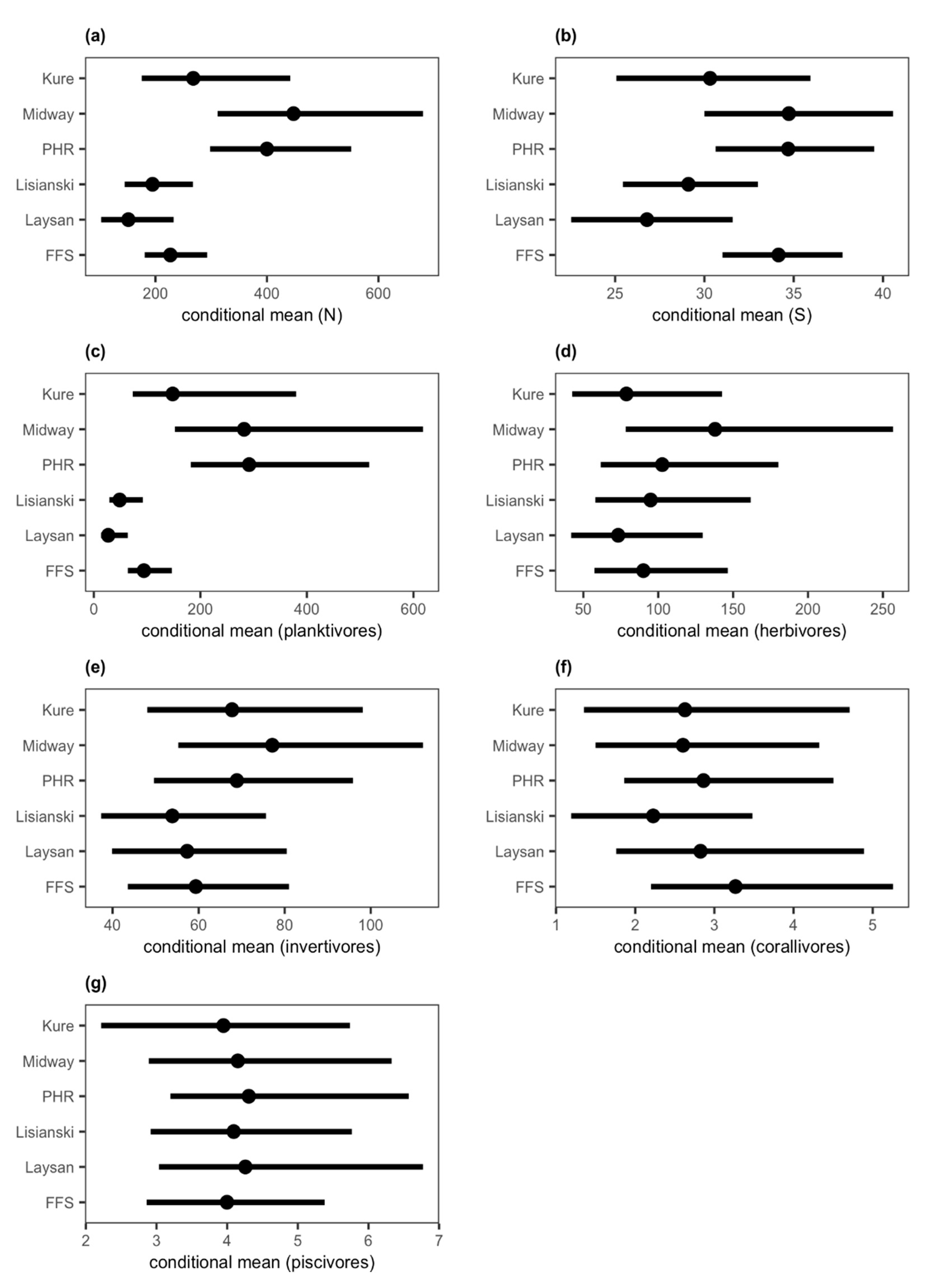
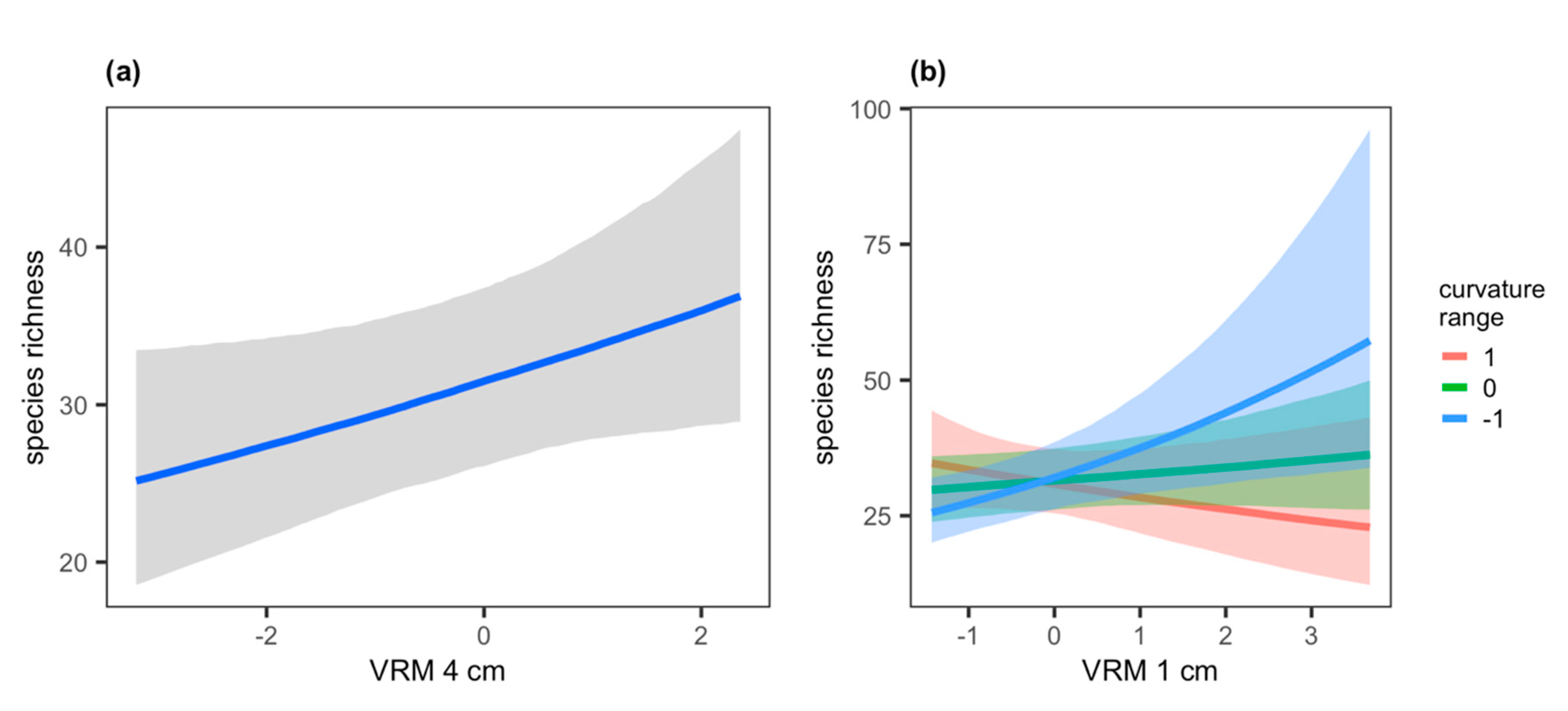
There were no apparent associations detected between the total fish abundance and either the habitat metrics or benthic cover variables. The final model only included the grouping factor (Table A1) explaining 26.9% of the variation in the total fish abundance and captured differences in the total fish abundance among the islands/atolls of the NWHI (Figure A1a). On the other hand, species richness was positively correlated with the mean VRM deviation at 4-cm resolution (Figure 2a, Table A1). Interactive effects of the mean VRM at 1-cm resolution and the curvature range were also detected (Table A1), with the association between species richness and the mean VRM at 1-cm resolution changing from positive to negative as the curvature range increased (Figure 2b). The grouping factor (geographical locations) alone explained 16.2% of the variation in species richness (Figure A1b), and the habitat variables explained an additional 11.7% for a total of 27.9% of the variation explained by the final model. The final model for species richness did not include any of the benthic cover variables (Table A1).
Similar to the total fish abundance, no apparent associations were detected for the abundances of planktivores and invertivores with either the habitat metrics or benthic cover variables (Table A1). The final model for the abundance of planktivores only included the grouping factor (Table A1) and explained 32.2% of the variation in the variable (Figure A1c). The final model for the abundance of invertivores included the grouping factor and depth, showing a potential decrease (95% CI = −0.04–0.00, Table A1) in invertivore abundance with depth, and explained 15.6% of the variation in the variable.
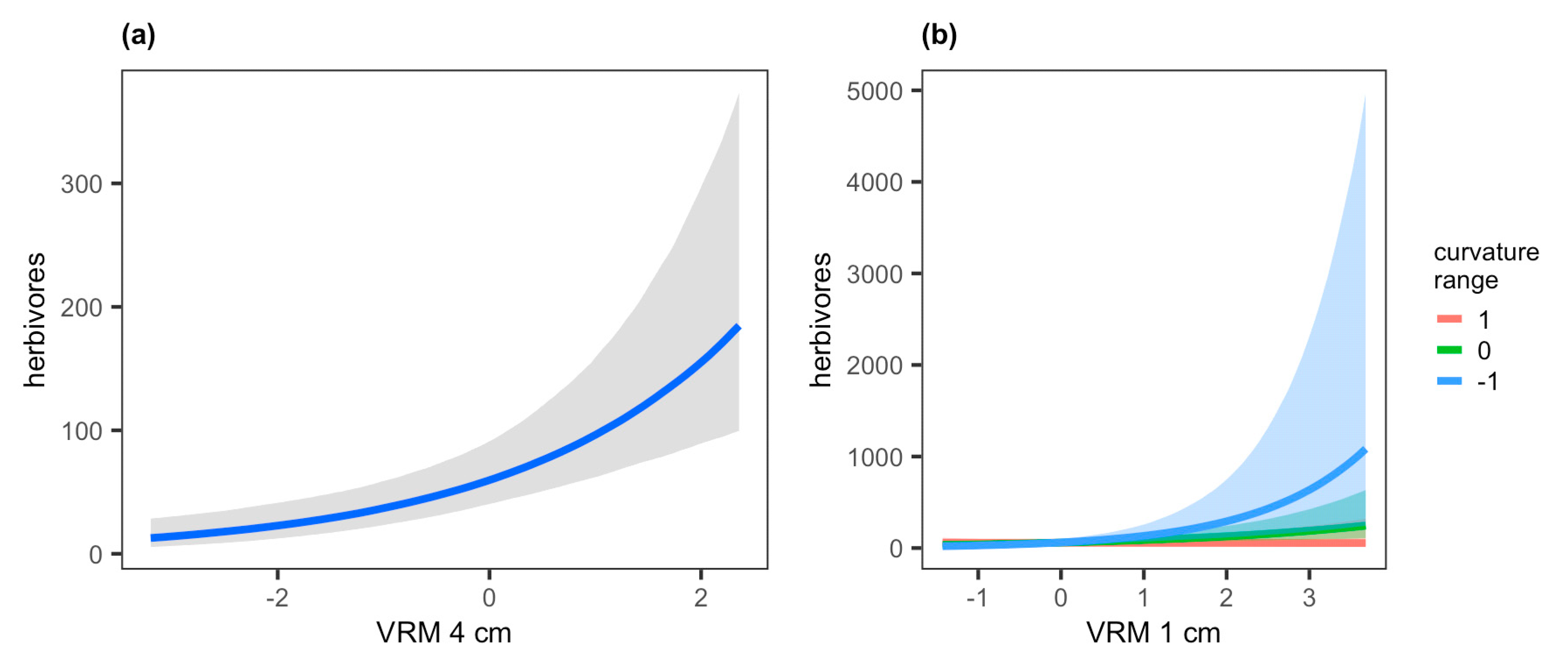
The abundance of herbivores was positively correlated with the mean VRM deviation at 4-cm resolution (Figure 3a, Table A1). Main effects of the mean VRM at 1-cm resolution and interactive effects of the mean VRM at 1-cm resolution and the curvature range were also detected (Table A1), with the abundance of herbivores increasing with an increase in the mean VRM at 1-cm resolution and this increase becoming larger as the curvature range decreased (Figure 3b). The grouping factor and depth, which showed a decrease in herbivore abundance with depth (Table A1), together explained 18.1% of the variation in the abundance of herbivore. The habitat variables explained an additional 28.2% for a total of 46.3% of the variation explained by the final model.
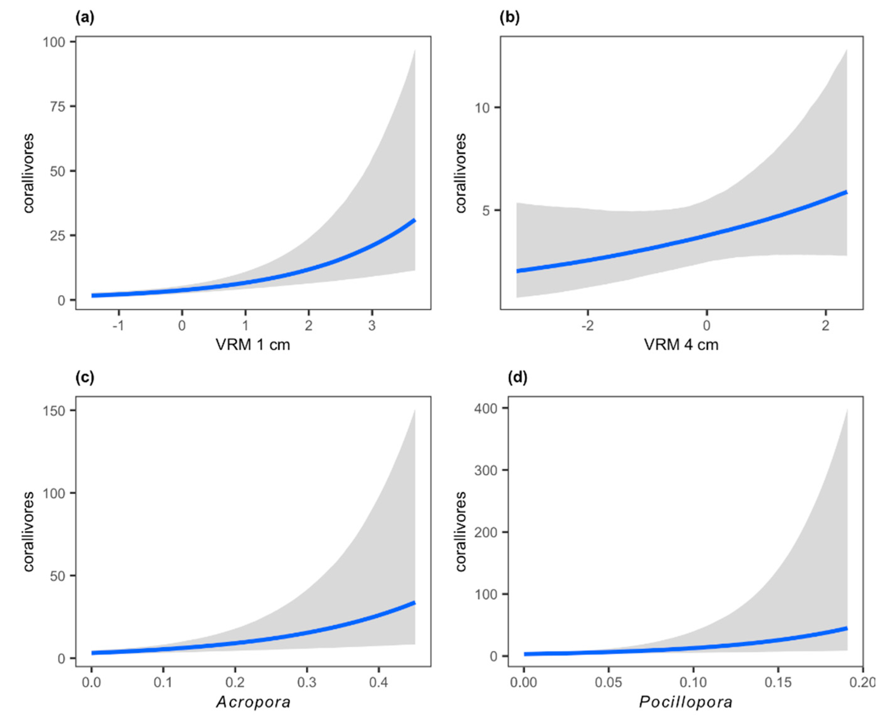
The abundance of corallivores was positively correlated with the mean VRM at 1-cm resolution, Acropora coral cover and Pocillopora coral cover (Figure 4, Table A1). There was also weak evidence for a positive association between the abundance of corallivores and the mean VRM deviation at 4-cm resolution (95% CI = −0.09–0.47, Table A1). The grouping factor alone explained 16.4% of the variation in the abundance of corallivores (Figure A1f), and the habitat variables explained an additional 32.0% for a total of 48.4% of the variation explained by the model. The two benthic cover variables, Acropora and Pocillopora coral covers, further explained an additional 11.6% for a total of 60.0% of the variation explained by the final model.
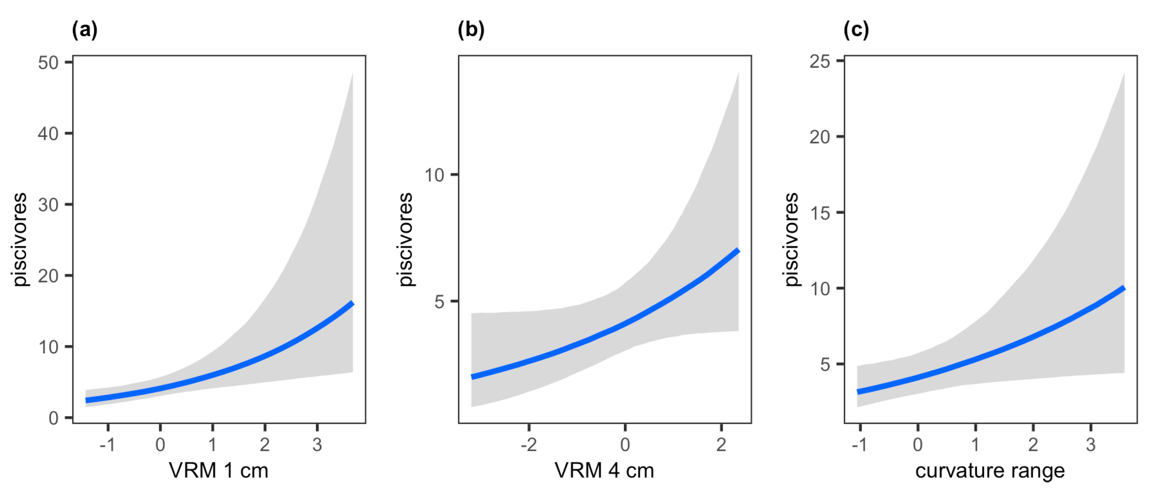
The abundance of piscivores was positively correlated with the mean VRM at 1-cm resolution and the curvature range (Figure 5, Table A1). Similar to the abundance of corallivores, there was also weak evidence for a positive association between the abundance of piscivores and the mean VRM deviation at 4-cm resolution (95% CI = −0.01–0.48, Table A1). The grouping factor alone explained only 1.9% of the variation in the abundance of piscivores, suggesting relatively low variability in the abundance of this trophic group among different islands/atolls of the NWHI. This was also confirmed in the plot of conditional means for different islands/atolls (Figure A1g). The three habitat variables explained an additional 22.8% of the variation in the abundance of piscivores, for a total of 24.7% of the variation explained by the final model.
Geographical locations (i.e., islands/atolls of the NWHI) and depth explained significant proportions of the variation in the structure of fish assemblages as a whole on the basis of Bray-Curtis dissimilarity (Table 1). Three habitat metrics (mean VRM at 1-cm resolution, mean VRM deviation at 4-cm resolution and curvature range) also explained statistically significant proportions of variation, each explaining an additional 2.1%, 6.0% and 1.8%, respectively (Table 1). None of the habitat interaction terms improved the model on the basis of AICc. Similarly, none of the benthic cover variables further improved the model on the basis of AICc after the habitat metrics were fitted. The final model including the five explanatory variables explained, in total, 43.2% of the variation in the structure of fish assemblages (Table 1).
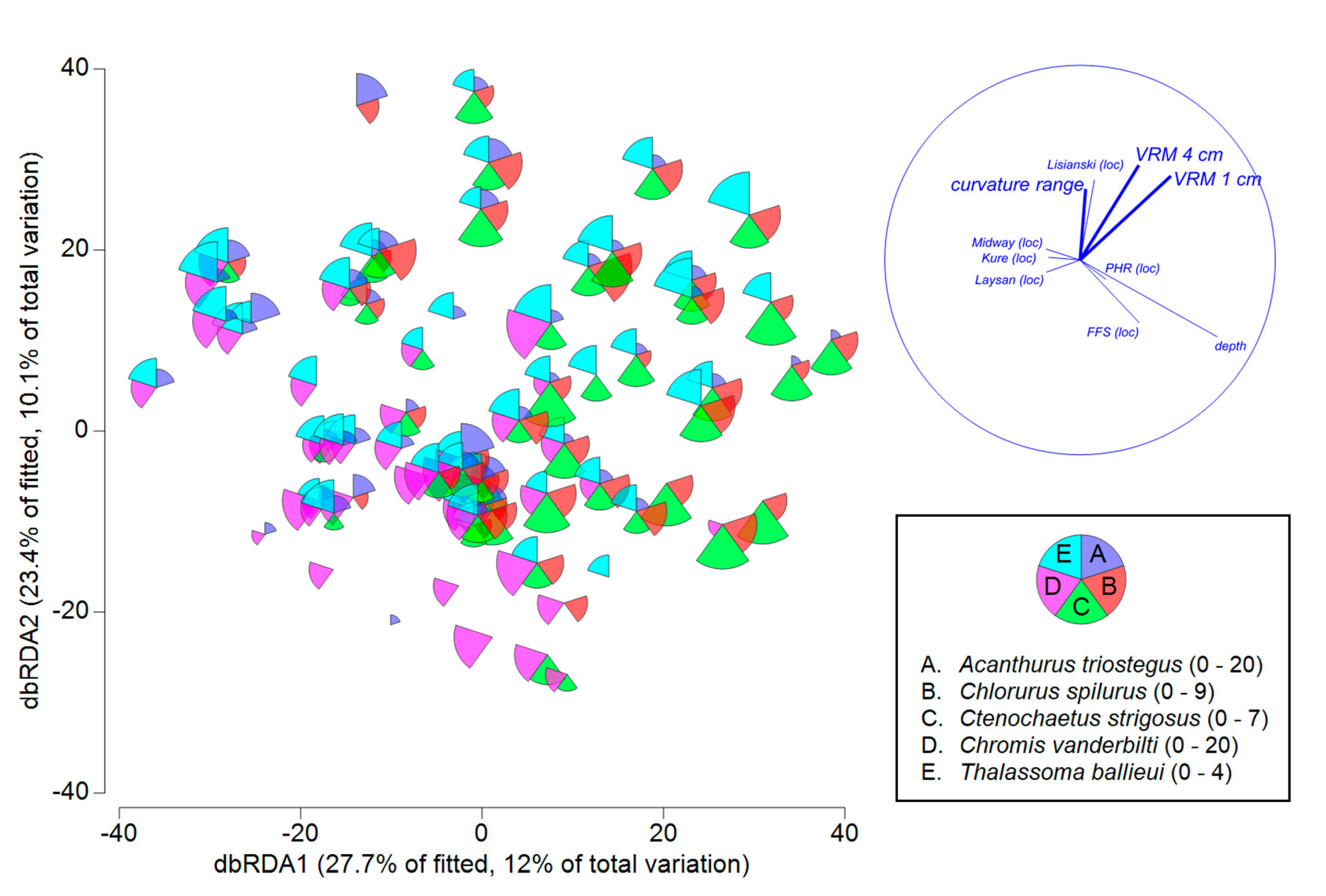
The exploratory analysis utilizing the CAP ordination with vector overlay identified five species of fish that were potentially associated with the habitat metrics based on multiple partial correlations of individual fish taxa with canonical axes (Figure S1). These included Acanthurus triostegus, Chlorurus spilurus, Chromis vanderbilti, Ctenochaetus strigosus and Thalassoma ballieui. Specifically, the abundances of C. spilurus and C. strigosus positively correlated with the mean VRM at 1-cm resolution and mean VRM deviation at 4-cm resolution, while the abundance of C. vanderbilti negatively correlated with these metrics. The abundance of A. triostegus positively correlated with the curvature range and mean VRM deviation at 4-cm resolution, and the abundance of T. ballieui positively correlated with the curvature range. For the purpose of data visualization, their abundances were superimposed on an ordination of the fitted values from the DISTLM model in Table 1 that was generated using distance-based redundancy analysis (Figure 6).

4. Discussion

The associations between fish assemblages and habitat metrics found in the present study were mostly positive, supporting previous findings that increases in the architectural complexity of habitats were linked to higher levels of fish abundance and diversity [1,2,3]. This overall relationship is likely due to increases in the architectural complexity, and thus in 3D space, resulting in increased amounts of resources for fish (e.g., food/prey and shelter) [1]. The use of photogrammetric techniques and resulting DEMs allowed us to comprehensively characterize the architectural complexity of coral reef habitats using three habitat metrics, with each metric quantifying architectural complexity provided by specific benthic features. Species richness was positively correlated with the mean VRM at 1-cm resolution, which captures the smaller-scale structural complexity of branching or encrusting corals (e.g., branching Pocillopora, branching Porites, encrusting Porites and encrusting Montipora) [16,28], when the curvature range was relatively low (Figure 2b). Species richness was also positively correlated with the mean VRM deviation at 4-cm resolution (Figure 2a), which additionally captures the larger-scale structural complexity of mounding and tabulate corals (e.g., mounding Porites and tabulate Acropora) [16,28]. The interactive effects of the mean VRM at 1-cm resolution and the curvature range were somewhat complex (Figure 2b). When the curvature range was high, which typically occurs when ledge-like structures or holes cause dramatic changes in elevation within a DEM [28], the number of fish species was higher for habitats with lower mean VRM values at 1-cm resolution than for those with higher values. This relationship may be due to sites with high levels of Acropora table coral cover supporting higher numbers of fish species because the curvature range captures the presence of “drops” from the table-top structures of the tabulate Acropora to surrounding surfaces [45]. Tabulate Acropora also creates large flat table-top areas resulting in a relatively low value of mean VRM at 1-cm resolution [45]. The distinct habitat architecture created by the dominance of Acropora corals with tabulate morphologies likely explains this unique interactive effect of high curvature values and low mean VRM values being associated with high species richness.
For different trophic groups, the mean VRM at 1-cm resolution was positively correlated with the abundances of herbivores, corallivores and piscivores, and the mean VRM deviation at 4-cm resolution was positively correlated with the abundance of herbivores. The effects of curvature range were dependent on the trophic groups: the curvature range was positively correlated with the abundance of piscivores but mostly negatively correlated with the abundance of herbivores, although the effect of the curvature range on the abundances of herbivores was also affected by the mean VRM at 1-cm resolution. Differences in herbivore abundance predicted from the curvature range were relatively small when the mean VRM at 1-cm resolution was low (Figure 3b). These differences among trophic groups provide us with some insights regarding how different trophic groups utilize their habitats. Piscivores seem to prefer an architecturally complex habitat in terms of both benthic cover and surface topography potentially due to increased availability of refuges and prey [46,47], while small-bodied corallivores (mostly butterflyfish and damselfish in the present study, see below for more details) seem to prefer habitats with high levels of small-scale architectural complexity associated with branching and/or encrusting corals. Herbivores (mostly surgeonfish and parrotfish in the present study) generally have larger body sizes than corallivores in the NWHI [31] and seem to prefer habitats with high levels of both small- and large-scale architectural complexity associated with all types of coral morphologies, but not necessarily habitats with high architectural complexity associated with surface topography (e.g., ledge-like structure or holes). These findings demonstrate the advantage of utilizing photogrammetric techniques and DEMs to characterize benthic habitats, as different habitat metrics obtained from DEMs can separate the architectural complexity arising from benthos and surface topographies, which would be difficult when using conventional in situ measurements like the chain-and-tape rugosity [12].
Unlike the other trophic groups in the present study, corallivores were associated with benthic cover (Acropora and Pocillopora corals) even after the effects of habitat metrics were considered. Corallivores found in the present study were primarily Plectroglyphidodon johnstonianus, Chaetodon multicinctus and Chaetodon trifascialis, with these three species accounting for nearly 85% of all corallivores. P. johnstonianus is closely associated with both Acropora and Pocillopora corals and feeds primarily on coral polyps [31,48]. C. multicinctus feeds mainly on coral polyps including Porites lobata, Porites compressa and Pocillopora meandrina [31] but prefers P. meandrina potentially due to its higher energy content than the two Porites species [49,50]. C. trifascialis also feeds primarily on Acropora, and, in Hawai‘i, it occurs commonly only at French Frigate Shoals where Acropora is abundant [51,52]. This species has been suggested as a potential indicator species to detect changes in the distribution of Acropora table corals due to their co-evolutionary association [51], although a single C. trifascialis has been reported from the island of O’ahu swimming within branches of a P. meandrina colony [53]. The inclusion of Acropora and Pocillopora coral covers in the final model likely reflects the strong associations of the three dominant corallivores with these corals, highlighting the importance of the distribution of food source, in addition to habitat structure, for corallivores in the NWHI.
For the individual species identified to be potentially associated with habitat metrics, Chlorurus spilurus, Ctenochaetus strigosus and Acanthurus triostegus are herbivores, although C. strigosus also feeds on detritus [31,54]. The positive associations of C. spilurus and C. strigosus with the two VRM metrics were consistent with the general pattern of herbivores. Both C. strigosus and C. spilurus (the latter formerly misidentified as Scarus sordidus in Hawai’i) are more abundant in coral-rich habitats than other types of habitats in Hawai’i [39], and C. spilurus has been reported to have the strongest association with live coral among Hawaiian scarids [55]. Scarid juveniles including C. spilurus use branching corals, particularly Porites compressa, as nursery habitats [56], while C. strigosus favors relatively deep P. compressa-rich habitats as juveniles, followed by an ontogenetic shift to shallower turf-rich habitats as adults [57]. The distributions of herbivores in general and specifically of C. spilurus and C. strigosus highlight the importance of the architectural complexity of habitats for herbivores. The distribution of macroalgae (i.e., their potential food resource) does not seem to be a major factor for their distributions in the NWHI, which contrasts with the pattern observed with corallivores. While most corallivores in the present study have strict preference for their diet as previously mentioned, herbivores in the NWHI do not necessary feed on macroalgae (e.g., grazers) [31], which may explain the observed difference between corallivores and herbivores.
The herbivorous A. triostegus exhibited a somewhat different pattern from the one observed with C. strigosus and C. spilurus. A. triostegus is the most abundant surgeonfish in Hawai’i and occurs in a variety of habitats, but it is generally not highly abundant in areas of high live coral cover [58]. A. triostegus mostly feeds on relatively fine filamentous algae [58] and is often observed grazing on turf algae growing on relatively open hard substrata (authors’ personal observations). Sale [59] observed that juvenile A. triostegus often stayed close to cover during feeding. The positive associations of this species, including both juveniles and adults, with the mean VRM deviation at 4-cm resolution and the curvature range found in the present study (Supplementary Figure S1a) may be related to this feeding behavior where A. triostegus grazes on filamentous algae growing on a relatively flat surface while staying adjacent to some types of cover provided by the architectural complexity associated with mounding corals and/or surface topography. Barlow [60] speculated that schooling by A. triostegus may serve dual purposes under different circumstances: in areas of high coral cover, it assists in swamping territorial herbivores (e.g., Acanthurus nigrofuscus), whereas in reef-flat areas of a low-shelter atoll, it may serve an anti-predator function. The latter use of schooling behavior may enable A. triostegus to forage in habitats with a lower availability of shelter than those used by solitary herbivores, resulting in the positive association of this species with the architectural complexity at a larger spatial scale than other herbivores.
The total fish abundance and the abundances of planktivores and invertivores did not show associations with either habitat metrics or benthic cover. The final models for the total abundance and planktivore abundance were relatively similar likely due to the overall high abundance of planktivores in the present study also driving the pattern observed with the total fish abundance. Thresher [61] found that abundance of planktivores was more strongly correlated with current strength and predator abundance rather than topographic complexity or cover by branching corals, although the distributions of diurnally active planktivores were species specific. In the present study, despite the lack of overall association with habitat metrics for planktivores and invertivores, Chromis vanderbilti (planktivore) and Thalassoma ballieui (invertivore) were identified in the CAP analysis to be negatively associated with the two VRM metrics and positively associated with the curvature range, respectively (Figure 6). This highlights the limitation of generalizing the habitat-fish interactions at the level of functional guilds (e.g., planktivore, herbivore, etc.) and the importance of formal assessments with individual species when there are specific species of interest a priori or data analyses reveal potential species of importance. Here, the pattern observed with C. vanderbilti was perplexing, as this small-bodied planktivore uses reefs as shelters and stays close to the bottom even while feeding [31]; 3D structure of corals should provide them with shelter space, so we would have expected positive, not negative, associations between this species and the two VRM metrics. C. vanderbilti is highly abundant on forereefs of the NWHI at depths of <18 m [32]. In Moorea, French Polynesia, C. vanderbilti is found exclusively on the outer reef [62]. The relatively high levels of wave energy experienced on outer reefs likely limit the architectural complexity of corals, and this might have affected the overall pattern of C. vanderbilti distribution captured in the CAP analysis.
The present study focused on examining the effects of habitat metrics on the distribution and abundance of reef fish in the NWHI and evaluated whether benthic cover could explain any additional variation in the fish data after the habitat metrics were considered. The study was motivated by the current bottleneck with image annotation that coral reef monitoring programs often encounter and by the availability of cutting-edge photogrammetric techniques that allow for detailed quantitative characterization of habitat structure. The study was, therefore, not designed to evaluate the relative importance of habitat metrics versus benthic cover. Habitat metrics are strongly influenced by benthic cover. In the NWHI, for example, tabulate Acropora generates relatively low VRM values at 1-cm resolution and highly variable curvature values [16,45], while branching Pocillopora and Porites (e.g., Porites compressa) generate relatively high VRM values at 1-cm resolution [16,28]. Encrusting and mounding Porites (e.g., Porites lobata) and encrusting Montipora generate high VRM values at lower resolutions than branching corals, with a mounding growth form being captured well at 4-cm resolution [16,28]. In our previous study, up to ≈70% of variation in these habitat metrics were explained by benthic cover [16]. Previous studies investigating the effects of both habitats’ physical structure and benthic community composition have found both types of data to be important for the structure of fish assemblages [63] or benthic community composition to be more important than habitat structure [2]. Richardson et al. [64] also reported shifts in fish assemblages shortly after a mass coral bleaching event while the carbonate structures of hard corals were still mostly intact. These studies underscore the importance of collecting data on benthic community composition in coral-reef monitoring, and particularly, such data are essential when assessing the status and health of coral assemblages.
The present study clearly demonstrated that a combination of habitat metrics that were specifically chosen to capture the architectural complexity of coral reefs provided by both benthic organisms and surface topography could be used in a monitoring study to account for the effects of habitats on the fish assemblages of the NWHI. While the amount of variation explained by the habitat metrics varied depending on the response variables (e.g., fish species richness and abundances by trophic categories), benthic cover did not explain additional variation with the exception of the abundance of corallivores. As the frequency and severity of environmental stress are predicted to increase [65], the need for well-designed coral-reef monitoring programs also increase. Scientists and managers may need to prioritize processing of their monitoring data in order to keep up with a frequent inflex of data and make timely decisions for management. The results of the present study provide us with important information to strategize resource allocations for different components of coral-reef monitoring and to detect any changes in fish assemblages while appropriately accounting for their changing habitats.

Supplementary Materials

The following are available online at https://www.mdpi.com/1424-2818/12/11/430/s1, Figure S1: Canonical analysis of principal coordinates (CAP) constrained ordinations for the fish data from the 80 survey sites on the basis of Bray-Curtis dissimilarity calculated on square-root transformed abundance.

Author Contributions

Conceptualization, A.F. and J.H.R.B.; methodology, A.F.; validation, A.F., R.K.K., K.H.P., and J.H.R.B.; formal analysis, A.F.; writing—original draft preparation, A.F.; writing—review and editing, A.F., R.K.K., K.H.P., and J.H.R.B.; visualization, A.F.; funding acquisition, R.K.K. and J.H.R.B. All authors have read and agreed to the published version of the manuscript.

Funding

This work was funded by the National Oceanic and Atmospheric Administration’s Office of National Marine Sanctuaries through the Papahānaumokuākea Marine National Monument, by the National Science Foundation under the CREST-PRF Award #1720706 and EPSCoR Program Award OIA #1557349 to J.H.R. Burns, and by the National Fish and Wildlife Foundation under Award # NFWF-UHH-059023 to J.H.R. Burns.

Acknowledgments

We thank the officers and crew of NOAA ship Hi’ialakai for logistic support and field assistance, and Jason Leonard, Jake Asher, Roseanna Lee and Colton Johnson for the fish surveys and the collection of benthic imagery. We also thank Sofia Ferreira Colman, Jazmin Helzer, Brittany Wells, Shane Murphy, Mia Lamirand and Brianna Craig for the annotations of orthophotomosaics, and three anonymous reviewers who improved the manuscript through their input. The scientific results and conclusions, as well as any views or opinions expressed herein, are those of the authors and do not necessarily reflect the views of the National Oceanic and Atmospheric Administration (NOAA) or the U.S. Department of Commerce.

Conflicts of Interest

The authors declare no conflict of interest.

Appendix A

Figure A1. Conditional means of fish abundance at different geographic locations, French Frigate Shoals (FFS), Laysan Island (Laysan), Lisianski Island (Lisianski), Pearl and Hermes Atoll (PHR), Midway Atoll (Midway) and Kure Atoll (Kure), based on the respective final models for (a) the total fish abundance, (b) species richness and the abundances of (c) planktivores, (d) herbivores, (e) invertivores, (f) corallivores and (g) piscivores.
Diversity 12 00430 g0a1
Table A1. Parameter estimates for the generalized linear models with the negative binomial probability distribution with the log link function. Estimates of coefficients for the fixed terms (depth, standardized mean VRM at 1-cm resolution, standardized mean VRM deviation at 4-cm resolution, standardized curvature range, interaction between the standardized mean VRM at 1-cm resolution and the standardized curvature range and percent covers of Acropora and Pocillopora corals) are shown along with their 95% CI in the parentheses. The estimates whose 95% CI did not overlap with 0 are shown in bold and marked with asterisks (*). Fixed terms that were not included in the final model for any of the response variables are not included in this table. Estimates of standard deviation for the grouping factor, geographical locations, are also shown (sd(loc)) along with their 95% CI in the parentheses. Conditional means of each response variable for different geographical locations are also shown in Figure A1.
DepthVRM 1 cmVRM Deviation
4 cm
Curvature RangeVRM 1 cm × Curvature RangeAcroporaPocilloporasd (loc)
total abundance-------0.63
(0.25–1.50)
species richness-0.04
(−0.04–0.11)
0.07 *
(0.00–0.14)
−0.02
(−0.09–0.06)
−0.12 *
(−0.24–0.00)
--0.18
(0.05–0.45)
planktivores-------1.39
(0.59–3.33)
herbivores−0.03 *
(−0.06–−0.01)
0.39 *
(0.18–0.60)
0.48 *
(0.27–0.71)
−0.03
−0.23–0.18
−0.39 *
(−0.72–−0.06)
--0.38
(0.04–1.05)
invertivores−0.02 *
(−0.04–0.00)
------0.23
(0.03–0.61)
corallivores-0.58 *
(0.31–0.87)
0.19
(−0.09–0.47)
--5.33 *
(2.17–8.69)
14.18 *
(4.81–25.78)
0.32
(0.02–0.93)
piscivores-0.38 *
(0.13–0.65)
0.23
(−0.01–0.48)
0.25 *
(0.02–0.48)
---0.19
(0.01–0.67)

References

  1. Graham, N.A.J.; Nash, K.L. The importance of structural complexity in coral reef ecosystems. Coral Reefs 2013, 32, 315–326. [Google Scholar] [CrossRef]
  2. Komyakova, V.; Munday, P.L.; Jones, G.P. Relative importance of coral cover, habitat complexity and diversity in determining the structure of reef fish communities. PLoS ONE 2013, 8, e83178. [Google Scholar] [CrossRef] [PubMed]
  3. Holbrook, S.J.; Brooks, A.J.; Schmitt, R.J. Variation in structural attributes of patch-forming corals and in patterns of abundance of associated fishes. Mar. Freshw. Res. 2002, 53, 1045–1053. [Google Scholar] [CrossRef]
  4. Floeter, S.R.; Krohling, W.; Gasparini, J.L.; Ferreira, C.E.L.; Zalmon, I.R. Reef fish community structure on coastal islands of the southeastern Brazil: The influence of exposure and benthic cover. Environ. Biol. Fish. 2007, 78, 147–160. [Google Scholar] [CrossRef]
  5. Hourigan, T.F. Environmental determinants of butterflyfish social systems. Environ. Biol. Fish. 1989, 25, 61–78. [Google Scholar] [CrossRef]
  6. Burns, J.H.R.; Delparte, D.; Gates, R.D.; Takabayashi, M. Integrating structure-from-motion photogrammetry with geospatial software as a novel technique for quantifying 3D ecological characteristics of coral reefs. PeerJ 2015, 3, e1077. [Google Scholar] [CrossRef]
  7. Burns, J.H.R.; Delparte, D.; Kapono, L.; Belt, M.; Gates, R.D.; Takabayashi, M. Assessing the impact of acute disturbances on the structure and composition of a coral community using innovative 3D reconstruction techniques. Methods Oceanogr. 2016, 15–16, 49–59. [Google Scholar] [CrossRef] [Green Version]
  8. Figueira, W.; Ferrari, R.; Weatherby, E.; Porter, A.; Hawes, S.; Byrne, M. Accuracy and precision of habitat structural complexity metrics derived from underwater photogrammetry. Remote Sens. 2015, 7, 16883–16900. [Google Scholar] [CrossRef] [Green Version]
  9. Bryson, M.; Ferrari, R.; Figueira, W.; Pizarro, O.; Madin, J.; Williams, S.; Byrne, M. Characterization of measurement errors using structure-from-motion and photogrammetry to measure marine habitat structural complexity. Ecol. Evol. 2017, 7, 5669–5681. [Google Scholar] [CrossRef]
  10. Raoult, V.; Reid-Anderson, S.; Ferri, A.; Williamson, J.E. How reliable is structure from motion (SfM) over time and between observers? A case study using coral reef bommies. Remote Sens. 2017, 9, 740. [Google Scholar]
  11. Fukunaga, A.; Burns, J.H.R.; Craig, B.K.; Kosaki, R.K. Integrating three-dimensional benthic habitat characterization techniques into ecological monitoring of coral reefs. J. Mar. Sci. Eng. 2019, 7, 27. [Google Scholar] [CrossRef] [Green Version]
  12. Risk, M.J. Fish diversity on a coral reef in the Virgin Islands. Atoll Res. Bull. 1972, 153, 1–4. [Google Scholar] [CrossRef] [Green Version]
  13. Walbridge, S.; Slocum, N.; Pobuda, M.; Wright, D.J. Unified geomorphological analysis workflows with Benthic Terrain Modeler. Geosciences 2018, 8, 94. [Google Scholar] [CrossRef] [Green Version]
  14. Young, G.C.; Dey, S.; Rogers, A.D.; Exton, D. Cost and time-effective method for multi-scale measures of rugosity, fractal dimension, and vector dispersion from coral reef 3D models. PLoS ONE 2017, 12, e0175341. [Google Scholar] [CrossRef] [PubMed]
  15. Burns, J.H.R.; Fukunaga, A.; Pascoe, K.H.; Runyan, A.; Craig, B.K.; Talbot, J.; Pugh, A.; Kosaki, R.K. 3D habitat complexity of coral reefs in the Northwestern Hawaiian Islands is driven by coral assemblage structure. In Underwater 3D Recording & Modelling: A Tool for Modern Applications and CH Recording; The International Archives of the Photogrammetry, Remote Sensing and Spatial Information Sciences: Limassol, Cyprus, 2019; Volume XLII-2/W10, pp. 61–67. [Google Scholar]
  16. Fukunaga, A.; Burns, J.H.R.; Pascoe, K.H.; Kosaki, R.K. Associations between benthic cover and habitat complexity metrics obtained from 3D reconstruction of coral reefs at different resolutions. Remote Sens. 2020, 12, 1011. [Google Scholar] [CrossRef] [Green Version]
  17. Williams, I.D.; Couch, C.S.; Beijbom, O.; Oliver, T.A.; Vargas-Angel, B.; Schumacher, B.D.; Brainard, R.E. Leveraging automated image analysis tools to transform our capacity to assess status and trends of coral reefs. Front. Mar. Sci. 2019, 6, 222. [Google Scholar] [CrossRef] [Green Version]
  18. González-Rivero, M.; Beijbom, O.; Rodriguez-Ramirez, A.; Bryant, D.E.P.; Ganase, A.; Gonzalez-Marrero, Y.; Herrera-Reveles, A.; Kennedy, E.V.; Kim, C.J.S.; Lopez-Marcano, S.; et al. Monitoring of coral reefs using artificial intelligence: A feasible and cost-effective approach. Remote Sens. 2020, 12, 489. [Google Scholar] [CrossRef] [Green Version]
  19. Hopkinson, B.M.; King, A.C.; Owen, D.P.; Johnson-Roberson, M.; Long, M.H.; Bhandarkar, S.M. Automated classification of three-dimensional reconstructions of coral reefs using convolutional neural networks. PLoS ONE 2020, 15, e0230671. [Google Scholar] [CrossRef]
  20. Williams, I.D.; Baum, J.K.; Heenan, A.; Hanson, K.M.; Nadon, M.O.; Brainard, R.E. Human, oceanographic and habitat drivers of central and western Pacific coral reef fish assemblages. PLoS ONE 2015, 10, e0120516. [Google Scholar] [CrossRef]
  21. Bohnsack, J.A.; Bannerot, S.P. A Stationary Visual Census Technique for Quantitatively Assessing Community Structure of Coral Reef Fishes; NOAA Technical Report NMFS 41; U.S. Department of Commerce, National Oceanic and Atmospheric Administration, National Marine Fisheries Service: Silver Spring, MD, USA, 1986; p. 15. [Google Scholar]
  22. R Core Team. R: A Language and Environment for Statistical Computing, 3.6.2; R Foundation for Statistical Computing: Vienna, Austria, 2019. [Google Scholar]
  23. Beijbom, O.; Edmunds, P.J.; Roelfsema, C.; Smith, J.; Kline, D.I.; Neal, B.P.; Dunlap, M.J.; Moriarty, V.; Fan, T.-Y.; Tan, C.-J.; et al. Towards automated annotation of benthic survey images: Variability of human experts and operational modes of automation. PLoS ONE 2015, 10, e0130312. [Google Scholar] [CrossRef]
  24. Pebesma, E.J.; Bivand, R.S. Classes and methods for spatial data in R. R News 2005, 5, 9–13. [Google Scholar]
  25. Bivand, R.S.; Pebesma, E.; Gómez-Rubio, V. Applied Spatial Data Analysis with R, 2nd ed.; Springer: New York, NY, USA, 2013. [Google Scholar]
  26. Hijmans, R.J. Raster: Geographic Data Analysis and Modeling. R Package Version 3.0-7. 2019. Available online: https://CRAN.R-project.org/package=raster (accessed on 12 May 2020).
  27. Bivand, R.; Rundel, C. Rgeos: Interface to Geometry Engine—Open Source (GEOS). R Package Version 0.5-2. 2019. Available online: https://CRAN.R-project.org/package=rgeos (accessed on 12 May 2020).
  28. Fukunaga, A.; Burns, J.H.R. Metrics of coral reef structural complexity extracted from 3D mesh models and Digital Elevation Models. Remote Sens. 2020, 12, 2676. [Google Scholar] [CrossRef]
  29. Sappington, J.M.; Longshore, K.M.; Thompson, D.B. Quantifying landscape ruggedness for animal habitat analysis: A case study using bighorn sheep in the Mojave Desert. J. Wildl. Manage. 2007, 71, 1419–1426. [Google Scholar] [CrossRef]
  30. Zevenbergen, L.W.; Thorne, C.R. Quantitative analysis of land surface topography. Earth Surf. Process. Landf. 1987, 12, 47–56. [Google Scholar] [CrossRef]
  31. Randall, J.E. Reef and Shore Fishes of the Hawaiian Islands; Sea Grant College Program, University of Hawaii: Honolulu, HI, USA, 2007; p. 546. [Google Scholar]
  32. Fukunaga, A.; Kosaki, R.K. Use of multivariate control charts to assess the status of reef fish assemblages in the Northwestern Hawaiian Islands. PeerJ 2017, 5, e3651. [Google Scholar] [CrossRef] [PubMed] [Green Version]
  33. Bürkner, P.-C. brms: An R package for Bayesian multilevel models using Stan. J. Stat. Softw. 2017, 80, 1–28. [Google Scholar] [CrossRef] [Green Version]
  34. Bürkner, P.-C. Advanced Bayesian multilevel modeling with the R package brms. R J. 2018, 10, 395–411. [Google Scholar] [CrossRef]
  35. Eddelbuettel, D.; François, R. Rcpp: Seamless R and C++ integration. J. Stat. Softw. 2011, 40, 1–18. [Google Scholar] [CrossRef] [Green Version]
  36. Eddelbuettel, D. Seamless R and C++ Integration with Rcpp; Springer: New York, NY, USA, 2013; p. 220. [Google Scholar]
  37. Eddelbuettel, D.; Balamuta, J.J. Extending R with C++: A brief introduction to Rcpp. PeerJ Preprints 2017, 5, e3188v3181. [Google Scholar] [CrossRef]
  38. Hiatt, R.W.; Strasburg, D.W. Ecological relationships of the fish fauna on coral reefs of the Marshall Islands. Ecol. Monogr. 1960, 30, 65–127. [Google Scholar] [CrossRef]
  39. Hobson, E.S. Feeding relationships of teleostean fishes on coral reefs in Kona, Hawaii. Fish. Bull. 1974, 72, 915–1031. [Google Scholar]
  40. Hoover, J.P. Hawaii’s Fish; Mutual Publishing: Honolulu, HI, USA, 1993; p. 183. [Google Scholar]
  41. Legendre, P.; Anderson, M.J. Distance-based redundancy analysis: Testing multispecies responses in multifactorial ecological experiments. Ecol. Monogr. 1999, 69, 1–24. [Google Scholar] [CrossRef]
  42. McArdle, B.H.; Anderson, M.J. Fitting multivariate models to community data: A comment on distance-based redundancy analysis. Ecology 2001, 82, 290–297. [Google Scholar] [CrossRef]
  43. Anderson, M.J.; Robinson, J. Generalized discriminant analysis based on distances. Aust. N. Z. J. Stat. 2003, 45, 3301–3318. [Google Scholar] [CrossRef]
  44. Anderson, M.J.; Willis, T.J. Canonical analysis of principal coordinates: A useful method of constrained ordination for ecology. Ecology 2003, 84, 511–525. [Google Scholar] [CrossRef]
  45. Pascoe, K.H.; Fukunaga, A.; Kosaki, R.K.; Burns, J.H.R. 3D assessment of a coral reef in the Northwestern Hawaiian Islands reveals varying responses of habitat metrics following a catastrophic hurricane. (manuscript in preparation).
  46. Hixon, M.A.; Beets, J.P. Predation, prey refuges, and the structure of coral-reef fish assemblages. Ecol. Monogr. 1993, 63, 77–101. [Google Scholar] [CrossRef] [Green Version]
  47. Alvarez-Filip, L.; Gill, J.A.; Dulvy, N.K. Complex reef architecture supports more small-bodied fishes and longer food chains on Caribbean reefs. Ecosphere 2011, 2, 1–17. [Google Scholar] [CrossRef]
  48. Gochfeld, D.J. Energetics of a predator-prey interaction: Corals and coral-feeding fishes. Pac. Sci. 1991, 45, 246–256. [Google Scholar]
  49. Tricas, T.C. Prey selection by coral-feeding butterflyfishes: Strategies to maximize the profit. Environ. Biol. Fish. 1989, 25, 171–185. [Google Scholar] [CrossRef]
  50. Hourigan, T.F.; Tricas, T.C.; Reese, E.S. Coral reef fishes as indicators of environmental stress in coral reefs. In Marine Organisms as Indicators; Soule, D.F., Kleppel, G.S., Eds.; Springer: New York, NY, USA, 1988; pp. 107–135. [Google Scholar]
  51. Reese, E.S. Predation on corals by fishes of the family Chaetodontidae: Implications for conservation and management of coral reef ecosystems. Bull. Mar. Sci. 1981, 31, 594–604. [Google Scholar]
  52. Irons, D.K. Temporal and areal feeding behavior of the butterflyfish, Chaetodon trifascialis, at Johnston Atoll. Environ. Biol. Fish. 1989, 25, 187–193. [Google Scholar] [CrossRef]
  53. Franklin, E.C. Vagrancy in paradise: Documentation of the chevron butterflyfish Chaetodon trifascialis in Kaneohe Bay, Oahu, Hawaiian islands. Mar. Biodivers. Rec. 2017, 10, 22. [Google Scholar] [CrossRef] [Green Version]
  54. Jones, R.S. Ecological relationships in Hawaiian and Johnston Island Acanthuridae (Surgeonfishes). Micronesica 1968, 4, 309–361. [Google Scholar]
  55. Howard, K.G.; Schumacher, B.D.; Parrish, J.D. Community structure and habitat associations of parrotfishes on Oahu, Hawaii. Environ. Biol. Fish. 2009, 85, 175–186. [Google Scholar] [CrossRef]
  56. DeMartini, E.; Jokiel, P.; Beets, J.; Stender, Y.; Storlazzi, C.; Minton, D.; Conklin, E. Terrigenous sediment impact on coral recruitment and growth affects the use of coral habitat by recruit parrotfishes (F. Scaridae). J. Coast. Conserv. 2013, 17, 417–429. [Google Scholar] [CrossRef]
  57. Ortiz, D.M.; Tissot, B.N. Evaluating ontogenetic patterns of habitat use by reef fish in relation to the effectiveness of marine protected areas in West Hawaii. J. Exp. Mar. Biol. Ecol. 2012, 432–433, 83–93. [Google Scholar] [CrossRef]
  58. Randall, J.E. A contribution to the biology of the convict surgeonfish of the Hawaiian Islands, Acanthurus triostegus sandoicensis. Pac. Sci. 1961, 15, 215–272. [Google Scholar]
  59. Sale, P.F. Pertinent stimuli for habitat selection by the juvenile manini, Acanthurus triostegus sandvicensis. Ecology 1969, 50, 616–623. [Google Scholar] [CrossRef]
  60. Barlow, G.W. Extraspecific imposition of social grouping among surgeonfishes (Pisces: Acanthuridae). J. Zool. 1974, 174, 333–340. [Google Scholar] [CrossRef]
  61. Thresher, R.E. Environmental correlates of the distribution of planktivorous fishes in the One Tree reef lagoon. Mar. Ecol. Prog. Ser. 1983, 10, 137–145. [Google Scholar] [CrossRef]
  62. Gajdzik, L.; Parmentier, E.; Sturaro, N.; Frédérich, B. Trophic specializations of damselfishes are tightly associated with reef habitats and social behaviours. Mar. Biol. 2016, 163, 249. [Google Scholar] [CrossRef]
  63. Agudo-Adriani, E.A.; Cappelletto, J.; Cavada-Blanco, F.; Cróquer, A. Structural complexity and benthic cover explain reef-scale variability of fish assemblages in Los Roques National Park, Venezuela. Front. Mar. Sci. 2019, 6, 690. [Google Scholar] [CrossRef] [Green Version]
  64. Richardson, L.E.; Graham, N.A.J.; Pratchett, M.S.; Eurich, J.G.; Hoey, A.S. Mass coral bleaching causes biotic homogenization of reef fish assemblages. Glob. Change Biol. 2018, 24, 3117–3129. [Google Scholar] [CrossRef] [PubMed] [Green Version]
  65. Hughes, T.P.; Kerry, J.T.; Baird, A.H.; Connolly, S.R.; Dietzel, A.; Eakin, C.M.; Heron, S.F.; Hoey, A.S.; Hoogenboom, M.O.; Liu, G.; et al. Global warming transforms coral reef assemblages. Nature 2018, 556, 492–496. [Google Scholar] [CrossRef]
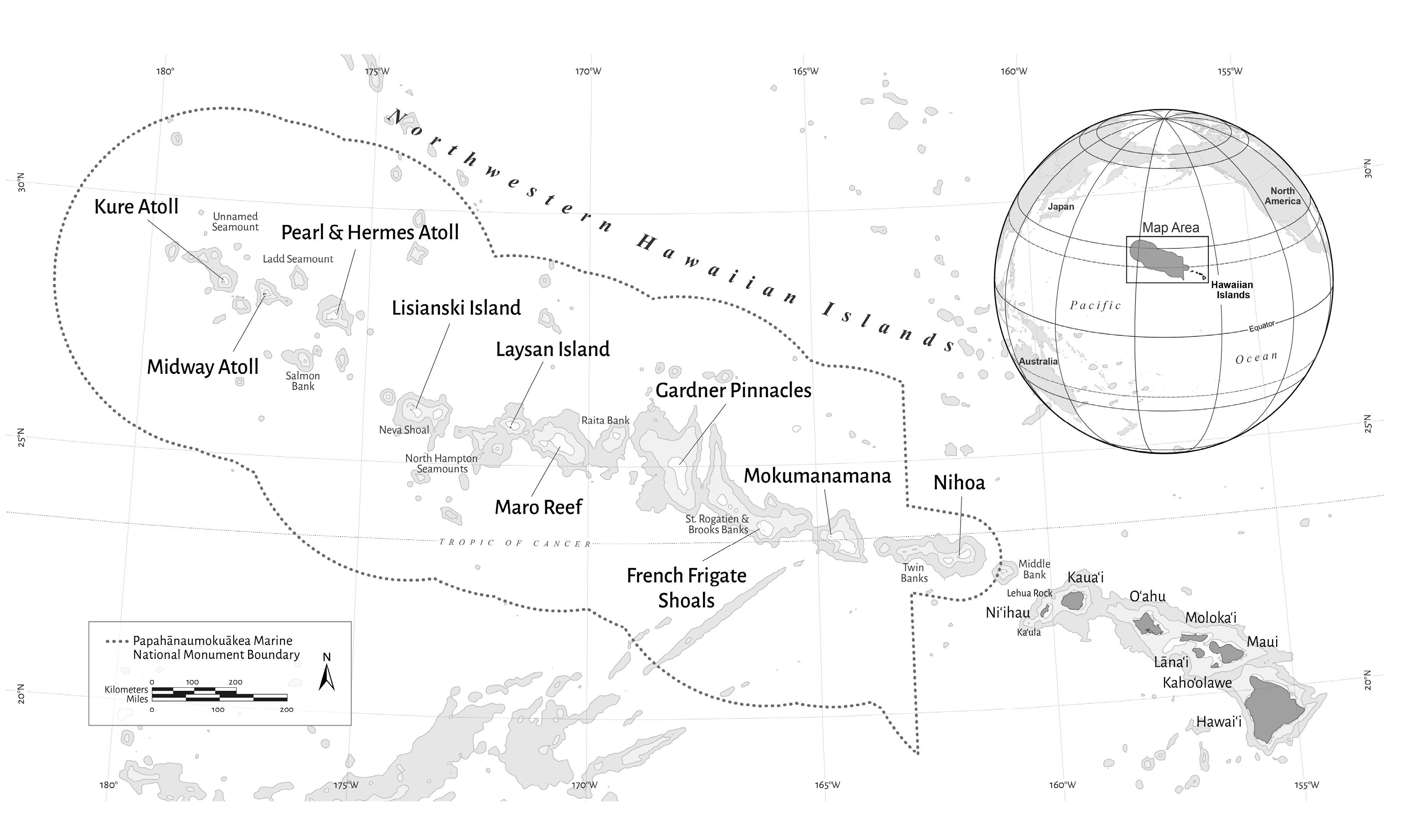
Figure 1. Map of the Hawaiian Archipelago, including the Northwestern Hawaiian Islands (NWHI). The boundary of Papahānaumokuākea Marine National Monument is shown by the dotted line.
Diversity 12 00430 g001
Figure 2. Conditional effect plots for (a) the standardized mean VRM deviation at 4-cm resolution and (b) the interaction between the standardized mean VRM at 1-cm resolution and the standardized curvature range showing the estimates of species richness per survey site.
Diversity 12 00430 g002
Figure 3. Conditional effect plots for (a) the standardized mean VRM deviation at 4-cm resolution and (b) the interaction between the standardized mean VRM at 1-cm resolution and the standardized curvature range showing the estimates of herbivore abundance per survey site.
Diversity 12 00430 g003
Figure 4. Conditional effect plots for (a) the standardized mean VRM at 1-cm resolution, (b) the standardized mean VRM deviation at 4-cm resolution, (c) the proportion of Acropora coral cover and (d) the proportion of Pocillopora coral cover showing the estimates of corallivore abundance per survey site.
Diversity 12 00430 g004
Figure 5. Conditional effect plots for (a) the standardized mean VRM at 1-cm deviation, (b) the standardized mean VRM deviation at 4-cm resolution and (c) the standardized curvature range showing the estimates of piscivore abundance per survey site.
Diversity 12 00430 g005
Figure 6. Ordination generated by distance-based redundancy analysis (dbRDA) for the fitted model of the fish data from the 80 survey sites based on Bray-Curtis dissimilarity after square-root transformation of fish abundance versus the five explanatory variables: geographical locations (island/atoll names with “(loc)”), depth, standardized mean VRM at 1-cm resolution (VRM 1 cm), standardized mean VRM deviation at 4-cm resolution (VRM 4 cm) and standardized curvature range (curvature range). The strengths of the relationships between each explanatory variable and the dbRDA axes (dbRDA1 and dbRDA2) are shown as vectors at the top right. The abundances of the five fish species (A–E) are shown by the sizes of pies. The range fish abundance after square-root transformation is shown for each species in the parentheses next to the species name on the bottom right of the figure.
Diversity 12 00430 g006
Table 1. Results of DISTLM conditional tests for the structure of fish assemblages as a whole on the basis of Bray-Curtis dissimilarity after square-root transformation of fish abundance. Explanatory variables used were geographical locations, depth, standardized mean VRM at 1-cm resolution, standardized mean VRM deviation at 4-cm resolution and standardized curvature range. None of the benthic cover variables further improved the model on the basis of AICc. The “+” in the variables column denotes an addition of the explanatory variable to the model.
VariablesExplained SSPseudo-FPR2
location42,4744.6500.00020.239
+depth16,72010.3020.00020.333
+standardized VRM 1 cm36802.3080.00600.354
+standardized VRM deviation 4 cm10,5977.2210.00020.414
+standardized curvature range32022.2200.00260.432
Publisher’s Note: MDPI stays neutral with regard to jurisdictional claims in published maps and institutional affiliations.