Zooplankton Community Response to Seasonal Hypoxia: A Test of Three Hypotheses

Abstract

Several hypotheses of how zooplankton communities respond to coastal hypoxia have been put forward in the literature over the past few decades. We explored three of those that are focused on how zooplankton composition or biomass is affected by seasonal hypoxia using data collected over two summers in Hood Canal, a seasonally-hypoxic sub-basin of Puget Sound, Washington. We conducted hydrographic profiles and zooplankton net tows at four stations, from a region in the south that annually experiences moderate hypoxia to a region in the north where oxygen remains above hypoxic levels. The specific hypotheses tested were that low oxygen leads to: (1) increased dominance of gelatinous relative to crustacean zooplankton, (2) increased dominance of cyclopoid copepods relative to calanoid copepods, and (3) overall decreased zooplankton abundance and biomass at hypoxic sites compared to where oxygen levels are high. Additionally, we examined whether the temporal stability of community structure was decreased by hypoxia. We found evidence of a shift toward more gelatinous zooplankton and lower total zooplankton abundance and biomass at hypoxic sites, but no clear increase in the dominance of cyclopoid relative to calanoid copepods. We also found the lowest variance in community structure at the most hypoxic site, in contrast to our prediction. Hypoxia can fundamentally alter marine ecosystems, but the impacts differ among systems.

1. Introduction

Hypoxia (dissolved oxygen levels ≤ 2 mg/L) can be a significant stressor to marine organisms and ecosystems, resulting in changes in communities through direct mortality of individuals or lower population growth of sensitive species concurrent with increased dominance of less sensitive species. In some seasonally hypoxic systems, particularly many estuaries, studies have shown important effects of hypoxia on individual species, community composition, and biogeochemical cycles that have been exacerbated by anthropogenic nutrient inputs and global climate change [1]. However, in taxonomically diverse systems that experience moderate or intermittent hypoxia, some species may respond strongly to conditions, but the overall effect on communities is less clear. Many coastal regions world-wide currently fall into this category of what may be classified as moderately or episodically stressed, at least from the perspective of pelagic organisms that can move to avoid near-bottom oxygen depletion.

From studies that have focused on the effects of hypoxia on zooplankton, several themes have developed in the literature, some with more evidential support than others. There is clear evidence of direct effects of hypoxia on reproduction and survival of zooplankton when oxygen levels decline below critical, species-specific thresholds, e.g., [2,3,4,5,6,7]. Indirect effects of hypoxia have also been demonstrated, primarily acting through altered distributions which can increase encounter rates among predators and prey when both avoid hypoxic conditions [8,9,10], or decrease encounters when the hypoxia is used as a predation refuge [11,12,13]. Through time, these direct and indirect effects may depress populations or lead to shifts in species dominance such that the structure and productivity of communities are altered [14,15]. Perhaps because of the difficulty in studying these processes in the field, there is little evidence of indirect, community-level effects on zooplankton in the literature to date.

In this study, we examine three hypotheses of how seasonal hypoxia alters zooplankton communities and explore a more general hypothesis about the effects of stressors on the temporal stability of species diversity and community structure. The first hypothesis we address is that, over time, hypoxia causes a shift in dominance from crustacean zooplankton toward an increased dominance by gelatinous zooplankton. This shift has been suggested in the literature, e.g., [16,17,18], and theorized to result from the relative tolerance of gelatinous taxa to low oxygen [16,19,20] and related shifts in their predator–prey interactions [21,22]. A shift to greater dominance of gelatinous zooplankton would have large consequences to food webs and the production of upper trophic level organisms since gelatinous zooplankton are not high-quality prey for most consumers and can be predators on their early life stages or competitors for their prey [23]. Here, we address this hypothesis by comparing the ratio of gelatinous to crustacean zooplankton among stations and months, with the hypothesis that the ratio will increase when and where hypoxia is most intense.

The second hypothesis that we address is that regions exposed to hypoxia will have a higher dominance of cyclopoid copepods relative to calanoid copepods. This potential shift has been hypothesized based on the differing physiology of the organisms, primarily focusing on broadly distributed cyclopoid copepods, Oithona spp., compared to dominant calanoid copepods. Cyclopoid copepods have been hypothesized to be competitively superior to calanoid copepods in low oxygen conditions due to their relatively small body size (i.e., high surface area to volume ratio, which could enhance oxygen uptake), low metabolism and hence, oxygen demand [2,24,25]. It has been shown that cyclopoids have overall lower metabolism due to their lower swimming behavior than calanoids [26,27]. In addition, many calanoid copepods free-spawn their eggs into the water column, where those that are negatively buoyant may sink into deeper, oxygen-depleted waters before hatching, thus decreasing their viability. In contrast, cyclopoid copepods typically carry their eggs in brood sacs, so could protect their eggs from hypoxia by remaining in well-oxygenated water until they hatch [2]. Here, we address this hypothesis by comparing the ratio of cyclopoid to calanoid copepods among stations and months, with the hypothesis that a higher ratio of cyclopoids will be present when and where hypoxia is most intense.

The third hypothesis we address is that over time, hypoxia leads to an overall decline in zooplankton abundance and biomass. Zooplankton may decrease through a combination of direct effects on growth, survival, or reproduction, or through trophic effects if their feeding is affected by conditions, their ability to avoid predators is reduced, or predator encounters are increased. Evidence of decreased zooplankton abundances during hypoxia has been shown in several systems including the Chesapeake Bay [8] and Gulf of Mexico [28].

Lastly, we examine whether higher variance in community structure, including less stable seasonal cycles and bigger differences among years, occurs at sites that experience hypoxia compared to unstressed sites. This hypothesis was based on evidence that degraded habitats exhibit higher community variance than healthy habitats, e.g., [29]. We hypothesized that the zooplankton community that inhabits more hypoxic sites would be less stable over time than at sites with higher oxygen levels.

We addressed these hypotheses using data collected over two years at stations that lie along a gradient of oxygen conditions in Hood Canal, a seasonally hypoxic sub-basin of Puget Sound, Washington. Hood Canal is a glacially-carved fjord with a shallow sill at the northern end that restricts deep water exchange with the ocean. High primary production, stratification, and long water residence times in the southern end of the basin lead to oxygen drawdown through summer and hypoxia in southern regions while oxygen levels remain relatively high in the north. Residence times in southern Hood Canal are ~73 days sub-pycnocline, and ~15 days for surface water; in the north, they are ~15 and 8 days for deep and surface layers, respectively [30]. Southern Hood Canal has naturally experienced seasonal hypoxia for hundreds of years [31], with the persistence and intensity of hypoxia varying annually. Oxygen is chronically low at the head of the canal near Lynch Cove; hypoxic for 2–6 months per year at other sites in southern Hood Canal; and, in some years, southerly wind bursts lead to rapid upwelling of hypoxic deep waters, episodically exposing the entire water column to hypoxia and resulting in fish kills [32]. The northern region of Hood Canal, which is typically unaffected by hypoxia, provides a natural contrast in the conditions experienced by resident zooplankton communities in an otherwise similar environment.

2. Methods

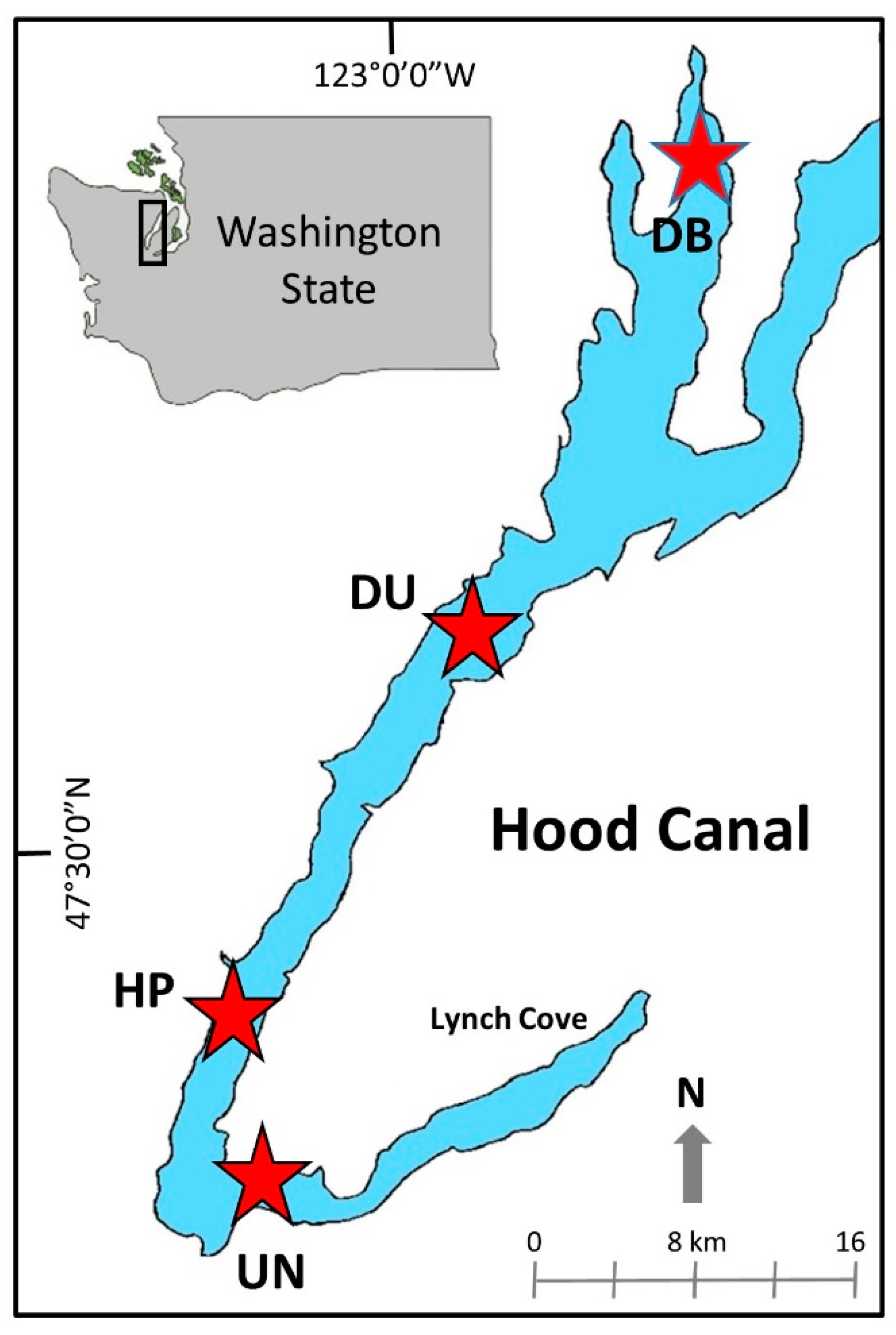
2.1. Field Collections

We conducted monthly cruises from June to October in 2012 and 2013 from the University of Washington’s R/V Clifford A. Barnes as part of a larger program which also conducted midwater trawls and bioacoustics to study fish and macrozooplankton responses to hypoxia. We sampled four stations that lie along the north–south gradient in oxygen in Hood Canal (Figure 1). Of these four stations, two were relatively shallow: Dabob Bay (DB) 65–90 m and Union (UN) 55–70 m. The other two were relatively deep: Duckabush (DU) 150–165 m and Hoodsport (HP) 100–115 m. Because station depth can be an important factor controlling species composition and abundances independent of other environmental variables, we focused our comparisons on the pairs of stations with similar water depth but different oxygen conditions—DB (shallow, not hypoxic) versus UN (shallow, hypoxic), DU (deep, not hypoxic) versus HP (deep, hypoxic).

To characterize the water properties (temperature, salinity, fluorescence, and oxygen), we conducted Conductivity-Temperature-Depth (CTD) profiles using a Sea-Bird Electronics SBE 911plus CTD equipped with a Niskin rosette, a WET Labs ECO-AFL/FL fluorometer, and an SBE 43 dissolved oxygen (DO) sensor calibrated on cruises using the modified Winkler titration method [33,34]. Zooplankton were collected using oblique tows of a 0.25 m² HydroBios MultiNet (five-net capacity) equipped with inner and outer flow meters to measure the water volume filtered and monitor for clogging. Two mesh sizes were used: 200 µm mesh nets towed at ~0.5–1 m/s to sample small, weakly motile taxa, and 335 µm mesh nets towed at 1.5–2 m/s to sample the larger, stronger swimming taxa in an identical re-cast of the tow. Replicate samples were collected in day (defined as one hour after sunrise to one hour before sunset) and night (one hour after sunset to one hour before sunrise). One set of samples from 200 µm nets was analyzed from either day or night whereas only nighttime 335 µm net samples were analyzed to minimize issues with net avoidance. All tows were conducted through the full water column to within 10 m of the bottom. Very little suggestion of net feeding was observed, so no effort was made to adjust for it. Samples were preserved in 5% buffered formalin in seawater and returned to the laboratory for analysis. For this study, full-water-column net tows from each mesh size, station, month, and year were analyzed to create a set of 40 community composition observations representing each station–month–year combination.

2.2. Laboratory Analysis

In the laboratory, samples were microscopically examined for taxonomic composition and abundance. Amphipods; crab and shrimp larvae; euphausiid furcilia and older stages; mysids; chaetognaths >1 mm length; isopods; and adult polychaetes were identified and measured in the 335 µm samples. All other organisms including gelatinous zooplankton were analyzed in 200 µm samples. Data from the two mesh sizes were combined to form “full community” data. Samples collected using 335 µm nets were first sorted on a light table for large, easily visible organisms. The sample was then split with a Folsom splitter to a fraction that contained approximately 100 total organisms of the target taxa and all of these organisms were analyzed. Samples collected using 200 µm nets were quantitatively subsampled with Stempel pipettes for small organisms, except gelatinous zooplankton which were identified and measured from the whole sample or Folsom splits. Copepods, euphausiids, shrimp larvae, pteropods, medusae, ctenophores, siphonophores, and amphipods were identified to species and life history stage; a few species that are difficult to discriminate were identified to genus. Some taxa were identified to higher groups (e.g., trochophores, chaetognaths, barnacles, bivalves) and not separated by life stage. Ichthyoplankton and all eggs and nauplii except barnacles were excluded from analyses.

The density of organisms (number of individuals m⁻³) was calculated from sample counts using the volume of water each net filtered. Biomass (in carbon weight) of measured taxa was calculated from densities using length:weight relationships reported in the literature, e.g., [35,36,37,38], and, for unmeasured organisms, from carbon conversions by species and life stage taken from the literature (e.g., [39,40]). Full water column abundance (the number of individuals present per m²) and full water column biomass (mg carbon m⁻²) of each organism was calculated by multiplying the densities and biomass densities by the depth of the net tow. We report numbers per m² herein to represent the populations present at each site, independent of station depth.

2.3. Statistical Analyses

We used distance measures and ordination to test the hypothesis that hypoxia affected community stability, defined as higher variance in composition over time. A data matrix consisting of 40 samples × 56 taxa was constructed by summing across all life stages of each species in each sample. Variance in community structure was assessed using a matrix of Bray–Curtis distance (dissimilarity) measures calculated between each pair of samples as 1 − (ΣMIN_A,B/(ΣA + ΣB)), where ΣMIN_A,B is the sum of the lesser values of the abundance of all species in samples A and B (i.e., the sum of the shared abundances); ΣA and ΣB are the total abundance of zooplankton in each of the two samples. The average distance and variance in distance at each site were calculated as: (1) the average of distances calculated between all samples collected at a station within each year; (2) the variance in distances between all sample pairs in both years at a station.

A non-metric multidimensional scaling (NMDS) ordination run on the distance matrix was used to visualize whether a more regular seasonal cycle and lower difference between years occurred at non-hypoxic sites compared to hypoxic sites. Prior to ordination, rare species (defined as those occurring in <10% of samples) were removed and data were Log10(Y + 0.001) + 3 transformed to normalize variances prior to analysis. The use of (Y + 0.001) + 3 rather than (Y + 1) helped prevent distorting the relationship between zeros and small non-zero values in the dataset [41]. A two-way factorial (Station and Year) permutational multivariate analysis of variance (PerMANOVA) was then run on the distance matrix to test for significant differences among sites and years by testing whether the centroids of the clusters of samples differed. Two pairwise comparisons were conducted following PerMANOVA to further test whether the centroid of communities significantly differed between station pairs: DB and UN, DU and HP. Distance measures were calculated, and NMDS ordination was conducted, in PC-ORD 7.06 [41,42].

3. Results

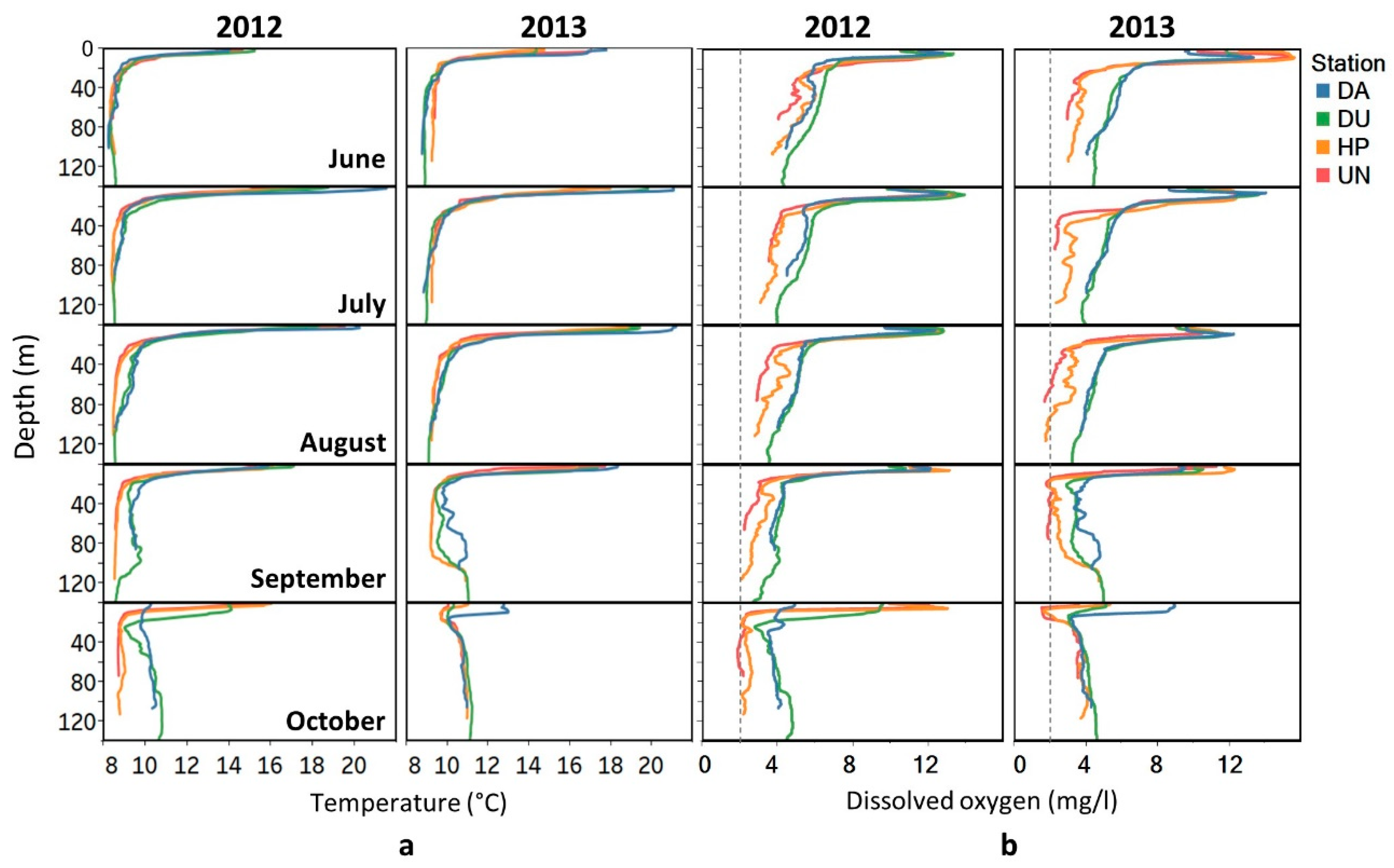
3.1. Environmental Conditions

Overall, temperatures ranged from 8.3–21.8 °C, with strong thermoclines across the upper 10–20 m through summer at all stations (Figure 2). Temperatures were 0.5–1.0 °C cooler through most of the water column in 2012 than 2013. Surface temperatures were highest in July and August each year, and were often highest at DB, but showed no consistent pattern among other stations. Deep water was typically 8–10 °C until intrusions of dense, warmer ocean water or wind-mixing warmed deep waters in fall. Deep waters were typically warmer at the northern stations than in the south, particularly following the deep-water intrusions, by up to 1.3 °C difference in October 2012.

Oxygen concentrations showed a typical seasonal cycle of declining oxygen through summer, with the lowest oxygen at the two southern stations of Union (UN) and Hoodsport (HP) compared to Duckabush (DU) and Dabob Bay (DB) (Figure 2). Oxygen mostly remained well above 4 mg/L at the two northern stations, but in late summer, much of the water column was below 4 mg/L at the southern stations, with hypoxia (≤2 mg/L) occurring in late summer at UN and, to a lesser extent, HP. Oxygen was highly variable with depth rather than monotonically decreasing, particularly in late summer or fall after the intrusion of dense ocean water into Hood Canal displaced cooler, lower oxygen water upwards, resulting in near-surface oxygen minimum layers. This displacement was evident earlier in the north, and began later in 2012 (October) than 2013 (September).

Chlorophyll peaks were typically found in the upper 10 m, at the base of the shallow pycnoclines (Figure S1). In 2012, chlorophyll was moderately low (~10 µg/L) and similar at all stations until larger peaks (~30 µg/L) at UN and HP in September and October. In 2013, chlorophyll was much higher at UN and HP in June and September, reaching 40 µg/L in September.

3.2. Zooplankton Community Composition

Calanoid copepods dominated the zooplankton abundance. In order of abundance, the dominant calanoid copepods were Paracalanus sp., Metridia pacifica, Calanus (mostly C. pacificus but also some C. marshallae), Pseudocalanus (primarily P. newmani but also P. moultoni and P. minutus), Microcalanus spp., Centropages sp., Acartia hudsonica, Aetideus spp., and Paraeuchaeta elongata. The cyclopoid copepods Oithona similis, O. atlantica, Oncaeidae, and Ditrichocoryceaus anglicus (previously called Corycaeus anglicus) all occurred in our study area, with Oithona similis vastly dominating the cyclopoid copepod abundance as is common in many regions of the world’s oceans. Other dominant crustacean zooplankton were amphipods (Primno macropa, Parathemisto pacifica, Cyphocaris challengeri), decapod larvae (Fabia subquadrata, Metacarcinus magister, Glebocarcinus oregonensis, Lophopanopeus bellus, Pugettia spp., and others), Neotrypaea californiensis, euphausiids (Euphausia pacifica, Thysanoessa raschii, T. spinifera), cladocerans (Evadne and Podon), ostracods, and barnacle nauplii.

Fifteen jellyfish genera were identified in MultiNet samples: three scyphozoans, nine hydrozoans, two siphonophores, and one ctenophore. The calycophoran siphonophore Muggiaea atlantica dominated the abundance and biomass of the gelatinous zooplankton. Other important taxa were the hydromedusae Obelia sp., Aglantha digitale, Clytia gregaria, Proboscidactyla flavicirrata, Euphysa sp., and Leuckartiara sp. Gelatinous zooplankton patterns from these cruises are reported in [43].

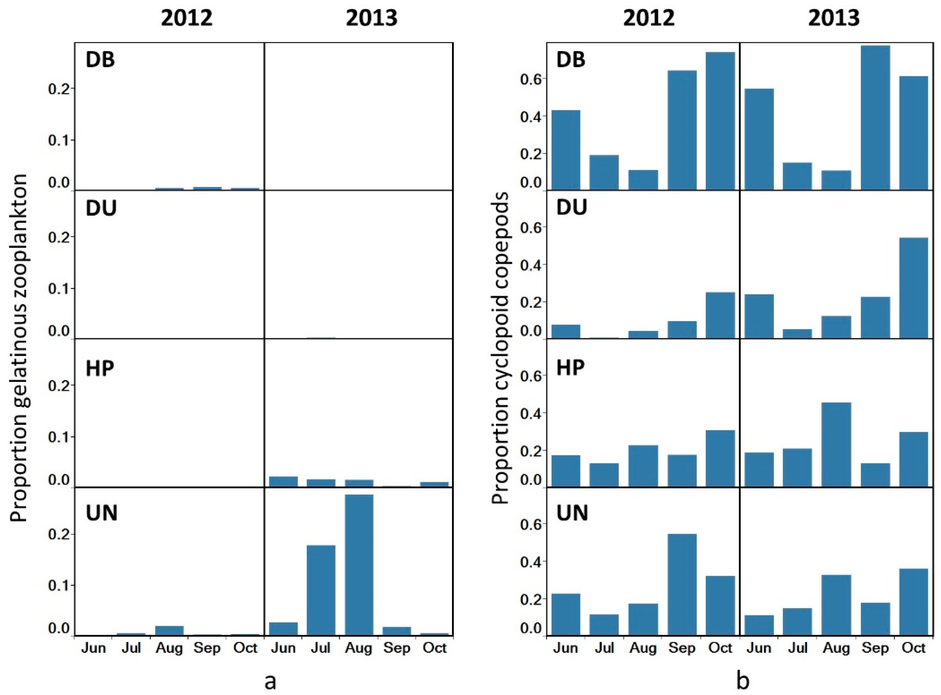
3.3. Species Dominance

Gelatinous zooplankton comprised a fairly small component of the zooplankton biomass overall; crustacean taxa dominated the biomass at all times (Figure 3a). The ratio between gelatinous and crustacean zooplankton biomass was higher in the south than at the northern sites, particularly at the most hypoxic site (UN), and was higher in 2013 than 2012. In August 2013, the ratio reached a high of 0.39. All of the dominant gelatinous species were more abundant at the southern stations (UN and HP) than in the north, and in 2013 compared to 2012 (Figure S2); two taxa (Rathkea sp. and Obelia sp.) were exclusively found at southern stations.

The ratio of cyclopoid to calanoid copepods was higher at DB than at UN and higher at HP than DU (Figure 3b). The ratio showed a seasonal cycle with higher dominance of cyclopoids in fall, particularly at the two northern stations. There was little change in the ratio between years.

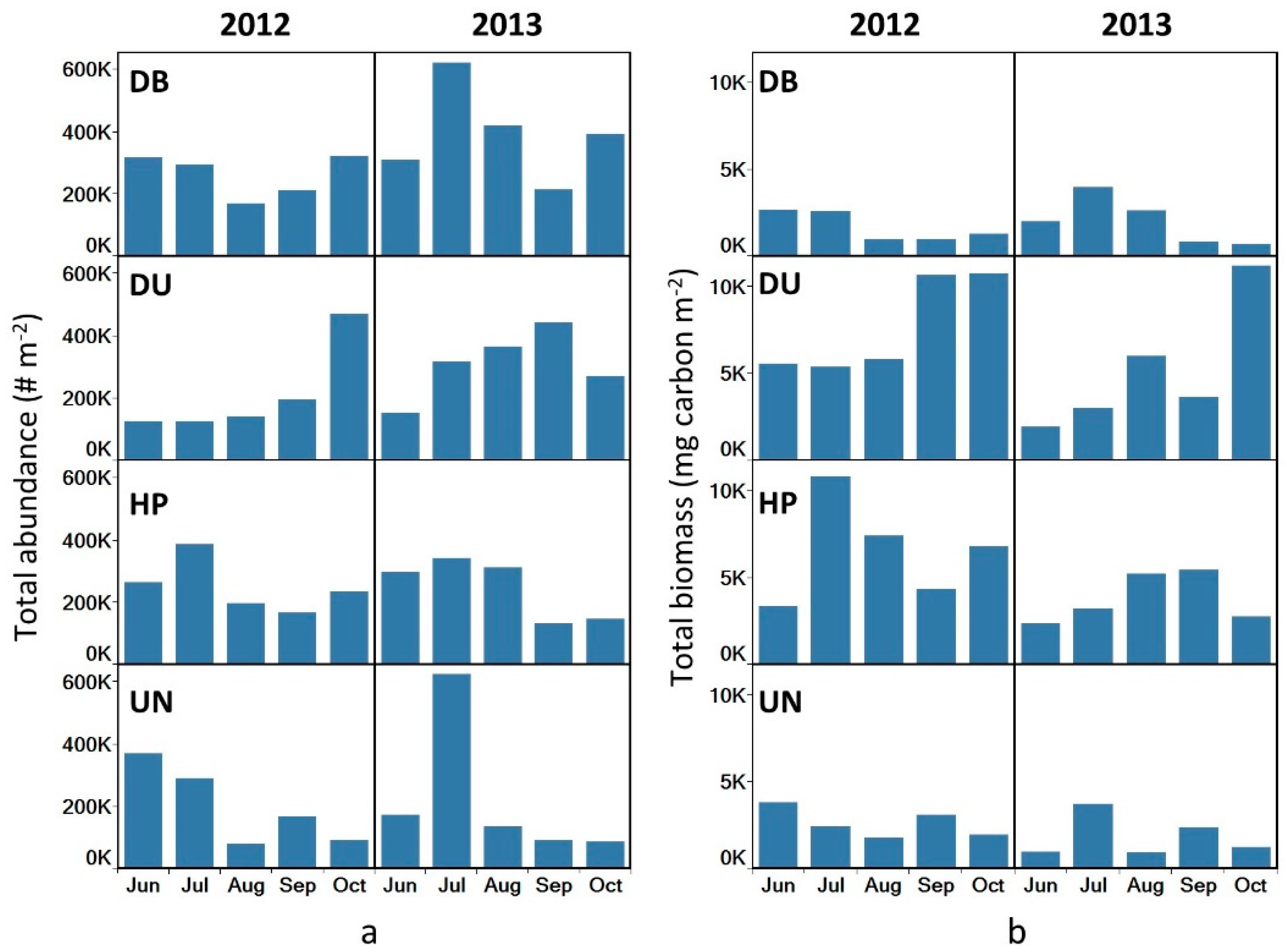
3.4. Total Abundance and Biomass

Overall, total zooplankton abundance (number of individuals m⁻²) was lowest at UN, particularly late in the season in both years, with a notable exception of July 2013 (Figure 4). Abundance was highest overall at DB. Abundances were lower in most months at DU than at HP in 2012, but higher in 2013. The seasonal cycle of abundance differed among stations: abundances dropped from early summer to autumn at UN and to a lesser extent HP, whereas they increased through summer to fall at DU and were variable at DB.

Biomass patterns differed from abundances: biomass was very low at both of the shallower stations, DB and UN, compared to DU and HP, indicating substantial differences in size-composition among stations with larger taxa comprising the community at HP and DU compared to UN and (especially) DB. Total biomass generally declined over each season at DB and UN, increased in late summer or fall at DU, and differed in pattern between 2012 and 2013 at HP.

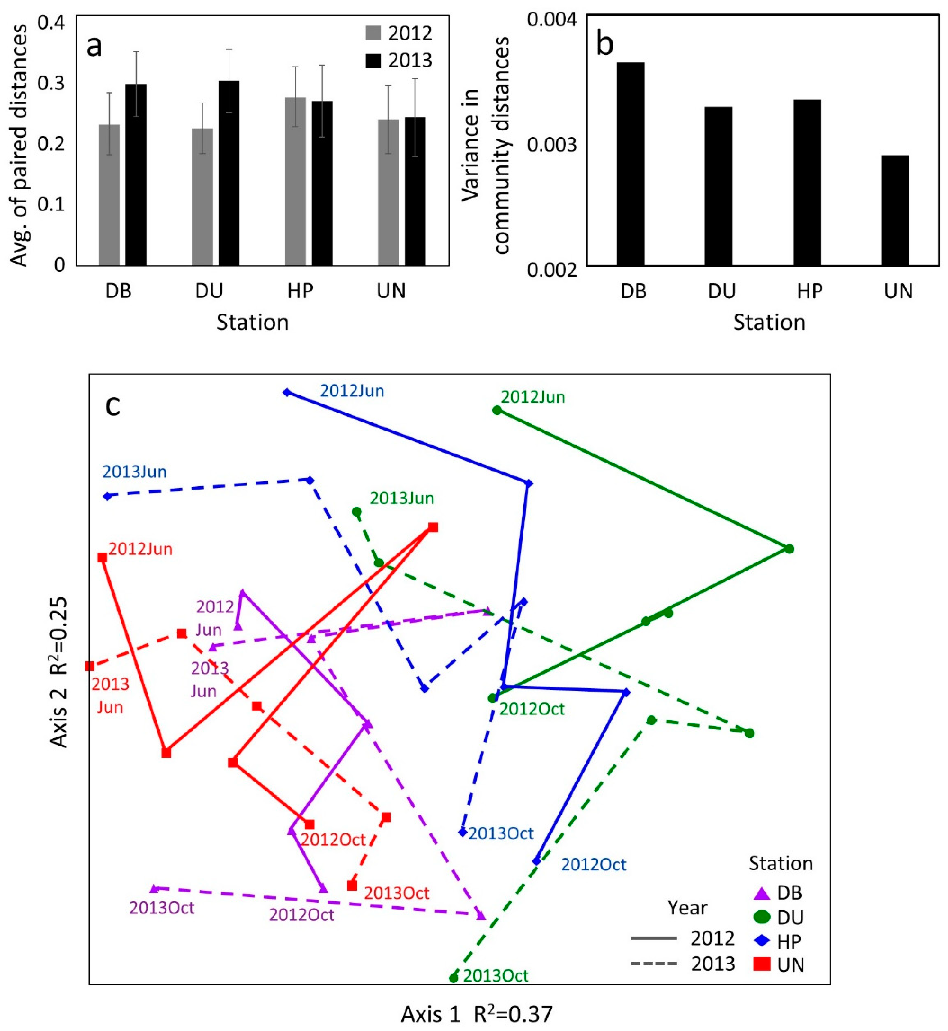
3.5. Zooplankton Community Stability

Distance metrics showed no clear pattern of greater variance in community structure between the northern, less-hypoxic and southern, more-hypoxic stations when examining average distances within each year (Figure 5a). In 2012, DB, DU, and UN all had very similar average dissimilarity values. In 2013, the two northern stations had slightly higher average distance metrics than the southern stations, but the differences were not significant. When calculated as the overall variance in community dissimilarity across all possible date pairs in both years (Figure 5b), the variance in community distances was lowest at the most hypoxic site, UN, highest at DB, and did not differ between DU and HP.

A three-dimensional NMDS ordination explained 81.4% of the original variance in distances among samples: Axes 1, 2, and 3 carried 36.6%, 24.9%, and 19.9% of the variance, respectively. Zooplankton communities showed a shift among stations along Axis 1, ordered from left to right as UN, DB, HP, and DU (Figure 5c). Of the two shallower stations, UN and DB, the more hypoxic UN fell to the left of DB; also, of the two deeper stations, the more hypoxic HP fell to the left of DU. No large overall difference in communities was noted between 2012 and the more hypoxic year, 2013; there was a small shift in communities to the left along Axis 1 from 2012 to 2013 but, except at HP, the shift was not consistent in every month. Taxa that were most strongly positively correlated with Axis 1 (i.e., were more abundant in samples to the right in the plot) were the gammarid amphipod Cyphocaris challengeri (r = 0.48) and the shrimp Pasiphaea pacifica (r = 0.54); negatively correlated were the hydrozoan Proboscidactyla flavicirrata (r = −0.67), Paguridae decapod larvae (r = −0.64), unspeciated shrimp larvae (r = −0.64), unspeciated polychaete larvae (r = −0.61), Fabia subquadrata crab larvae (r = 0.60), and bryozoan cyphonauts (r = −0.60).

The position of samples along Axis 2 primarily reflected seasonal patterns in community composition. Within each station, sample dates descended along Axis 2 from early to late each year. Taxa that were most strongly positively correlated with Axis 2 (i.e., were more abundant in samples toward the top of the plot) were the euphausiid Euphausia pacifica (r = 0.66), amphipod Themisto pacifica (r = 0.60), copepod Centropages abdominalis (r = 0.59), and Cancridae crab larvae (r = 0.59); strongest negative correlations were with the copepod Aetideus sp. (r = −0.49), the jellyfish Euphysa sp. (r = −0.48), and the larvacean Oikopleura dioeca (r = −0.47).

PerMANOVA results indicated that community composition significantly differed among stations (F = 3.86, p = 0.0002) and subsequent pairwise comparisons showed that communities at DB significantly differed from UN (t = 1.47, p = 0.013) and DU significantly differed from HP (t = 1.61, p = 0.010). PerMANOVA results also indicated that communities in 2012 significantly differed from 2013 (F = 2.39, p = 0.018). There was no significant interaction between Year and Station (F = 1.31, p = 0.15).

4. Discussion

Of the three hypotheses on zooplankton community response to hypoxia we explored—that where oxygen is low, gelatinous zooplankton increase in dominance relative to crustacean zooplankton, cyclopoid copepods increase relative to calanoids, and total zooplankton abundances and biomass decrease—we found support for an increased dominance of gelatinous zooplankton and decreased total zooplankton abundance and biomass, but we found no clear shift towards increased dominance of cyclopoid copepods relative to calanoid copepods. We also found differences in community structure among sites, but the temporal variance in community structure was lowest at the most hypoxic site, rather than higher as we had predicted.

4.1. Species Dominance

4.1.1. Gelatinous vs. Crustacean Zooplankton

A growing number of studies have reported increases in gelatinous zooplankton in eutrophied and otherwise stressed coastal waters, reviewed in [44,45]. Eutrophied systems are commonly more turbid and have smaller size-composition of zooplankton [14,46,47], both of which could favor non-visual predators such as jellyfish over fish in competition for prey. Differences in relative susceptibility to oxygen—particularly effects on movement and escape responses—can shift predator–prey interactions in favor of jellyfish predators over their prey [21,48]. Furthermore, jellyfish reproduction can become more successful in low DO bottom-water where there is less benthic competition for space for eggs (planula) to settle [49]. While most attention has been paid to increases in large, highly visible scyphozoan medusae, increases in siphonophores and tiny hydromedusae that are not in the public eye can have equally significant impacts on ecosystems through changes in food webs. These taxa are more abundant and more diverse, if lower in biomass, than scyphomedusae.

The siphonophore Muggaiea atlantica vastly dominated the gelatinous zooplankton biomass, reaching peak densities >1500 Ind m⁻³ of nectophores and bracts combined. Of 12 species of gelatinous zooplankton from Puget Sound measured for oxygen consumption [19], it was reported as having one of the highest rates (0.7 umol g wet weight⁻¹ h⁻¹) but the lowest critical oxygen partial pressure (P_crit ~5 hPa = ~0.2 mg/L at 10 °C and 30 psu). P_crit—the oxygen level below which oxygen uptake can no longer be regulated and metabolism dramatically decreases [50]—is a good indicator of the level of oxygen a species can tolerate well. This indicates that M. atlantica is well adapted to the typical oxygen levels in Hood Canal. Below its critical oxygen level, M. atlantica quickly suffers high mortality [19], but since it does not have a benthic life stage that would be exposed to severely hypoxic bottom waters, it could remain in surface waters and rarely experience oxygen that low. M. atlantica’s prey base ranges from microzooplankton to fish eggs, but is primarily copepods; with predation rates estimated at 5–10 prey colony⁻¹ d⁻¹ [51], they can exert large predation pressure on zooplankton populations when their abundances are high [19]. These high predation rates may ultimately increase hypoxia if the consumption of zooplankton reduces grazing of phytoplankton [52].

Our net tows did not adequately sample the largest gelatinous taxa, some of which can reach >1 m diameter, but sampling conducted concurrent to ours estimated their biomass using semi-quantitative mid-water trawls. Aequorea victoria—the largest hydrozoan in Hood Canal—dominated the abundances of these large jellyfish, while the larger scyphozoan taxa Cyanea capillata and Phacellophora camtschatica dominated the total biomass. Like the smaller taxa, all of the large species except Cyanea were also found in higher biomass at the southern stations and declined throughout the summer; their overall biomass was higher in 2013 than 2012 [53]. Cyanea capillata, Phacellophora camtschatica, and Aurelia labiata are all known to have high tolerance for low oxygen conferred by their ability to store oxygen in their interstitial gel [20].

4.1.2. Cyclopoid vs. Calanoid Dominance

Several functional trait differences between cyclopoid and calanoid copepods have been posed as explanations for the relative success of cyclopoids under low oxygen conditions. Lower metabolic demands of cyclopoid copepods compared to calanoids has been suggested, partially based on observations that Oithona—arguably the most abundant cyclopoid in the world’s oceans [54]—has a stealth, sit-and-wait feeding style to detect motile prey whereas many calanoid copepods actively generate feeding currents and swim more continuously to encounter non-motile prey [55]. Paffenhoffer [56] found that Oithona plumifera spent only 9% of the time moving compared to the calanoid copepods Paracalanus spp. which moved 80% of the time. This low activity also would serve to hydrodynamically hide Oithona, which may be particularly advantageous if copepods and visual predators must both move towards surface to avoid hypoxia. More recently, studies have quantified O. similis respiration, finding it to be as much as 8X lower than equivalently sized calanoid copepods [25]; and that they are smaller body size than most calanoids also indicates a higher tolerance for low oxygen [57]. Uye [14] reported that cyclopoid copepods dominated a eutrophied, hypoxic estuary in Japan, hypothesizing that the females, which carry brood sacs, could protect their eggs from deep hypoxic water whereas many calanoids broadcast spawn eggs which could sink into hypoxic water before hatching. Through this processes, cyclopoids could increase relative to calanoids after only 1–2 generations.

Together, these traits led to the hypothesis that cyclopoids would be relatively more dominant at the hypoxic, southern regions of Hood Canal compared to northern regions—a hypothesis that was not supported in this study. Not only were Oithona a lower portion of the copepods at the southern stations, but they also showed only moderately increased importance in fall at UN and HP relative to large increases at DU and DB. A previous study in southern Hood Canal [10] reported an increase in dominance of O. similis in autumn when hypoxia was most intense, but that study did not sample contrasting, higher oxygen regions to the north to provide context for the change. O. similis feed preferentially on ciliates but can switch to detritus and alternative prey to maintain year-round reproduction, at least in some ecosystems [58]; their egg production rate is fairly low compared to calanoids [59] but can be maintained through fall and winter when other copepod egg production declines [60,61]. Due to Oithona’s small size, larval but not juvenile fish prey upon them, so Oithona is also likely to experience relief from its vertebrate predators as the season progresses. These different mechanisms for Oithona’s seasonally-increased dominance cannot be separated in this study so remain to be explored. Since the opposite patterns were observed than predicted, perhaps in our study years, hypoxia was not severe or persistent enough to affect populations over multiple generations.

4.2. Abundances and Biomass

A negative effect of hypoxia on total biomass and abundances is the most common effect on zooplankton reported in the literature, e.g., [2,8,47], but that has not always been the finding, e.g., [13,62], and considerable species-level differences have been reported [10]. Some taxa such as polychaete larvae are negatively associated with oxygen, i.e., more abundant during hypoxia, and are found directly within hypoxic water [10,63]. Elliott et al. [28] found overall lower abundances of some zooplankton in the Gulf of Mexico when a greater portion of the water column was hypoxic, but abundances of some larger zooplankton increased with the vertical extent of hypoxia until 60% the water column was hypoxic. In parallel studies to this one, Sato et al. [64] found no relationship between oxygen and acoustically-measured adult and juvenile euphausiid biomass, whereas Li et al. [65] found that euphausiid early life stage abundances were negatively affected by DO compared to older stages.

We found decreased abundances, particularly at UN, despite overall higher chlorophyll levels at the southern stations. This impact on zooplankton has clear implications for growth and survival of their predators, perhaps most critically for fish larvae, which are highly dependent on prey availability [66]. Decreased abundances and biomass are likely to result in decreased trophic energy transfer unless avoidance of hypoxic waters increases overlap with predators [67,68]. In our system, evidence for changes in predator–prey overlap is mixed: Sato et al. [64] found no hypoxia-driven change in fish or macro-zooplankton vertical distribution, but Keister and Tuttle [10] reported vertical shifts of several mesozooplankton species, and Parker-Stetter et al. [69] found that near-surface oxygen minimum layers can separate fish from their prey, providing a predation refuge.

4.3. Community Structure

Hypoxia can produce shifts in the structure of pelagic communities on multiple time scales, favoring taxa with greater hypoxia tolerance or those with life-history strategies that minimize exposure [70]. Species are differently impacted depending on their generation times relative to hypoxia, and their sensitivity to acute stress. On multi-year timescales, seasonally recurring hypoxia can structure the zooplankton by limiting species that cannot complete their life cycle in the region—e.g., those which are benthic as adults. For holoplankton that can have several generations during one season, hypoxia may act as a chronic stressor, slowly affecting populations through slower growth or inhibited reproduction.

In this study, we found that the differences between communities at stations that experienced hypoxia and those that did not were relatively subtle compared to seasonal changes and differences between the deeper versus shallower stations. Species relationships with Axis 1 of the NMDS ordination, along which the more hypoxic stations fell to the left (negative) relative to their paired stations, indicated that two taxa that were less common at hypoxic stations were the shrimp Pasiphaea pacifica and the gammarid amphipod Cyphocaris challengeri. However, for P. pacifica, station depth may have been more important in their pattern along Axis 1 as they were virtually absent from both of the shallower stations, DB and UN. Other decapods (Paguridae, Fabia, and some unspeciated shrimp larvae) were more common at the hypoxic stations, though whether the oxygen levels were somehow indirectly beneficial to them is not clear. Of other taxa that were also more common at the hypoxic sites, the hydrozoan Proboscidactyla flavicirrata, polychaete larvae, and siphonophore M. atlantica all have been shown to be hypoxia tolerant [10,19].

Temporally-varying stressors can cause large, or dampened, fluctuations in organism abundances depending on the degree of perturbation and the relative time scales of population dynamics versus environmental changes. In this study, we hypothesized that communities at hypoxic sites would exhibit higher temporal variability in community structure than at unstressed sites, and that this would be expressed as higher dissimilarity across months and years, and more dispersion in ordination space. This variation of the ‘Anna Karenina principle’ (AKP), developed to explain patterns in microbial assemblages, presumes that community response to a stress (in this case, hypoxia) is stochastic, resulting in many more potential structures than if undisturbed [71,72]. That we observed lower seasonal and interannual variance in community composition at sites where seasonal hypoxia occurs counters the idea that there was a stochastic nature either to the perturbations or the community response.

Overall species richness and diversity did not differ greatly between hypoxic–normoxic site pairs, so the lower community variance at hypoxic sites was not likely driven by the absence of sensitive species, nor did we find evidence of higher variance caused by lower diversity as has been reported in several studies of benthic communities [73,74]. We were not able to fully assess diversity of several meroplankton which cannot be distinguished microscopically, including bivalve larvae which were significantly less abundant at UN than at other stations. Compared to holoplankton, those taxa are more likely to be affected over multi-year time scales if their benthic stages cannot escape stressful conditions. In systems that have been recurrently and semi-predictably disturbed over decades or longer, communities may have stabilized their cycles over time rather than exhibiting extreme stochastic shifts in response to each occurrence of the disturbance. This may be the case in Hood Canal where hypoxia has been a natural part of the system since pre-industrial times [31]. Alternatively, the lower variance could indicate that the moderate hypoxia which occurred during this study was not extreme enough to cause strong shifts, or that natural seasonal cycles were less pronounced at hypoxic sites due to decreased species abundances.

5. Conclusions

Seasonally hypoxic coastal systems are not all alike, and the consequences of hypoxia to their resident zooplankton communities will depend on the species composition, intensity and extent of oxygen depletion, and historical timescale of impacts. The systems which have been best studied, particularly the Chesapeake Bay and Gulf of Mexico, have been dramatically affected by anthropogenic nutrient inputs and eutrophication; they experience strongly hypoxic to anoxic conditions most years, resulting in altered ecosystem structure and function. Other systems such as many continental shelf systems and less populated estuaries may be moderately or episodically hypoxic, perhaps increasingly so with global warming as circulation, stratification, and production change [75]. Although oxygen conditions in southern Hood Canal can reach near anoxic levels in severe years, the region more commonly experiences recurrent moderately-hypoxic conditions. In this study, we observed two of the most commonly reported effects of hypoxia on zooplankton communities—increased gelatinous zooplankton and decreased overall abundances. More intense hypoxia or a larger affected region may have resulted in larger community shifts. But it is also possible that the diverse community and historic timescales of hypoxia may modulate impacts in Hood Canal through local adaptations, e.g., via behaviors, as reported by Decker et al. [76], facilitating the maintenance of populations and communities.

References

1. Breitburg, D.; Levin, L.A.; Oschlies, A.; Grégoire, M.; Chavez, F.P.; Conley, D.J.; Garçon, V.; Gilbert, D.; Gutiérrez, D.; Isensee, K.; et al. Declining oxygen in the global ocean and coastal waters. Science 2018, 359, eaam7240. [Google Scholar] [CrossRef] [PubMed] [Green Version]
2. Roman, M.R.; Gauzens, A.L.; Rhinehart, W.K.; White, J.R. Effects of low oxygen waters on Chesapeake Bay zooplankton. Limnol. Oceanogr. 1993, 38, 1603–1614. [Google Scholar] [CrossRef]
3. Stalder, L.C.; Marcus, N.H. Zooplankton responses to hypoxia: Behavioral patterns and survival of three species of calanoid copepods. Mar. Biol. 1997, 127, 599–607. [Google Scholar] [CrossRef]
4. Miller, D.C.; Poucher, S.L.; Coiro, L. Determination of lethal dissolved oxygen levels for selected marine and estuarine fishes, crustaceans, and a bivalve. Mar. Biol. 2002, 140, 287–296. [Google Scholar]
5. Invidia, M.; Sei, S.; Gorbi, G. Survival of the copepod Acartia tonsa following egg exposure to near anoxia and to sulfide at different pH values. Mar. Ecol. Prog. Ser. 2004, 276, 187–196. [Google Scholar] [CrossRef] [Green Version]
6. Grodzins, M.A.; Ruz, P.M.; Keister, J.E. Effects of oxygen depletion on field distributions and laboratory survival of the marine copepod Calanus pacificus. J. Plankton Res. 2016, 38, 1412–1419. [Google Scholar]
7. Ruz, P.M.; Hidalgo, P.; Yáñez, S.; Escribano, R.; Keister, J.E. Egg production and hatching success of Calanus chilensis and Acartia tonsa in the northern Chile upwelling zone (23°S), Humboldt Current System. J. Mar. Syst. 2015, 148, 200–212. [Google Scholar] [CrossRef]
8. Keister, J.E.; Houde, E.D.; Breitburg, D.L. Effects of bottom-layer hypoxia on abundances and depth distributions of organisms in Patuxent River, Chesapeake Bay. Mar. Ecol. Prog. Ser. 2000, 205, 43–59. [Google Scholar] [CrossRef]
9. Pierson, J.J.; Roman, M.R.; Kimmel, D.G.; Boicourt, W.C.; Zhang, X. Quantifying changes in the vertical distribution of mesozooplankton in response to hypoxic bottom waters. J. Exp. Mar. Bio. Ecol. 2009, 381, S74–S79. [Google Scholar] [CrossRef]
10. Keister, J.E.; Tuttle, L.B. Effects of bottom-layer hypoxia on spatial distributions and community structure of mesozooplankton in a sub-estuary of Puget sound, Washington, U.S.A. Limnol. Oceanogr. 2013, 58, 667–680. [Google Scholar] [CrossRef]
11. De Robertis, A.; Eiane, K.; Rau, G. Eat and run: Anoxic feeding and subsequent aerobic recovery by Orchomene obtusus in Saanich Inlet, British Columbia, Canada. Mar. Ecol. Prog. Ser. 2001, 219, 221–227. [Google Scholar] [CrossRef]
12. Taylor, J.C.; Rand, P.S. Spatial overlap and distribution of anchovies (Anchoa spp.) and copepods in a shallow stratified estuary. Aquat. Living Resour. 2003, 16, 191–196. [Google Scholar] [CrossRef]
13. Zhang, H.; Ludsin, S.A.; Mason, D.M.; Adamack, A.T.; Brandt, S.B.; Zhang, X.; Kimmel, D.G.; Roman, M.R.; Boicourt, W.C. Hypoxia-driven changes in the behavior and spatial distribution of pelagic fish and mesozooplankton in the northern Gulf of Mexico. J. Exp. Mar. Bio. Ecol. 2009, 381, S80–S90. [Google Scholar] [CrossRef]
14. Uye, S. Replacement of large copepods by small ones with eutrophication of embayments: Cause and consequence. Hydrobiologia 1994, 292, 513–519. [Google Scholar] [CrossRef]
15. Roman, M.R.; Brandt, S.B.; Houde, E.D.; Pierson, J.J. Interactive effects of hypoxia and temperature on coastal pelagic zooplankton and fish. Front. Mar. Sci. 2019, 6, 1–18. [Google Scholar] [CrossRef] [Green Version]
16. Purcell, J.E.; Breitburg, D.L.; Decker, M.B.; Graham, W.M.; Youngbluth, M.J.; Raskoff, K.A. Pelagic Cnidarians and Ctenophores in Low Dissolved Oxygen Environments: A Review. In Coastal Hypoxia: Consequences for Living Resources and Ecosystems; American Geophyical Union: Washington, DC, USA, 2001; pp. 77–100. [Google Scholar]
17. Condon, R.H.; Decker, M.B.; Purcell, J.E. Effects of low dissolved oxygen on survival and asexual reproduction of scyphozoan polyps (Chrysaora quinquecirrha). Hydrobiologia 2001, 451, 89–95. [Google Scholar] [CrossRef]
18. Richardson, A.J.; Bakun, A.; Hays, G.C.; Gibbons, M.J. The jellyfish joyride: Causes, consequences and management responses to a more gelatinous future. Trends Ecol. Evol. 2009, 24, 312–322. [Google Scholar] [CrossRef]
19. Rutherford, L.D.; Thuesen, E.V. Metabolic performance and survival of medusae in estuarine hypoxia. Mar. Ecol. Prog. Ser. 2005, 294, 189–200. [Google Scholar] [CrossRef] [Green Version]
20. Thuesen, E.V.; Rutherford, L.D.; Brommer, P.L.; Garrison, K.; Gutowska, M.A.; Towanda, T. Intragel oxygen promotes hypoxia tolerance of scyphomedusae. J. Exp. Biol. 2005, 208, 2475–2482. [Google Scholar] [CrossRef] [Green Version]
21. Breitburg, D.L.; Loher, T.; Pacey, C.A.; Gerstein, A. Varying effects of low dissolved oxygen on trophic interactions in an estuarine food web. Ecol. Monogr. 1997, 67, 489–507. [Google Scholar] [CrossRef]
22. Decker, M.B.; Breitburg, D.L.; Purcell, J.E. Effects of low dissolved oxygen on zooplankton predation by the ctenophore Mnemiopsis leidyi. Mar. Ecol. Prog. Ser. 2004, 280, 163–172. [Google Scholar] [CrossRef]
23. Purcell, J.E.; Sturdevant, M.V. Prey selection and dietary overlap among zooplanktivorous jellyfish and juvenile fishes in Prince William Sound, Alaska. Mar. Ecol. Prog. Ser. 2001, 210, 67–83. [Google Scholar] [CrossRef] [Green Version]
24. Uye, S. Production ecology of marine planktonic copepods. Bull. Plankt. Soc. Jpn. 1984, 30, 44–55. [Google Scholar]
25. Castellani, C.; Robinson, C.; Smith, T.; Lampitt, R.S. Temperature affects respiration rate of Oithona similis. Mar. Ecol. Prog. Ser. 2005, 285, 129–135. [Google Scholar] [CrossRef]
26. Paffenhöfer, G.A. Oxygen consumption in relation to motion of marine planktonic copepods. Mar. Ecol. Prog. Ser. 2006, 317, 187–192. [Google Scholar] [CrossRef] [Green Version]
27. Almeda, R.; Alcaraz, M.; Calbet, A.; Saiz, E. Metabolic rates and carbon budget of early developmental stages of the marine cyclopoid copepod Oithona davisae. Limnol. Oceanogr. 2011, 56, 403–414. [Google Scholar] [CrossRef] [Green Version]
28. Elliott, D.T.; Pierson, J.J.; Roman, M.R. Relationship between environmental conditions and zooplankton community structure during summer hypoxia in the northern Gulf of Mexico. J. Plankton. Res. 2012, 34, 602–613. [Google Scholar] [CrossRef] [Green Version]
29. Cote, D.; Gregory, R.S.; Morris, C.J.; Newton, B.H.; Schneider, D.C. Elevated habitat quality reduces variance in fish community composition. J. Exp. Mar. Bio. Ecol. 2013, 440, 22–28. [Google Scholar] [CrossRef]
30. Babson, A.L.; Kawase, M.; MacCready, P. Seasonal and interannual variability in the circulation of Puget Sound, Washington: A box model study. Atmosphere-Ocean 2006, 44, 29–45. [Google Scholar] [CrossRef]
31. Brandenberger, J.M.; Louchouarn, P.; Crecelius, E.A. Natural and post-urbanization signatures of hypoxia in two basins of Puget Sound: Historical reconstruction of redox sensitive metals and organic matter inputs. Aquat. Geochem. 2011, 17, 645–670. [Google Scholar] [CrossRef]
32. Newton, J.; Bassin, C.; Devol, A.; Kawase, M.; Ruef, W.; Warner, M.; Hannafious, D.; Rose, R. Hypoxia in Hood Canal: An overview of status and contributing factors. In Proceedings of the 2007 Georgia Basin Puget Sound Reseach Conference, Vancouver, BC, Canada, 26–29 March 2007. [Google Scholar]
33. Carpenter, J.H. The accuracy of the Winkler method for dissolved oxygen analysis. Limnol. Oceanogr. 1965, 10, 135–140. [Google Scholar] [CrossRef]
34. Carpenter, J.H. The Chesapeake Bay Institute technique for the Winkler dissolved oxygen method. Limnol. Oceanogr. 1965, 10, 141–143. [Google Scholar] [CrossRef]
35. Kafanov, A.I.; Fedotov, P.A. Relation between body length and weight in some amphipods of the litoral of Vityaz’ Bay (Sea of Japan). Sov. J. Mar. Biol. 1982, 8, 190–196. [Google Scholar]
36. Hirota, R.; Fukuda, Y. Dry weight and chemical composition of the larval forms of crabs (Decapoda: Brachyura). Bull. Plankt. Soc. Jpn. 1985, 32, 149–153. [Google Scholar]
37. Webber, M.K.; Roff, J.C. Annual biomass and production of the oceanic copepod community off Discovery Bay, Jamaica. Mar. Biol. 1995, 123, 481–495. [Google Scholar] [CrossRef]
38. Lavaniegos, B.E.; Ohman, M.D. Coherence of long-term variations of zooplankton in two sectors of the California Current System. Prog. Oceanogr. 2007, 75, 42–69. [Google Scholar] [CrossRef]
39. Uye, S. Length-weight relationships of important zooplankton from the Inland Sea of Japan. J. Oceanogr. Soc. Jpn. 1982, 38, 149–158. [Google Scholar] [CrossRef]
40. Chisholm, L.; Roff, J. Size-weight relationships and biomass of tropical neritic copepods off Kingston, Jamaica. Mar. Biol. 1990, 106, 71–77. [Google Scholar] [CrossRef]
41. McCune, B.; Grace, J.B. Analysis of Ecological Communities; McCune, B., Ed.; MJM Software Design: Gleneden Beach, OR, USA, 2002; ISBN 0-9721290-0-6. [Google Scholar]
42. McCune, B.; Mefford, M.J. PC-ORD. Multivariate Analysis of Ecological Data; Wild Blueberry Media: Corvallis, OR, USA, 2016. [Google Scholar]
43. Herrmann, B.; Keister, J.E.; Winans, A.K. Species composition and distribution of jellyfish in a seasonally hypoxic estuary, Hood Canal, Washington. Diversity 2019. under review. [Google Scholar]
44. Mills, C.E. Jellyfish blooms: Are populations increasing globally in response to changing ocean conditions? Hydrobiologia 2001, 451, 55–68. [Google Scholar] [CrossRef]
45. Purcell, J.E. Jellyfish and ctenophore blooms coincide with human proliferations and environmental perturbations. Ann. Rev. Mar. Sci. 2012, 4, 209–235. [Google Scholar] [CrossRef] [PubMed]
46. Zaitsev, Y.P. Recent changes in the trophic structure of the Black Sea. Fish. Oceanogr. 1992, 1, 180–189. [Google Scholar] [CrossRef]
47. Park, G.S.; Marshall, H.G. Estuarine relationships between zooplankton community structure and trophic gradients. J. Plankton Res. 2000, 22, 121–136. [Google Scholar] [CrossRef]
48. Breitburg, D.L. Behavioral response of fish larvae to low dissolved oxygen concentrations in a stratified water column. Mar. Biol. 1994, 120, 615–625. [Google Scholar] [CrossRef]
49. Ishii, H.; Ohba, T.; Kobayashi, T. Effects of low dissolved oxygen on planula settlement, polyp growth and asexual reproduction of Aurelia aurita. Plankt. Benthos Res. 2008, 3, 107–113. [Google Scholar] [CrossRef] [Green Version]
50. Farrell, A.P.; Richards, J.G. Defining Hypoxia: An Integrative Synthesis of the Responses of Fish to Hypoxia. In Fish Physiology; Academic Press: London, UK, 2009; Volume 27, pp. 487–503. [Google Scholar]
51. Purcell, J.E. Feeding and growth of the siphonophore Muggiaea atlantica (Cunningham 1893). J. Exp. Biol. Ecol. 1982, 62, 39–54. [Google Scholar] [CrossRef]
52. Purcell, J.E.; Decker, M.B. Effects of climate on relative predation by scyphomedusae and ctenophores on copepods in Chesapeake Bay during 1987–2000. Limnol. Oceanogr. 2005, 50, 376–387. [Google Scholar] [CrossRef]
53. Essington, T.E. Unpublished Data. Available online: https://www.bco-dmo.org/dataset/718698 (accessed on 1 December 2018).
54. Gallienne, C.P. Is Oithona the most important copepod in the world’s oceans? J. Plankton Res. 2001, 23, 1421–1432. [Google Scholar] [CrossRef]
55. Kiørboe, T. What makes pelagic copepods so successful? J. Plankton Res. 2011, 33, 677–685. [Google Scholar] [CrossRef] [Green Version]
56. Paffenhöfer, G.-A. On the ecology of marine cyclopoid copepods (Crustacea, Copepoda). J. Plankton Res. 1993, 15, 37–55. [Google Scholar] [CrossRef]
57. Verberk, W.C.E.P.; Bilton, D.T.; Calos, P.; Spicer, J.I. Oxygen supply in aquatic ectotherms: Partial pressure and solubility together explain biodiversity and size patterns. Ecology 2011, 92, 1565–1572. [Google Scholar] [CrossRef] [PubMed] [Green Version]
58. Castellani, C.; Irigoien, X.; Harris, R.P.; Lampitt, R.S. Feeding and egg production of Oithona similis in the North Atlantic. Mar. Ecol. Prog. Ser. 2005, 288, 173–182. [Google Scholar] [CrossRef]
59. Cornwell, L.E.; Findlay, H.S.; Fileman, E.S.; Smyth, T.J.; Hirst, A.G.; Bruun, J.T.; McEvoy, A.J.; Widdicombe, C.E.; Castellani, C.; Lewis, C.; et al. Seasonality of Oithona similis and Calanus helgolandicus reproduction and abundance: Contrasting responses to environmental variation at a shelf site. J. Plankton Res. 2018, 40, 295–310. [Google Scholar] [CrossRef] [Green Version]
60. Sabatini, M.; Kiørboe, T. Egg production, growth and development of the cyclopoid copepod Oithona similis. J. Plankton Res. 1994, 16, 1329–1351. [Google Scholar] [CrossRef] [Green Version]
61. Nielsen, T.G.; Sabatini, M. Role of cyclopoid copepods Oithona spp. in North Sea plankton communities. Mar. Ecol. Prog. Ser. 1996, 139, 79–93. [Google Scholar] [CrossRef] [Green Version]
62. Roman, M.R.; Pierson, J.J.; Kimmel, D.G.; Boicourt, W.C.; Zhang, X. Impacts of hypoxia on zooplankton spatial distributions in the Northern Gulf of Mexico. Estuaries Coasts 2012, 35, 1261–1269. [Google Scholar] [CrossRef]
63. Kehayias, G.; Aposporis, M. Zooplankton variation in relation to hydrology in an enclosed hypoxic bay (Amvrakikos Gulf, Greece). Mediterr. Mar. Sci. 2014, 15, 554–568. [Google Scholar] [CrossRef] [Green Version]
64. Sato, M.; Horne, J.K.; Parker-Stetter, S.L.; Essington, T.E.; Keister, J.E.; Moriarty, P.E.; Li, L.; Newton, J. Impacts of moderate hypoxia on fish and zooplankton prey distributions in a coastal fjord. Mar. Ecol. Prog. Ser. 2016, 560, 57–72. [Google Scholar] [CrossRef] [Green Version]
65. Li, L.; Keister, J.E.; Essington, T.E.; Newton, J. Vertical distributions and abundances of life stages of the euphausiid Euphausia pacifica in relation to oxygen and temperature in a seasonally hypoxic fjord. J. Plankton Res. 2019, 41, 188–202. [Google Scholar] [CrossRef]
66. Houde, E.D. Emerging from Hjort’s shadow. J. Northwest Atl. Fish. Sci. 2008, 41, 53–70. [Google Scholar] [CrossRef]
67. Horppila, J.; Liljendahl-Nurminen, A.; Malinen, T.; Salonen, M.; Tuomaala, A.; Uusitalo, L.; Vinni, M. Mysis relicta in a eutrophic lake: Consequences of obligatory habitat shifts. Limnol. Oceanogr. 2003, 48, 1214–1222. [Google Scholar] [CrossRef]
68. Vanderploeg, H.A.; Ludsin, S.A.; Cavaletto, J.F.; Höök, T.O.; Pothoven, S.A.; Brandt, S.B.; Liebig, J.R.; Lang, G.A. Hypoxic zones as habitat for zooplankton in Lake Erie: Refuges from predation or exclusion zones? J. Exp. Mar. Bio. Ecol. 2009, 381, S92–S107. [Google Scholar] [CrossRef]
69. Parker-Stetter, S.L.; Horne, J.K. Nekton distribution and midwater hypoxia: A seasonal, diel prey refuge? Est. Coast. Shelf Sci. 2008, 88, 1–6. [Google Scholar] [CrossRef]
70. Ekau, W.; Auel, H.; Portner, H.O.; Gilbert, D. Impacts of hypoxia on the structure and processes in pelagic communities (zooplankton, macro-invertebrates and fish). Biogeosciences 2010, 7, 1669–1699. [Google Scholar] [CrossRef] [Green Version]
71. Zaneveld, J.R.; McMinds, R.; Thurber, R.V. Stress and stability: Applying the Anna Karenina principle to animal microbiomes. Nat. Microbiol. 2017, 2. [Google Scholar] [CrossRef]
72. Gonze, D.; Coyte, K.Z.; Lahti, L.; Faust, K. Microbial communities as dynamical systems. Curr. Opin. Microbiol. 2018, 44, 41–49. [Google Scholar] [CrossRef]
73. Ritter, C.; Montagna, P.A. Seasonal hypoxia and models of benthic response in a Texas bay. Estuaries 1999, 22, 7–20. [Google Scholar] [CrossRef]
74. Dauer, D.M. Biological criteria, environmental health and estuarine macrobenthic community structure. Mar. Pollut. Bull. 1993, 26, 249–257. [Google Scholar] [CrossRef]
75. Rabalais, N.N.; Díaz, R.J.; Levin, L.A.; Turner, R.E.; Gilbert, D.; Zhang, J. Dynamics and distribution of natural and human-caused hypoxia. Biogeosciences 2010, 7, 585–619. [Google Scholar] [CrossRef] [Green Version]
76. Decker, M.B.; Breitburg, D.L.; Marcus, N.H. Geographical differences in behavioral responses to hypoxia: Local adaptation to an anthropogenic stressor? Ecol. Appl. 2003, 13, 1104–1109. [Google Scholar] [CrossRef]
Figure 1. Four sampling stations along Hood Canal: Dabob Bay (DB), Duckabush (DU), Hoodsport (HP), and Union (UN).
Diversity 12 00021 g001
Figure 2. Profiles of (a) temperature and (b) dissolved oxygen concentration from CTD casts conducted in June (top) through October (bottom), 2012 and 2013 at the four sampling sites in Hood Canal. Dashed gray lines indicate 2 mg/L dissolved oxygen.
Diversity 12 00021 g002
Figure 3. (a) The proportion of the total crustacean plus gelatinous zooplankton biomass that was comprised of gelatinous taxa (medusae, siphonophores, and ctenophores) at each station by month and year. (b) The proportion of total copepod abundance (cyclopoids + calanoids) that was comprised of cyclopoid copepods at each station by month and year.
Diversity 12 00021 g003
Figure 4. (a) Total full water column zooplankton abundance (number of individuals m−2) at each station by month and year. (b) Total full water column biomass (mg carbon m−2) at each station by month and year.
Diversity 12 00021 g004
Figure 5. (a) Annual average dissimilarity of the June–October zooplankton community at each station, ±1 std. (b) Variance in community dissimilarity calculated from all possible pairs of distances among sampling dates in both years at each station. (c) Non-metric multidimensional scaling (NMDS) ordination of the zooplankton species abundance matrix showing trajectories across months by station in each year; the two dominant axes are shown. See Figure 1 for station name abbreviations.
Diversity 12 00021 g005