Article

A Comparison of Systematic Quadrat and Capture-Mark-Recapture Sampling Designs for Assessing Freshwater Mussel Populations

1
Conservation Management Institute, Virginia Polytechnic Institute and State University, Blacksburg, VA 24061, USA
2
Department of Fish and Wildlife Conservation, College of Natural Resources and Environment, Virginia Polytechnic Institute and State University, 310 West Campus Drive, Blacksburg, VA 24061, USA
3
U.S. Fish and Wildlife Service, Blacksburg, VA 24061, USA
4
Asheville Field Office, U.S. Fish and Wildlife Service, Asheville, NC 28801, USA
*
Author to whom correspondence should be addressed.
Diversity 2019, 11(8), 127; https://doi.org/10.3390/d11080127
Submission received: 30 June 2019 / Revised: 27 July 2019 / Accepted: 5 August 2019 / Published: 7 August 2019
(This article belongs to the Special Issue Aquatic Environmental Monitoring and Assessment)

Abstract

:
Our study objective was to compare the relative effectiveness and efficiency of quadrat and capture-mark-recapture (CMR) sampling designs for monitoring mussels. We collected data on a recently reintroduced population of federally endangered Epioblasma capsaeformis and two nonlisted, naturally occurring species—Actinonaias pectorosa and Medionidus conradicus—in the Upper Clinch River, Virginia, over two years using systematic quadrat and CMR sampling. Both sampling approaches produced similar estimates of abundance; however, precision of estimates varied between approaches, years, and among species, and further, quadrat sampling efficiency of mussels detectable on the substrate surface varied among species. CMR modeling revealed that capture probabilities for all three study species varied by time and were positively associated with shell length, that E. capsaeformis detection was influenced by sex, and that year-to-year apparent survival was high (>96%) for reintroduced E. capsaeformis. We recommend that monitoring projects use systematic quadrat sampling when the objective is to estimate and detect trends in abundance for species of moderate to high densities (>0.2/m2), whereas a CMR component should be incorporated when objectives include assessing reintroduced populations, obtaining reliable estimates of survival and recruitment, or producing unbiased population estimates for species of low to moderate densities (≤0.2/m2).

1. Introduction

Federal recovery plans for imperiled freshwater mussels identify the quantification of demographic characteristics—such as population size, age-class structure, and survival rates—as key to assessing species recovery. Estimation of demographic parameters is vital to understanding species-specific population dynamics and, ultimately, assessing population viability [1,2]. In recent years, reintroductions of mussel species into historical habitats where they were extirpated, and augmentations of extant but generally declining populations were conducted to recover imperiled species and to prevent future losses [3]. These recovery efforts require post-release monitoring of demographic vital rates to assess restoration success and evaluate whether down or delisting criteria have been met. Data from post-release monitoring studies help biologists make informed decisions to adaptively manage populations [1,4,5,6].
Probability-based, quadrat surveys are a common quantitative sampling approach used to collect demographic data for mussel population assessments. Systematic random sampling is more efficient than simple random sampling and is considered an appropriate design for rare, clustered populations when auxiliary information is not available for stratification [7,8,9]. Fundamentals of this approach involve conducting a complete census typically within 0.25 m2 sampling units (i.e., quadrats) that have been randomly placed—according to sampling design—within a study site and extrapolating the findings across the site to evaluate parameters, such as diversity, population size and density, growth rates, sex ratios, age-class structures, and evidence of recruitment [3,6,10]. From the length data on live mussels encountered and shells collected during quadrat sampling, catch-curve and shell thin-sectioning analyses can be used to estimate survival rates for demographic models. However, the underlying assumptions (e.g., constant recruitment, mortality, and survival rates across age-classes) of these techniques for survival analyses are rarely met by natural populations [2,11]. Alternatively, following uniquely marked individuals or cohorts through time supports improved estimates of survival based on the fates of recaptured individuals. The use of model-based mark-recapture estimators have a long history in wildlife ecology [12,13,14,15,16,17,18,19,20,21] and are commonly used in studies of many other taxa [22,23,24]. While not traditionally used to assess mussel population dynamics, mark-recapture studies on mussels are increasing in frequency [25,26,27,28,29,30,31].
In a capture-mark-recapture (CMR) study, repeated sampling of a population is required to separate nondetection from true absence. During the first sampling event, all individuals captured are uniquely marked, recorded, and released back into the population. During subsequent, independent sampling occasions, identities of recaptured individuals are recorded, and all unmarked captures are uniquely marked before release [20,21]. After the final sampling event, capture data can be compiled to create an encounter history for each individual. In the simplest form of CMR, population size can be estimated from a single recapture event based on the proportion of marked to unmarked individuals encountered [9,12,13,17,32]. Data from marking and recapturing individuals over multiple sampling events can also be used to investigate factors influencing capture and site fidelity probabilities, temporary emigration, and population growth, survival, mortality, and recruitment rates [17,18,21,26,27,32,33,34,35].
Capture-mark-recapture models fall into two broad classes: closed- and open-population models. Generally, closed-population estimators are used to estimate population size when capture-recapture sampling occasions occur over a relatively short period of time (e.g., days to weeks, or time relative to the species’ life-history) to ensure demographic and geographic closure during the study period. Simple single-recapture (e.g., Lincoln–Petersen) and multiple-recapture (e.g., Schnabel) estimators, to more complex multiple-recapture estimators [12,13,20], are available for closed-population sampling designs. Open-population estimators (e.g., Cormack–Jolly–Seber) require multiple recapture events and are frequently used for CMR data collected over longer periods of time (e.g., months to years) to obtain estimates of recruitment, survival, mortality or site fidelity. A common assumption of CMR models is that all animals—marked and unmarked—are equally likely to be caught during any sampling occasion (i.e., the equal catchability assumption). However, the assumptions underlying closed- and open-population estimators are frequently violated in CMR field studies by the inherent variability in capture probabilities due to individual heterogeneity, trap response, time effects, temporal emigration, and combinations of these and other factors [16,17,18,20,21,32,33]. To cope with capture variability and account for incomplete detection, CMR models have been developed that support parameter estimations that incorporate such factors [20,21,32,33,34,36,37,38,39].
Mussel populations are often sampled without accounting for imperfect detection, with the expectation being that all individuals within a defined sampling unit (e.g., quadrat) are detected. Still, perfect detectability within a quadrat unit is not always obtainable as recruits and young mussels (<10 mm) are inherently difficult to detect, even when excavation and sieving methods are employed. Complete and constant detectability is not realistic in practice, as capture rates can vary temporally, spatially, and by various other—potentially interacting—biotic and abiotic factors (e.g., species, age, sex, size, habitat type, sampling conditions) [9,21,27,29]. Although mussels are relatively sedentary animals, their ability to move vertically in the substrate can make them temporarily unavailable for detection on the substrate surface [26,27]. Much like underwater fish surveys, visual search efficiencies for mussels can be strongly influenced by sampling depths, flows, substrate composition, vegetation, and visibility [27,40,41,42]. While quadrat-based designs for mussels can investigate variation in detectability on the surface (sampling efficiency at a particular point in time) through excavation of sampling units, they are limited in their ability to capture all sources of variability in detection over time and space; particularly site to site differences (e.g., community assemblages, hydrogeomorphology, habitat heterogeneity). Although CMR can be data intensive depending on project objectives, it offers an approach that allows for the incorporation and investigation of underlying sources of capture biases. Monitoring designs that fail to incorporate differences in detectability can result in biased parameter estimates, leading to false inferences of population status and trends [26,27,29,34,43]. Hence, the capability to assess species recovery efforts with confidence and to make informed management decisions relies on the ability of monitoring programs to accurately quantify population demographics with precision.
We chose a recently reintroduced mussel population in the Upper Clinch River, Virginia, that was in need of follow-up monitoring to examine the use of model-based CMR and probability-based quadrat sampling designs for estimating mussel population parameters. Once common throughout the Upper Clinch River, the federally endangered Epioblasma capsaeformis has experienced significant declines over the past half century due to various anthropogenic impacts on habitat and water quality. By the mid-1980s, the native Upper Clinch River population in Virginia had declined to virtually undetectable levels. Improvements to habitat and water quality over the last 20 years have allowed mussel and fish populations to recover in portions of the river and, in 2002, the Virginia Department of Game and Inland Fisheries (VDGIF) designated a 19.3 km reach of the Upper Clinch River as suitable for mussel population recovery efforts [3,44,45,46,47]. In a multiagency collaboration with VDGIF’s Aquatic Wildlife Conservation Center (AWCC) and the U.S. Fish and Wildlife Service (USFWS), Virginia Tech’s Freshwater Mollusk Conservation Center (FMCC) has been working to restore E. capsaeformis across this reach since 2005. Prior to the start of recovery efforts, the last E. capsaeformis within this reach were found in 1985 [48].
One of the population restoration sites within the reach, Cleveland Islands, has received extensive E. capsaeformis reintroduction efforts since 2006. By 2011, over 4000 individuals were reintroduced to the site using translocation and captive propagation methods. To evaluate the success of these reintroduction efforts at Cleveland Islands, follow-up monitoring was initiated in 2011 [3,28]. This population restoration site presented an ecological opportunity to increase knowledge of species-specific demographic rates and to compare the relative performance of CMR to conventional quadrat sampling designs because all reintroduced E. capsaeformis were uniquely marked. Using systematic quadrat and CMR sampling methods, we collected data on E. capsaeformis and two nonlisted, naturally occurring species—Actinonaias pectorosa and Medionidus conradicus—at Cleveland Islands over two years (2011–2012) to estimate and compare abundance and precision, and relative sampling efficiencies, between sampling designs. In addition, we used CMR models to investigate factors influencing capture probabilities and to assess reintroduced E. capsaeformis survival rates.

2. Materials and Methods

2.1. Study Site and Species

Our study was conducted in the Upper Clinch River at Cleveland Islands, in Russell County, Virginia (5th-order stream, 36°56′15.10″ N, 82°9′45.05″ W). The Clinch River is part of the upper Tennessee River Basin, originating in southwestern Virginia and flowing southwest into northeastern Tennessee. Owned by The Nature Conservancy (TNC) and cooperatively managed with VDGIF, Cleveland Islands is characterized by four channels formed by three islands and contains suitable habitat conditions and fish hosts used by E. capsaeformis and other mussel species. In addition, this site supports a diversity of fishes, snails, and other aquatic fauna. Over a six-year period from 2006–2011, a total of 1418 translocated adult (TA) and 2851 laboratory-propagated subadult (LPSA) E. capsaeformis were reintroduced at this population restoration site. Each individual was uniquely tagged (shellfish tag; Hallprint, Inc., Holden Hill, New South Wales, Australia), measured (size = maximum shell length), and sexed for identification purposes before random distribution throughout the furthest left-descending channel (LDC) of our study site. Follow-up monitoring, using quadrat and CMR sampling methods, was initiated in 2011 to evaluate the success of these reintroductions.
To examine whether population parameter estimation may be influenced by density, size of individuals, or species-specific behavior at the substrate surface, we included two additional species, A. pectorosa and M. conradicus, in our study. We choose these two nonlisted, naturally occurring species because they occur at moderate to high densities (>0.2/m2; common species whose presence can be detected with relatively low effort) at Cleveland Islands, are characterized by different maximum sizes (150, 48, and 60 mm for A. pectorosa, E. capsaeformis, and M. conradicus, respectively), and exhibit different ‘availability for detection’ behavior when at the substrate surface relative to E. capsaeformis. We defined ‘availability for detection’ behavior at the substrate surface as the visibility of apertures or mantle displays that would influence surveyor detection ability (i.e., larger apertures are more likely to be detected by the surveyor). Generally, aperture appearance at the substrate surface of A. pectorosa, E. capsaeformis, and M. conradicus are large, medium, and small, respectively. Additionally, female E. capsaeformis possess a specialized behavior in which they display a blueish-white mantle-pad lure to attract host fish in the spring to early summer [49]. This display is highly visible at the substrate surface; thus, higher detectability for reproductively mature female E. capsaeformis was expected during this period (i.e., behavior positively influencing likelihood for detection).
We determined the upstream and downstream boundaries of our study area prior to our post-reintroduction quadrat and CMR monitoring efforts by conducting a qualitative snorkel survey in the LDC and adjacent reaches extending downstream into the main channel. Observation of live E. capsaeformis or shells, presence of other mussels, substrate composition, water depth and flow, and specific locations of reintroductions were taken into consideration for study area delineation. Based on these qualitative assessments, our study area extended 240 m along the length of the river and was characterized by average wetted widths of 15 m along the 140 m reach of the LDC and 30 m along the 100 m downstream reach of the main channel. The estimated total study area was 5085 m2.

2.2. Quadrat Sampling

2.2.1. Study Design and Field Methods

We collected population demographic data for A. pectorosa, E. capsaeformis, and M. conradicus by quantitative sampling with quadrats in the early fall of 2011 and 2012. Using a systematic random sampling design with four random starts, we sampled quadrats (0.25 m2 secondary sampling units) at regular intervals across and along our study reach. Each set of secondary sampling units (quadrats) associated with the ith random start made up one systematic random sample. The substrate surface within quadrats was visually searched for mussels before being carefully hand-excavated to a depth of approximately 15 cm. Mussels were noted as being collected at the surface versus subsurface, identified to species, measured for shell length, and sexed if possible before returning them to the substrate. Systematic random sampling using quadrats followed standardized methods [3,9,10,50]. In the absence of sieving substrates from quadrats, individuals less than 1-year-old are particularly difficult to detect due to their small size (<10–15 mm). Therefore, we excluded this age-class from our analysis and defined abundance as the total number of ≥1-year-olds in the study area at a particular point in time.

2.2.2. Data Analysis

To investigate species-specific detectability at the substrate surface, we calculated a raw estimate of quadrat sampling efficiency (QSE) on the substrate surface by dividing the number of mussels collected at the surface by the total number collected within the quadrat sampling unit. We estimated abundance ( N ^ ) by multiplying the average count per systematic sample ( x ¯ ) by the total number of possible systematic samples (M) in the study area [8,9,10,32,50]:
N ^ = M ( i = 1 m x i m )
where
  • x i = count per systematic sample, and m = number of systematic samples.
Because our sampling design consisted of four random starts, there were four systematic samples (m = 4). Dependent on the sampling area (A) of the study site, the area of the quadrat sampling unit (a = 0.25 m2), and the total number of quadrat units sampled ( n i ), the total number of possible systematic samples (M) was calculated as [50]:
M =   A a × m i = 1 m n i
Variance for abundance estimates was calculated using the formula [8,10,50]:
v a r ^ ( N ^ ) = M ( M m ) m × i = 1 m ( x i x ¯ ) 2 m 1
Datasets were assessed for normality through visual inspection of quantile-quantile (Q-Q) plots and a Shapiro–Wilk test. For normally distributed sample data, the 95% confidence intervals for estimates of abundance were calculated as:
N ^ ±   t α 2 , d . f . v a ^ r ( N ^ ) m
If a departure from normality was revealed, abundance estimates were log-transformed and a delta-method approximation of variance was used to calculate 95% confidence intervals [10,32,50]:
exp ( ln ( N ^ ) ± t α 2 , d f v a ^ r ( N ^ ) N ^ 2 )

2.3. Capture-Mark-Recapture Sampling

2.3.1. Study Design and Field Methods

We conducted CMR surveys for A. pectorosa, E. capsaeformis, and M. conradicus from late spring to early fall of 2011 and 2012. Due to the considerable size of our study area, the time required to complete one sampling occasion (3–5 days) in our study, and project timeline constraints (limited to a two-year period), we chose to estimate the abundance of our study species within each year (2011 and 2012) using closed-population models. Closed-population models with capture probabilities averaging at least 0.10 require 5–10 sampling occasions to obtain reasonable estimates of population size [20]. Time intervals between the initial marking and subsequent recapture occasions should be short enough to ensure geographic and demographic closure (relative to the life-history of the species), but also long enough to allow mixing of marked and unmarked individuals (e.g., 3–7 days apart). Completing sampling within such a restrictive timeframe is not always feasible due to field conditions or labor availability. However, if closed population studies are properly designed, closed-population CMR model assumptions can be met approximately [20]. To reduce bias in our estimates of abundance resulting from violations to the underlying model assumption of population closure, our CMR study design consisted of five sampling occasions separated by 2–3-week time intervals within each study year. Sampling occasions were completed within a four-month period—a short duration of time relative to A. pectorosa, E. capsaeformis, and M. conradicus lifespans—within each year, during which populations were assumed to be closed.
To help ensure systematic and thorough coverage of the entire substrate surface within our study area, we divided the area into twelve 20 m wide sections by establishing 13 equally spaced transects (using rope) along the length of the river that extended from bank to bank. Each section was further divided into equal-width lanes (approximately 1–2 m wide) that ran parallel to the flow. Starting at the furthest downstream transect, surveyors would line up along lanes and systematically cover the substrate surface by snorkeling (or visual and tactile searching) side-by-side upstream through a section to the next transect. Upon reaching the next transect, surveyors would return to the downstream end of the section and repeat the process until all lanes within the section were completed. All study species observed at the surface of the substrate were sampled and no excavations or sieving of substrate were performed; thus, given their ability to vertically migrate in the substrate, mussels buried below the substrate surface during a sampling event were unavailable for detection. Each section was sampled independently and search efforts were recorded. After a section had been completed, we identified all mussels and recorded size (shell length), sex (if possible), and tag numbers if previously marked. Any untagged A. pectorosa, E. capsaeformis, or M. conradicus encountered were given a unique tag (shellfish tag; Hallprint Proprietary Ltd., Holden Hills, Australia), before returning them to the substrate. All nonstudy mussel species observed at the surface of the substrate during the first sampling occasion within each year were recorded; however, during all subsequent sampling events within each year, only data for target species were recorded.

2.3.2. Closed-Population Modeling

We modeled and estimated abundance and capture probabilities within each study year and by species using closed-population models in Program MARK [51,52]. Abundance was defined as the number of individuals in the defined study area. Capture probability ( p ^ i ) was defined as the probability that a mussel is encountered on the ith sampling occasion (given that it was alive) in the study area. Adhering to the underlying model assumption of no ‘births’ during the study period and corresponding with our systematic quadrat sampling approach to estimation, we restricted our population parameter estimates to individuals ≥1 year old. Based on previous laboratory and field studies, mussel annual mortality was assumed to be minimal (<5%) for individuals (≥1 year old) within each study period ([2,30], C. Carey, Virginia Polytechnic Institute and State University, unpublished data). Concerning permanent migration, adult mussels are relatively sedentary and usually spend their entire lives in the same general location with limited means of dispersal. Based on these inferences, and the absence of E. capsaeformis observations in the study area prior to translocations and releases, the likelihood that: (1) any individuals were recruited into the defined population (individuals >10 mm), (2) mortality was significant, and (3) any individuals permanently migrated in or out of the study area within a four-month period was considered minimal—thereby allowing the study to approximately meet model assumptions of demographic and geographical closure.
Using our CMR sampling data, we compiled and formatted a within-year encounter history for each individually tagged A. pectorosa, E. capsaeformis, and M. conradicus captured. Encounter histories consisted of a string of five dummy variables, representing whether the unique individual was captured [1] or not captured [0] on each of the five sampling occasions; with 2011 as an exception for M. conradicus encounter histories which were comprised of four dummy variables. The decision to include M. conradicus into the study was made after the first sampling occasion was complete; hence, there were only four possible encounter occasions in 2011.
Individual encounter histories were formatted into separate Program MARK input files by study period and species for analysis. Each record (row) of data included an individual’s unique tag ID and encounter history, followed by a group frequency field (column of 1s) and an individual covariate field for mean size at capture. To obtain separate abundance and capture probability estimates for each of our three defined E. capsaeformis groups (TA, LPSA, new recruit to the population), the single frequency field in the E. capsaeformis input file was replaced by three frequency fields where a 1 was coded in the column specifying the individual’s group association (e.g., an E. capsaeformis could not be coded as a TA and LPSA). To test whether E. capsaeformis capture varied as a function of sex, we included two covariates for sex classification. We included individual covariates to investigate whether capture probabilities were a function of size at capture (or varied by sex) and, if so, whether this source of variation in detectability was similar among study species or groups. Example input files are shown in Appendix A (Table A1 and Table A2).
To build closed-population models and estimate population parameters, input files were analyzed using the Huggins’ Full Closed Captures with Heterogeneity data type model within Program MARK [52], which allows incorporation of effects of time, behavior, and heterogeneity and use of individual covariates. In contrast to the full likelihood Closed Capture model, the Huggins Closed Capture model does not include individuals that were never captured in its likelihood. Rather, abundance ( N ^ ) is conditioned out of the likelihood in the model (i.e., conditional likelihood model) and is estimated as a derived parameter [52,53,54].
Program MARK provided derived estimates of abundance, real capture parameter estimates, and associated standard errors. If two or more models were competing (i.e., ΔAIC < 2), model averaged estimates of abundance and associated unconditional variances were computed. The lower and upper bounds of the confidence intervals for model averaged abundance estimates were derived using a log-transformation approach [55,56,57].

2.3.3. Open-Population Modeling

We integrated 2011–2012 CMR sampling data with 2006–2011 reintroduction data to assess apparent survival rates for reintroduced E. capsaeformis and investigate the utility of incorporating reintroduction data into CMR models. We assumed the population to be open between years and closed within each four-month CMR study period. Year-to-year apparent survival probabilities (e.g., 2006 to 2007, 2007 to 2008, etc.), and recapture parameters (pi) within closed CMR study periods (i.e., 2011, 2012), were estimated using the Live Recaptures, Cormack–Jolly–Seber (CJS) data type in Program MARK. Apparent survival ( φ i ) is the probability of surviving between encounter occasions and being available for recapture given that the individual has not permanently emigrated from the study area as the CJS model cannot distinguish between mortality and losses due to permanent emigration [26,51,58].
The integrated 2006–2012 dataset consisted of 4269 unique encounter history records, comprised of 1418 TAs and 2851 LPSAs. Encounter histories consisted of a string of 16 dummy variables where 1s represented the initial marking and release event (2006–2011) and any subsequent recaptures during active CMR sampling efforts (2011–2012), and 0s represented nonencounters. Capture parameters (pi) associated with 2006–2011 reintroduction events were fixed to 0 to indicate that E. capsaeformis were not actively sampled on these occasions. Apparent survival parameters associated with 2011 and 2012 active CMR sampling occasions were fixed to 1, reflecting the assumption of closure within a four-month study period, and compared to fully time-dependent models using the likelihood ratio test for nested models in Program Mark. To examine whether post-release survival probabilities differed between reintroduction techniques, we included two frequency fields specifying the individual’s group association as a TA or LPSA in the input file. In addition, a separate 2011–2012 dataset of active CMR sampling encounter histories was analyzed independently to examine whether transitional probabilities from 2011 to 2012 differed substantially from those estimated using the integrated 2006–2012 dataset. A CJS diagram can be found in Appendix A (Figure A1).

2.3.4. Model Assumptions

We used Program CAPTURE to test for closure assumption violations for each closed-population dataset. While this closure test is unaffected by heterogeneity in capture probabilities, it is not appropriate for populations that may exhibit time or behavior variation in capture probabilities or temporary migration during the study period [20,59]. Hence, additional testing for closure violations were conducted within Program MARK.
Goodness-of-fit (GOF) testing approaches within Program MARK were conducted to verify that our most general models adequately fit the data (i.e., to test underlying closed- and open-population model assumptions), and to assess overdispersion in the data. Lack of model fit indicates that the assumptions underlying the model were not met. This is assessed by measuring overdispersion, or extrabinomial noise, in the dataset—the degree to which the data exhibit greater variability than is predicted by the model. By measuring overdispersion in the data, a quasi-likelihood parameter (variation inflation factor, ĉ) can be estimated and lack of fit can be corrected for. An estimate of ĉ = 1 indicates the model fits the data, ĉ > 1 indicates overdispersion, and ĉ < 1 indicates underdispersion [34,60,61,62].
To test lack of fit and produce a quasi-likelihood parameter (ĉ), we ran GOF testing on the saturated (fully parameterized) model without individual covariates in using the median c-hat approach in Program MARK. If the logistic regression for the median c-hat test failed to run on the fully saturated model, the next-most parameterized model was used. If overdispersion was detected (ĉ > 1), the ĉ parameter was adjusted. If underdispersion was detected (ĉ < 1), ĉ was left unadjusted at 1 [60,61].

2.3.5. Model Building and Selection

An a priori candidate set of approximating models based on species biology and predicted sources of parameter variability (e.g., length, sex, stream discharge), selection models [20], and a saturated model were fit to the data in Program MARK. We used Akaike’s Information Criterion (AIC) to select the most parsimonious model—the best approximating model—to explain the variation in the data. The AIC is an estimator of the difference between the unknown ‘true’ model that explains the data and the given approximating model in our candidate set. To optimize precision and fit of the model to the data, the AIC is calculated using the model likelihood and the number of parameters in the model. The fit of the model is positively associated with model likelihood; thus, as the model fit increases, the AIC declines. More parameters in a given model indicates greater uncertainty—thus, as the precision decreases, models are penalized and AIC increases. The model with the lowest AIC in the given candidate set is the best approximating model to balance precision and fit and to describe the data (i.e., model nearest to the unknown truth) [60].
We predicted capture probabilities to vary by species, time, sex (E. capsaeformis), and to be positively related to shell size. Based on previous field and lab studies [2,3,6,30,63], we predicted E. capsaeformis to have relatively high (>80%) annual apparent survival rates. Likelihood ratio tests were used in Program MARK to compare nested models as needed. To test the assumption that survival is approximately 100% within 2011 and 2012 study periods, nested survival models were compared (e.g., time-dependent versus fixed parameter models). To test whether stream discharge influenced detection probabilities, we imposed a constraint of mean daily discharge (U.S. Geological Survey stream gage 03524000) on capture parameters associated with 2011–2012 active CMR sampling occasions. Parameters, variables, and covariates included in our models are defined in Table 1.
We used the corrected AIC (AICc) to account for small sample sizes. If the ĉ parameter was adjusted following GOF testing to account for lack of fit, then the AICc is adjusted to yield the quasi-likelihood adjusted AIC (QAICc) for model selection [60,62,64,65]. Models are ranked by lowest–highest AIC (AICc or QAICc, respectively). For each candidate model, the difference in AIC (ΔAIC) between two models (the model with the lowest AIC and the given model) are provided. When ΔAIC < 2 between two models, Burnham and Anderson [60] suggest that it is reasonable to conclude that both models have approximately equal weight in the data (i.e., as ΔAIC increases, there is evidence to suggest a real difference between models). For model selection, generally models with ΔAIC < 2 have support, models within 2 < ΔAIC < 7 have less support, and models ΔAIC > 7 have no support [60,64]. For our analysis, we reported any models with a ΔAIC < 7 relative to the most parsimonious model. Top models were chosen based on parsimony and biology, and top competing models (ΔAIC < 2) were averaged to produce model averaged estimates of population parameters.

2.4. Comparing Sampling Designs

Abundance estimates obtained using probability-based, systematic random sampling were compared to estimates produced by the model-based CMR estimator (unstandardized effect size = mean difference). Estimated standard errors (SE) and 95% confidence intervals were compared between sampling approaches and across species to assess relative precision of estimators. Species-specific estimates of sampling efficiency (on the substrate surface) in quadrats were compared to capture rates estimated by CMR models. Comparisons provided statistical and biological inference as to whether sampling method population estimates significantly differed. Biological importance was assessed based on the magnitude of effect and on a species-specific basis. For example, an effect size of 1000 individuals for E. capsaeformis would be biologically important in this study because it would cause two very different conclusions to be drawn about the survival of reintroduced individuals and the effectiveness of population restoration efforts at this site. Alternatively, the same effect size may not be biologically important for A. pectorosa or M. conradicus, both of which are established, common species at this site occurring at moderate to high density levels. Comparisons were conducted using R software (version 3.4.0; R Foundation for Statistical Computing, Vienna, Austria). To further compare the potential advantages and disadvantages of each sampling approach for monitoring mussel populations, we summarized the number of uniquely marked individuals encountered, sampling efforts, proportion of the substrate surface area sampled, and the number of different species observed using each sampling method (Table 2).

3. Results

3.1. Quadrat Sampling

Approximately 40 person-hours of effort were required to complete sampling of quadrats each year. We sampled a total of 440 and 380 individual mussels representing 20 and 18 species in 2011 and 2012, respectively (Table A3) [3]. Actinonaias pectorosa was the most commonly sampled species in quadrats, comprising 38% of all mussels sampled and 55% of all study species’ encounters, followed by M. conradicus (% all mussels and % all study species sampled = 21% and 30%), and E. capsaeformis (10% and 15%). Epioblasma capsaeformis data collections included two native recruit (27.3 and 29.1 mm) encounters that were tagged for future identification before returning them to the substrate (Table 2).
Tests for normality revealed that sampling data for all target study species exhibited positive (right) skewness and were non-normally distributed; therefore, 95% confidence intervals for these estimates were calculated using log-transformed estimates and delta-method approximation of variance. Abundance estimates did not appear to significantly differ between study years for any study species based upon overlapping confidence intervals. However, precision in our abundance estimates varied between study years and among species (Table 3).

3.2. Capture-Mark-Recapture Sampling

3.2.1. Summary of Efforts and Encounters in 2011 and 2012

On average, 0.5 min of search effort was required to survey 1 m2 of substrate surface area, and approximately 160 person-hours were required to complete CMR sampling and field data processing each year for three study species. We sampled a total of 9266 and 5707 individuals representing 25 species in 2011 and 2012, respectively (Table 2, Table A3). Time between consecutive sampling occasions within each closed study period was approximately 19 days.
We made a total of 8203 and 4964 captures of 5391 and 3789 uniquely marked [M(t+1)] study species in 2011 and 2012, respectively. On average, A. pectorosa comprised 68% of all uniquely marked and released individuals encountered and 73% of all study species captures each year, followed by M. conradicus (% of total unique and % of total captures = 27% and 23%) and E. capsaeformis (5% and 4%). A summary of initial captures and recaptures by study period for each species is shown in Table 4. Only one native E. capsaeformis recruit (23.8 mm) was encountered across all CMR sampling occasions. Hence, reliable estimates of abundance could not be computed for native recruits (i.e., insufficient data for modeling) and we restricted our E. capsaeformis CMR analyses to two frequency groups (TAs and LPSAs).

3.2.2. Closed Capture-Mark-Recapture Modeling: Abundance and Capture Probabilities

Median c-hat GOF testing indicated varying levels of overdispersion among our 2011 (ĉ = 1.93) A. pectorosa, 2011 (ĉ = 1.07) E. capsaeformis, and 2011 (ĉ = 3.50) M. conradicus datasets. A candidate set of 18 (22 for E. capsaeformis representing group effects) approximating models were fit to each dataset. Several candidate models were excluded from each analysis due to one or more nonsensical detection probabilities, abundance estimates, and associated standard errors that likely resulted from sparse data and an inability to model certain parameters. Additionally, models incorporating stream discharge did not differ from corresponding models without stream discharge and therefore were removed from model selection. There was support that capture probabilities varied by time and were positively associated with size for all three study species (Table 5, Figure 1 and Figure 2). Results from 2011 and 2012 E. capsaeformis models also revealed support for an interacting time and sex effect in capture parameters. In addition, the most parsimonious 2011 A. pectorosa model, which had >87% of model support, suggested interacting time and heterogeneity effects for A. pectorosa capture parameters. Results from top competing models (ΔAIC < 2) and those with some support (2 < ΔAIC < 7) relative to the most parsimonious model are shown in Table 5. Model (-averaged) estimates of abundance by study species and year are shown in Table 3. Generally, CMR abundance estimates did not differ between study periods based on overlapping confidence interval inspection; however, further comparison of A. pectorosa estimates and confidence intervals indicated a statistically significant decline between study periods. No other within-species comparisons (estimated by either sampling approach) suggested a significant decline or increase in abundance between 2011 and 2012 (Table 3).

3.2.3. Open Capture-Mark-Recapture Modeling of Apparent Survival and Recapture Probabilities

There were a total of 533 recaptures comprised by 441 uniquely marked E. capsaeformis. Of the 4269 individuals initially marked, 3828 were never recaptured post-release.
Median c-hat GOF testing indicated moderate overdispersion of the data (ĉ = 1.25); therefore, we adjusted the inflation factor ĉ accordingly for model selection. A candidate set of 35 approximating CJS models were fit to the data. Upon inspection of model results, we excluded several candidate models from the analysis due to one or more nonsensical survival estimates, detection probabilities, and associated standard errors that likely resulted from sparse recapture data relative to number of individuals released and an inability to model certain parameters. The likelihood ratio test between the fixed and fully time-dependent survival models revealed no significant difference; supporting our assumption that mortality was minimal within each four-month CMR study period. Of the remaining models, >98% of parameter support came from the most parsimonious model where survival was constant and recapture probabilities varied by time, group, and as a function of length (Table 5). Point estimates (95% confidence interval) for year-to-year apparent survival were 99.2% (98.9–99.3%) for both E. capsaeformis groups (TAs and LPSAs). An independent analysis of 2011–2012 CMR sampling data revealed similar estimates of apparent survival at 98.2% (96.2–99.2%) as well as model support for group and length effects in recapture probabilities.

3.3. Comparing Sampling Designs

With the exception of 2012 A. pectorosa and M. conradicus estimates, overlapping confidence intervals for abundance revealed no significant differences between sampling design estimates. However, further inspection revealed what were considered biologically significant differences between systematic quadrat sampling and CMR estimates of abundance in 2011 and 2012 for A. pectorosa (effect sizes = 2595 and 4435 individuals) and M. conradicus (2011 = 2288 individuals) (Table 3).
Generally, CMR estimates were more precise than quadrat sampling estimates of abundance for TA E. capsaeformis, and for A. pectorosa and M. conradicus in 2012. Overall, precision of estimates within sampling approaches generally increased with increasing number of encounters. However, neither sampling design approach provided consistent precision in estimates of LPSA E. capsaeformis abundance, which may be related to their smaller size and subsequent lower frequency of recaptures (Table 3 and Table 4). Models could not be fit to native E. capsaeformis recruit data in Program MARK because of insufficient data (i.e., only one individual was encountered with no subsequent recaptures); therefore, no comparisons to systematic quadrat estimates were made.
Annual quadrat sampling area coverage (<2% substrate surface) and associated fieldwork efforts were considerably less extensive and intensive compared to our CMR sampling design (Table 2). In addition, quadrat sampling efficiencies on the substrate surface were consistently higher than CMR capture probabilities. However, we encountered more individual (target and nontarget) mussels and total species using CMR sampling relative to quadrat sampling efforts. Collectively across the two study periods, quadrat sampling efforts missed four site species that were observed during CMR sampling, including one federally endangered species. Comparatively, within study periods two to four, federally endangered species were not detected by quadrat sampling that were detected by CMR efforts (Table A3).

4. Discussion

Our study has shown that E. capsaeformis population restoration efforts since 2006 were successful in the Upper Clinch River at Cleveland Islands, Virginia, and that CMR offers more additional applications for the inference of demographic parameters for mussels relative to quadrat data. Evidence of recruitment was documented by both sampling methods, indicating that natural reproduction is occurring for this restored E. capsaeformis population. Although other studies have used mark-recapture methods to assess mussel populations and investigate factors influencing detectability, this is the first study to directly compare the reliability and precision of CMR population parameter estimates relative to those obtained through quadrat sampling for freshwater mussels. Our comparisons showed that population parameter estimates were, generally, similar between CMR and systematic quadrat sampling approaches, but that there was considerable variability in the level of precision obtained around parameter estimates between sampling designs, study years, and among species. Although CMR was approximately four times more time-intensive (person-hours effort) than quadrat sampling, we processed nearly five times the number of mussels per person-hour effort and encountered over four to eleven times the number of unique LPSA and TA E. capsaeformis individuals, respectively, than we did from systematic quadrat sampling.
Estimating species-specific demographic vital rates is essential to assessing reintroduction success, evaluating whether delisting criteria have been met, and developing effective management plans [1,3,26,27]. The common methodology for collecting mussel demographic data is through probability-based quadrat sampling designs, which have been used in the Clinch River since the mid-1970s [46,66,67]. Systematic quadrat sampling is a probability-based survey method for assessing rare or clustered populations, is simple to execute in the field, and offers effective spatial coverage [7,10,43,50]. In addition, with probability-based sampling, the probability that a species is present at a specified mean density even if it were not detected can be estimated [10,68,69].
Because not all mussels are available at the substrate surface at any point in time (temporary vertical emigration) during which a quadrat survey is being conducted, population parameter estimates may be biased if excavation is not executed [27,41,50,70]. Even when excavation is applied to minimize biases associated with temporary emigration, it is unknown whether excavation disrupts substrate composition and stability, causes increased mortality, disrupts feeding and reproduction, or causes significant displacement of individuals (i.e., permanent emigration) [41]. In addition to possible biological disturbances, excavation can be resource intensive. Obtaining reliable and comparable estimates of density using quadrat methods requires some level of excavation effort to account for sources of variability in detection on the substrate surface [41,50]. Conversely, substrate excavation is not necessary for CMR to obtain unbiased population estimates as models can account for incomplete detection at the substrate surface over time. Excavating or not, quadrat surveys are often problematic to implement in deep-water and high-velocity habitats [27] and often are inefficient at detecting the presence of rare species [41,69]. Although useful for detecting population trends within a site, quadrat sampling provides only broad estimates of diversity, growth rates, age-class structures, and periodic survival and recruitment rates—particularly when target species are at low densities (Table 6).
As it is becoming increasingly important to understand and monitor species-specific population dynamics for conservation management, the incorporation of CMR into mussel monitoring studies has steadily been expanding [25,26,27,29,30,31,71]. Similar to quadrat surveys, CMR is useful for estimating and detecting population trends, but in addition, it can: (1) offer improved precision in population parameter estimates; (2) provide reliable estimates of vital rates (i.e., survival, mortality, recruitment); (3) investigate factors influencing vital rates and detectability; and (4) be used to validate and improve species-specific demographic models—particularly for species occurring at lower densities [10,17,18,26,32]. Improved estimates of population parameters are partly a result of high numbers of captures and recaptures of individuals (i.e., increasing sample size). Additionally, determining what factors are important predictors of capture provides biologists with guidelines for species-specific encounter rates through time (e.g., in relation to temperature, discharge, reproductive condition), and thus informs more efficient monitoring plans [26,27].
The probability that a mussel is captured at the substrate surface is a function of its availability for detection and its detectability by a surveyor. Mussels generally exhibit seasonal (time) and species-specific reproductive behavior patterns of vertical migration in substrate that are influenced by environmental variables [70,72,73]. Particularly in the absence of excavating and sieving substrates, these patterns can strongly affect the probability of detection during a survey. Several CMR mussel studies have examined (and accounted for) abiotic and biotic factors influencing vertical migration patterns and capture probabilities. These studies found that vertical migration patterns varied by species and season, and determined that capture probabilities were influenced by reproductive behavior, shell length, water temperature, and habitat type [26,27]. Similarly, a separate study found that individual recapture probabilities were influenced by shell length, which varied by time and species [29]. In addition, larger and older individuals tend to be more epibenthic than juveniles and smaller individuals, even during warmer months, suggesting that age and size influence their availability for detection at the substrate surface [70,74].
Given that a mussel is available for detection, the likelihood it is encountered can be influenced by factors such as species-specific reproductive behaviors (e.g., spawning, displaying mantle lures, lying on top of the substrate), shell length, aperture size and appearance, habitat type, survey conditions (e.g., turbidity, water depth), and can vary among surveyors [26,27,29]. For example, Pleurobema collina CMR surveys in the upper James River basin, Virginia, have observed discharge effects on capture rates as a result of reduced visibility associated with turbid sampling conditions (B. Watson, VDGIF, unpublished data). Differences in ability to detect individuals among surveyors can be attributed to years of experience, familiarity with target species or the study area, visual acuity, dedication, and mental or physical fatigue [26,27,29]. Although surveyor ability to detect adults at the substrate surface is often positively associated with increasing mussel shell length, CMR studies have demonstrated that this relationship can vary with substrate size and habitat type [26,27,31]. To make things more complex, many of these factors influencing availability and detectability can have interacting effects and vary by species.
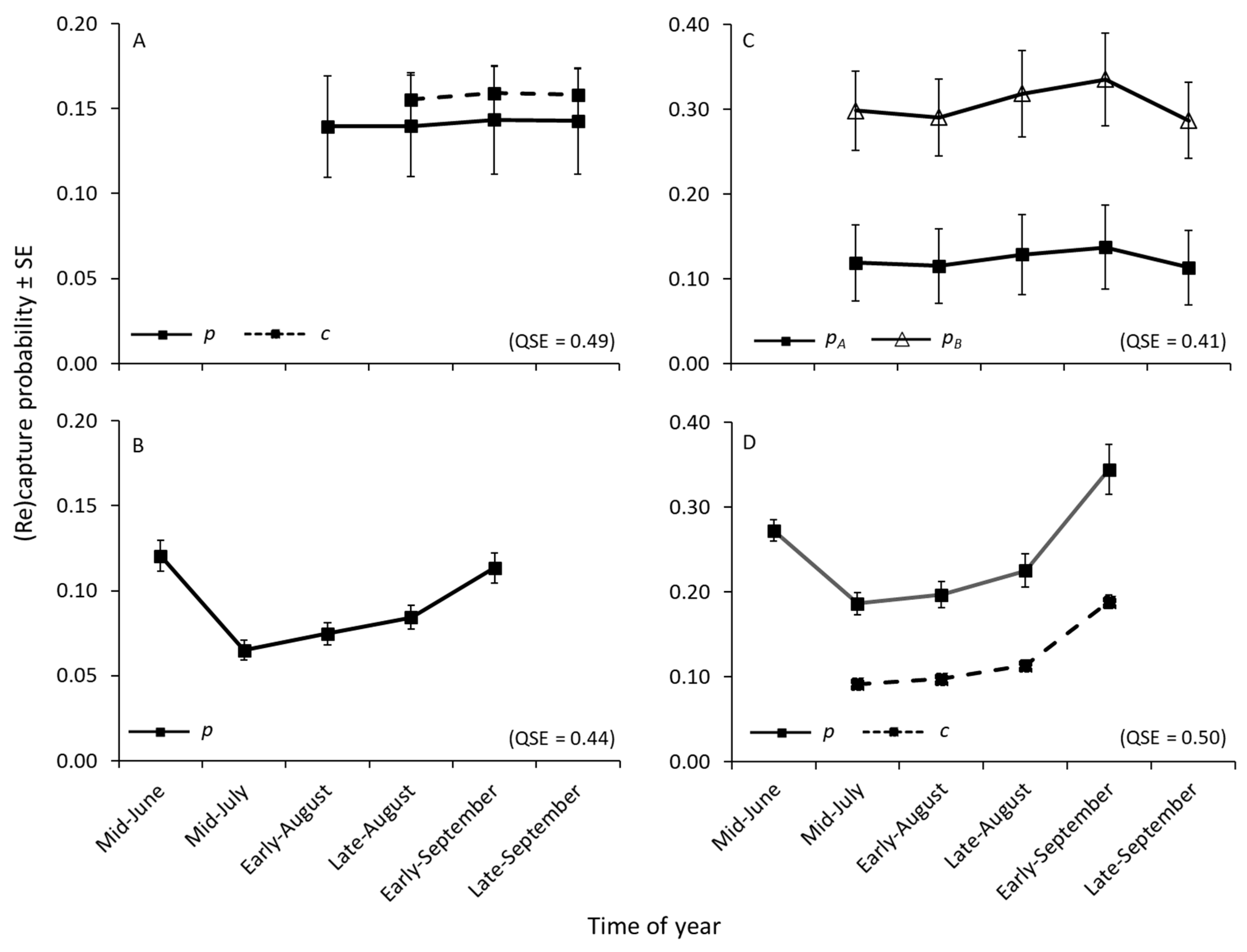
Our results were in agreement with those of previous CMR studies and indicated that capture probabilities varied among species, by time, and were associated with shell length. Although our mean capture probability estimates for E. capsaeformis (2–6%) were lower than those reported for other species during the warmer months by Villella et al. [26] (7–19%), Meador et al. [27] (8–20%), and Watson et al. [75] (10–30%), our estimated capture probabilities for A. pectorosa (10–34%) and M. conradicus (6–16%) were similar. The lower capture rates of E. capsaeformis may reflect the difficulty of detecting a species existing at much lower densities (<0.4/m2) than our other two study species, or be related to species-specific behavior or smaller shell size. Actinonaias pectorosa had the highest capture probabilities, presumably because individuals were comparatively larger in length and aperture size relative to other target species. Interestingly, intra-annual temporal trends in capture were similar across all three study species. Capture probabilities were higher in mid-June, and then declined by mid-July before steadily increasing through late September. Because all three species are long-term brooders—spawning in late summer and autumn, gravid through winter, and releasing glochidia the following late spring to early summer—capture probabilities may have reflected vertical migration patterns associated with reproductive behavior. Because species-specific mean capture probabilities were different between years, but intra-annual trends were similar among species, inter-annual variability in environmental conditions (e.g., temperature, stream discharge) additionally may have played a role.
Obtaining unbiased and precise estimates of specific-specific vital rates and identifying factors influencing mussel survival are important for developing effective conservation plans. Previous CMR studies have reported that annual mussel survival can be influenced by several factors, including age, shell length, habitat type, stream discharge, and invasive unionid densities [25,26,27,29,71]. Over a four-year CMR study, Villella et al. [26] estimated high annual apparent survival rates (>90%) for adult Elliptio complanata, E. fisheriana, and Lampsilis cariosa, and found that survival was time- and size-dependent. Using a Passive Integrated Transponder-tag CMR methodology, Hua et al. [30] documented high monthly survival rates (>98%) for Cumberlandian combshell (Epioblasma brevidens) in the Powell River, Tennessee, over a two-year period. Additionally, during a one-year Robust Design CMR study, Meador et al. [27] reported that variations in survival differed among habitat types and were positively associated with shell length. Similar to these other CMR study findings of high adult annual survival rates (>90%), our results indicated that E. capsaeformis exhibited high annual apparent survival probabilities (>96%). By understanding the factors affecting survival, reintroduction plan details (e.g., release site habitat characteristics; age, size, sex ratios of released individuals) can be identified and recommended to optimize survival of released individuals, and ultimately, long-term restoration success.
In addition to providing important insights into the ecological relationships affecting vital rates and capture probabilities, CMR can provide invaluable data on age and growth for improving predicted length-at-age growth models, assessing age-class distributions, evaluating spatial and temporal variations in growth, predicting chance of species recovery, and estimating species risk of extinction [26,71,76,77]. Furthermore, mark-recapture studies can be used to validate previous conclusions on vital rates estimated through other approaches to assessing population parameters, such as quantitative quadrats sampling, length-at-age catch-curves or shell thin-sectioning age and growth analyses. By following unique individuals through time, we were able to estimate survival rates based on fates of individuals captured. Although original aging of uniquely marked TAs was estimated using predicted length-at-age growth curves, our study was able to assess post-release survival by integrating 2011–2012 capture histories with 2006–2011 reintroduction data (i.e., known time since release). Similarly, tagged LPSAs were of known age at release and provided concrete age-specific data for estimating annual survival rates. The results of our study were in agreement with previous predictions—high annual survival for subadult and adult age-classes—estimated using shell thin-sectioning analyses and modeling of length-at-age data of mussels collected from systematic quadrat surveys in the Clinch River, Tennessee [2].
When combined, length-at-release reintroduction data and measurements taken during the 2011–2012 study period provided a considerable amount of data on absolute growth for E. capsaeformis. However, a von Bertalanffy growth curve [78] could not accurately be fitted to our presently available growth data for several reasons: (1) the ages of TAs were extrapolated estimates based on predicted length-at-age growth curves in Jones and Neves [6], (2) LPSA growth data only represented younger age-classes (≤3 years-old), and (3) shell thin-sectioning was not conducted. Even though LPSA data provided known—as opposed to estimated— length-at-age, using the available data for 1–3-year-olds likely would have resulted in biased estimates of growth parameters. Through shell thin-sectioning and future monitoring at our study site, a complete age and growth data set for reintroduced E. capsaeformis can be compiled and a predicted length-at-age growth curve can be computed to compare to that of Jones and Neves [6]. Consequently, further data from marked individuals can be used to assess the accuracy and precision of shell thin-sectioning, test the assumptions of shell annuli formation for E. capsaeformis, and examine disturbance ring deposition for reintroduced individuals [79,80].
Also of concern is whether sampling and monitoring efforts can cause declines in abundance and density due to disturbance. Mussels are known to lay down disturbance rings, which represent brief cessations of growth due to factors such as handling or natural disturbances, but it is unknown how much disturbance—through the excavation of substrate or removal of mussels from substrate for processing—influences mortality rates or increases displacement of individuals [80]. In this study, CMR estimators indicated a significant decline in A. pectorosa abundance between 2011 and 2012; a trend not detected by the systematic quadrat survey. It is likely that displacement from the site—rather than natural or induced mortality—was responsible for this estimated decline in abundance. Other multiyear studies suggested low to no mortality from presumed similar levels of handling stress, nor did they reveal related declines in abundance [26,80,81]. Even though all mussels were returned to the area where they were found in the substrate, the average size of A. pectorosa individuals was larger than our other study species, and these mussels may have had a more difficult time reburrowing into the substrate after handling. This, in combination with surveyors moving about on the streambed and high flow events after surveying, may have displaced some A. pectorosa individuals downstream out of the survey area, resulting in the decline in abundance noted from the effective sampling area. Further examination is needed to assess whether this decline in abundance, estimated through CMR, can be attributed to mortality (natural or handling associated) or due to displacement outside the study area.
Despite the large number of mussel population restoration projects that have been conducted over the last century [73], few have determined the long-term success of these efforts [82]. Detecting population trends, estimating species-specific vital rates, identifying factors influencing capture and survival, and long-term monitoring of population dynamics are essential to developing effective conservation plans and to determine long-term success of reintroduction efforts [5]. By performing and reporting post-restoration population monitoring, projects can provide insight into the relative success of method-specific restoration efforts and population viability. Both systematic quadrat and CMR sampling techniques have useful applications in population monitoring—and towards assessing population viability—but are dependent on project objectives.
Our results indicated that CMR has advantages over quadrat sampling for quantitatively monitoring mussel populations. Incorporating appropriate CMR methodologies into monitoring studies can provide greater insight into species-specific population dynamics through the ability to account for imperfect detection, increase sample size, and ultimately produce more reliable and precise population parameter estimates. However, CMR sampling can be considerably more resource-intensive than other probability-based designs, depending on the scope of the project and CMR study design. While our study was sampling-intensive in order to thoroughly compare CMR to systematic quadrat sampling population size estimators for mussels, there are many different—and less resource-intensive—sampling and data collection approaches, data analysis strategies, and statistical models available for biologists to consider when designing a CMR study. Developing an effective, efficient, and feasible monitoring program that can achieve desired goals requires identifying clearly defined and quantifiable objectives to guide informed survey design decisions [10,43,69].
In addition to taking project objectives and availability of resources into consideration, the selection of an appropriate sampling design for monitoring and analysis should consider other factors such as study site characteristics and species’ expected densities and distributions [8]. For example, biologists interested in employing CMR sampling across large study areas (e.g., >2000 m2), or in difficult-to-sample habitats, could consider stratifying reaches (e.g., habitat type, species’ densities, distributions) and allocating efforts to randomly chosen sampling units (e.g., line-transects) within randomly selected reaches because it would be less resource intensive and could still provide improved reliability and precision in population estimates relative to quadrat sampling [27]. Alternatively, if a study area is relatively small (e.g., <500 m2), a CMR design surveying the entire substrate surface area could easily be implemented in a cost-effective manner. Finally, a Robust Design (integrated closed- and open-population parameter estimators) CMR study is recommended for long-term (≥3 years) monitoring as it allows for estimation of abundance and true survival with improved precision, (temporary) emigration, and recruitment rates—which is crucial to evaluating population viability [2,21,26,27,31,33,83,84]. Overall, CMR approaches are appropriate and feasible for monitoring populations within or across a few study sites. However, further research is needed on the applicability and feasibility of CMR sampling to watershed-wide (i.e., spatially extensive) assessments compared to other alternative, less intensive, designs.
We recommend that monitoring projects use quadrat sampling approaches when the objective is to simply estimate and detect trends in population size for established, or restored, species of moderate to high densities (>0.2/m2). Capture-mark-recapture should be used or incorporated into existing monitoring programs when objectives include assessing restored populations of reintroduced or augmented species at low to moderate densities, obtaining reliable and precise estimates of population parameters (e.g., survival, recruitment), or producing unbiased estimates of abundance with precision for species occurring at low to moderate densities (≤0.2/m2). Future mussel restoration efforts should uniquely mark released individuals and incorporate a CMR monitoring and analysis component to the project to improve our understanding of species-specific demographic characteristics as well as to assess likelihood of population restoration success (Table 6).
Even though there was not enough data on recruited E. capsaeformis for CMR models, our observations confirmed that natural recruitment is occurring—a measure of short-term reintroduction success. We believe long-term reintroduction success could not be assessed in our 2011–2012 surveys due to the time frame of the project, i.e., monitoring immediately followed reintroductions and consequential natural recruitment can take several years before it is self-sustaining and evident. Continued long-term monitoring efforts will be essential to evaluating E. capsaeformis recruitment rates at the restoration site and determine if they are reaching self-sustaining levels or are in need of additional augmentations. Results from this follow-up monitoring study, and future monitoring efforts, will improve our understanding of E. capsaeformis vital rates, and provide data on effective population sizes and demographic structures required to make informed decisions for future recovery projects. In accordance with the recovery plan for E. capsaeformis [1], we recommend biennial CMR monitoring efforts at Cleveland Islands, Virginia to reveal whether these recovery efforts were ultimately successful at restoring a long-term viable deme of E. capsaeformis to the Upper Clinch River—information essential for effective future management and recovery plans.

Author Contributions

All authors contributed to the conceptualization, initial study design, and manuscript preparation (writing—original draft preparation C.S.C. and J.W.J.; writing—review and editing, R.S.B., E.M.H., and M.J.K.; methodology, all).; investigation, C.S.C. and J.W.J. with the assistance of R.S.B.; formal analysis, C.S.C. (with the technical guidance of M.J.K. on mark-recapture models and M.J.K. and R.S.B. with data interpretation); visualization, all; supervision, J.W.J.; funding acquisition, J.W.J. and R.S.B.

Funding

This research was funded by the U.S. Fish and Wildlife Service, Gloucester, Virginia, and Asheville, North Carolina, Field Offices.

Acknowledgments

We thank Drew Phipps, Tim Lane, Jen Rogers, Steve Ahlstedt, and the many other individuals who assisted on this large-scale monitoring project from the U.S. Fish and Wildlife Service (USFWS), the Virginia Department of Game and Inland Fisheries (VDGIF), The Nature Conservancy (TNC), Daguna Consulting, and Virginia Tech. We thank Dan Catlin at Virginia Tech for assisting C.C. with mark-recapture modeling and data analysis in Program MARK. We especially thank Dr. Braven Beaty (TNC, Abingdon, Virginia) and Mike Pinder (VDGIF, Blacksburg, Virginia) for their involvement throughout this study and for access to Cleveland Islands. The views expressed in this article are those of the authors and do not necessarily represent those of the USFWS.

Conflicts of Interest

The authors declare no conflict of interest.

Appendix A

Table A1. An example of a Program MARK input file for Epioblasma capsaeformis closed-population modeling. The first two columns represent the unique mark (tag identification) of an individual and its associated encounter history over five sampling occasions. The next three columns represent the individual’s associated group (TA = translocated adult, LPSA = laboratory-propagated subadult, or recruit; can only be associated with one group), followed by three columns for individual covariates representing mean shell length at capture and sex classification. Sex classification was coded as follows (sex1 = #, sex2 = #): 1,0 = female, 0,1 = male, and 1,1 = sex unknown.
/*IDEncounter HistoryGrp1 = TAGrp2 = LPSAGrp3 = recruitCov = lengthCov = sex1Cov = sex2Semicolon*/
/*ECAPS001*/000011002701;
/*ECAPS002*/000101002501;
/*ECAPS003*/000111002410;
/*ECAPS004*/001001002010;
/*ECAPS005*/001010103510;
/*ECAPS006*/001100104010;
/*ECAPS007*/001110104201;
/*ECAPS008*/010000103201;
/*ECAPS009*/010010102901;
/*ECAPS010*/111100011511;
.........
.........
.........
.........
/*ECAPS999*/111110012011;
Table A2. An example of a Program MARK input file for Actinonaias pectorosa closed-population modeling. The first two columns represent the unique mark (tag identification) of an individual and its associated encounter history over five sampling occasions. The next column represents encounter history frequency (1s when modeling individual encounter histories), followed by a column for an individual covariate (mean shell length at capture within study period). The input files for Medionidus conradicus followed the same formatting, with the exception of the 2011 encounter histories that consisted of only four sampling occasions.
/*IDEncounter HistoryFrequencyCov = LengthSemicolon*/
/*APECT001*/100111111;
/*APECT002*/10100185;
/*APECT003*/10101190;
/*APECT004*/10110165;
/*APECT005*/10111140;
/*APECT006*/11000199;
/*APECT007*/11001164;
/*APECT008*/11010188;
/*APECT009*/110111101;
/*APECT010*/111011109;
.....
.....
.....
.....
/*APECT999*/110111105;
Table A3. Species collected at Cleveland Islands (furthest left-descending channel) in the Upper Clinch River, Russel County, Virginia, using systematic quadrat (with multiple random starts) and capture-mark-recapture (CMR) sampling approaches in 2011 and 2012.
20112012
SpeciesCommon NameQuadratsCMRQuadratsCMR
Actinonaias ligamentinaMucket XXX
Actinonaias pectorosaPheasantshellXXXX
Amblema plicataThreeridge X
Cyclonaias tuberculataPurple wartybackXX X
Elliptio crassidensElephantear X
Elliptio dilatataSpikeXXXX
Epioblasma brevidensFECumberlandian combshellXXXX
Epioblasma capsaeformisFEOyster musselXXXX
Epioblasma triquetraFESnuffbox XXX
Fusconaia corFEShiny pigtoeXXXX
Fusconaia cuneolusFEFine-rayed pigtoeXXXX
Fusconaia subrotundaLongsolidXXXX
Lampsilis fasciolaWavy-rayed lampmusselXXXX
Lampsilis ovataPocketbookXXXX
Lasmigona costataFlutedshellXXXX
Ligumia rectaBlack sandshell X X
Medionidus conradicusCumberland moccasinshellXXXX
Plethobasus cyphyusFESheepnose X X
Pleurobema oviformeTennessee clubshellXXXX
Pleuronaia barnesianaTennessee pigtoeXXXX
Pleuronaia dolabelloidesFESlabside pearlymusselXX X
Ptychobranchus fasciolarisKidneyshellXXXX
Ptychobranchus subtentusFEFluted kidneyshellXX X
Quadrula cylindrica strigillataFERough rabbitsfootXX X
Villosa irisRainbowXXXX
Villosa vanuxemensisMountain creekshellXXXX
Figure A1. Cormack–Jolly–Seber (CJS) open-capture model diagram for Epioblasma capsaeformis at Cleveland Islands in the Upper Clinch River, Russel County, Virginia from reintroductions and capture-mark-recapture (CMR) sampling in 2006–2012. Black numbered boxes = encounter history occasions, blue capture parameters ( p i ) = recapture probability during encounter occasions, and red survival parameters ( φ i ) = apparent survival probability between successive encounter occasions. Boxes 1–5 represent 2006–2010 annual releases of E. capsaeformis (parameters p 2 p 5 fixed at 0), box 11 represents a 2011 release event (parameter p 11 fixed at 0) that occurred between the 2011–2012 CMR sampling study periods, and boxes 6–10 and 12–16 represent active CMR sampling conducted over five encounter occasions within each study period (2011–2012; p 6 p 10 and p 12 p 16 parameters time-dependent). Survival parameters within the 2011 and 2012 closed-capture study periods ( φ 6 φ 9 , φ 11 φ 15 ) were fixed at 1.
Diversity 11 00127 g0a1

References

  1. U.S. Fish and Wildlife Service. Recovery Plan for Cumberland Elktoe (Alasmidonta atropurpurea), Oyster Mussel (Epioblasma capsaeformis), Cumberlandian Combshell (Epioblasma brevidens), Purple Bean (Villosa perpurpurea), and Rough Rabbitsfoot (Quadrula cylindrica strigillata); U.S. Fish and Wildlife Service, Asheville Field Office: Asheville, NC, USA, 2004; p. 167.
  2. Jones, J.W.; Neves, R.J.; Hallerman, E.M. Population Performance Criteria to Evaluate Reintroduction and Recovery of Two Endangered Mussel Species, Epioblasma brevidens and Epioblasma capsaeformis (Bivalvia: Unionidae). Freshw. Mollusk Biol. Conserv. 2012, 15, 27–45. [Google Scholar] [CrossRef] [Green Version]
  3. Carey, C.S.; Jones, J.W.; Butler, R.S.; Hallerman, E.M. Restoring the endangered oyster mussel (Epioblasma capsaeformis) to the upper Clinch River, Virginia: An evaluation of population restoration techniques. Restor. Ecol. 2015, 23, 447–454. [Google Scholar] [CrossRef]
  4. Sarrazin, F.; Barbault, R. Reintroduction: Challenges and lessons for basic ecology. Trends Ecol. Evol. 1996, 11, 474–478. [Google Scholar] [CrossRef]
  5. Sarrazin, F.; Legendre, S. Demographic Approach to Releasing Adults versus Young in Reintroductions. Conserv. Biol. 2000, 14, 488–500. [Google Scholar] [CrossRef]
  6. Jones, J.W.; Neves, R.J. Influence of life-history variation on demographic responses of three freshwater mussel species (Bivalvia: Unionidae) in the Clinch River, USA. Aquat. Conserv. Mar. Freshw. Ecosyst. 2011, 21, 57–73. [Google Scholar] [CrossRef]
  7. Christman, M.C. A Review of Quadrat-Based Sampling of Rare, Geographically Clustered Populations. J. Agric. Biol. Environ. Stat. 2000, 5, 168. [Google Scholar] [CrossRef]
  8. Pooler, P.S.; Smith, D.R. Optimal sampling design for estimating spatial distribution and abundance of a freshwater mussel population. J. N. Am. Benthol. Soc. 2005, 24, 525–537. [Google Scholar] [CrossRef]
  9. Thompson, S.K. Sampling, 3rd ed.; John Wiley & Sons. Inc.: Hoboken, NJ, USA, 2012; ISBN 978-0-470-40231-3. [Google Scholar]
  10. Strayer, D.L.; Smith, D.R. A Guide to Sampling Freshwater Mussel Populations; American Fisheries Society: Bethesda, MD, USA, 2003. [Google Scholar]
  11. Miranda, L.E.; Bettoli, P.W. Analysis and Interpretation of Freshwater Fisheries Data; Guy, C.S., Brown, M.L., Eds.; American Fisheries Society: Bethesda, MD, USA, 2007; pp. 229–277. [Google Scholar]
  12. Petersen, C.G.J. The yearly immigration of young plaice into the Limfjord from the German Sea. Rep. Dan. Biol. Stn. 1895, 6, 1–77. [Google Scholar]
  13. Lincoln, F.C. Calculating Waterfowl Abundance on the Basis of Banding Returns; U.S. Department of Agriculture, Biological Survey Bureau: Falls Church, VA, USA, 1930; pp. 1–4.
  14. Young, H.; Neess, J.; Emlen, J.T. Heterogeneity of Trap Response in a Population of House Mice. J. Wildl. Manag. 1952, 16, 169. [Google Scholar] [CrossRef]
  15. Seber, G.A.F. The multi-sample single recapture census. Biometrika 1962, 49, 339–350. [Google Scholar] [CrossRef]
  16. Jolly, G.M. Estimates of population parameters from multiple recapture data with both death and dilution—Deterministic model. Biometrika 1963, 50, 113–128. [Google Scholar]
  17. Jolly, G.M. Explicit Estimates from Capture-Recapture Data with Both Death and Immigration-Stochastic Model. Biometrika 1965, 52, 225. [Google Scholar] [CrossRef] [PubMed]
  18. Cormack, R.M. Estimates of Survival from the Sighting of Marked Animals. Biometrika 1964, 51, 429. [Google Scholar] [CrossRef]
  19. Edwards, W.R.; Eberhardt, L.L. Estimating cottontail abundance from live-trapping data. J. Wild. Manag. 1967, 31, 87–96. [Google Scholar] [CrossRef]
  20. Otis, D.L.; Burnham, K.P.; White, G.C.; Anderson, D.R. Statistical inference from capture data on closed animal population. Wild. Mono 1978, 62, 3–135. [Google Scholar]
  21. Pollock, K.H.; Nichols, J.D.; Brownie, C.; Hines, J.E. Statistical inference for capture-recapture experiments. Wildl. Monogr. 1990, 107, 3–97. [Google Scholar]
  22. Mowat, G.; Strobeck, C. Estimating Population Size of Grizzly Bears Using Hair Capture, DNA Profiling, and Mark-Recapture Analysis. J. Wildl. Manag. 2000, 64, 183. [Google Scholar] [CrossRef]
  23. Albanese, B.; Angermeier, P.L.; Dorai-Raj, S. Ecological correlates of fish movement in a network of Virginia streams. Can. J. Fish. Aquat. Sci. 2004, 61, 857–869. [Google Scholar] [CrossRef]
  24. Silver, S.C.; Ostro, L.E.T.; Marsh, L.K.; Maffei, L.; Noss, A.J.; Kelly, M.J.; Wallace, R.B.; Gómez, H.; Ayala, G. The use of camera traps for estimating jaguar Panthera onca abundance and density using capture/recapture analysis. Oryx 2004, 38, 148–154. [Google Scholar] [CrossRef]
  25. Hart, R.A.; Grier, J.W.; Miller, A.C.; Davis, M. Empirically Derived Survival Rates of a Native Mussel, Amblema plicata, in the Mississippi and Otter Tail Rivers, Minnesota. Am. Midl. Nat. 2001, 146, 254–263. [Google Scholar] [CrossRef]
  26. Villella, R.F.; Smith, D.R.; Lemarié, D.P. Estimating Survival and Recruitment in a Freshwater Mussel Population Using Mark-recapture Techniques. Am. Midl. Nat. 2004, 151, 114–133. [Google Scholar] [CrossRef]
  27. Meador, J.R.; Peterson, J.T.; Wisniewski, J.M. An evaluation of the factors influencing freshwater mussel capture probability, survival, and temporary emigration in a large lowland river. J. N. Am. Benthol. Soc. 2011, 30, 507–521. [Google Scholar] [CrossRef]
  28. Carey, C.S. An Evaluation of Population Restoration and Monitoring Techniques for Freshwater Mussels in the Upper Clinch River, Virginia, and Refinement of Culture Methods for Laboratory-Propagated juveniles. Master’s Thesis, Virginia Polytechnic Institute and State University, Blacksburg, VA, USA, 2013. [Google Scholar]
  29. Wisniewski, J.M.; Shea, C.P.; Abbott, S.; Stringfellow, R.C. Imperfect Recapture: A Potential Source of Bias in Freshwater Mussel Studies. Am. Midl. Nat. 2013, 170, 229–247. [Google Scholar] [CrossRef]
  30. Hua, D.; Jiao, Y.; Neves, R.J.; Jones, J.W. Using PIT tags to assess individual heterogeneity in a mark-recapture study of laboratory-reared juveniles of the endangered Cumberlandian combshell (Epioblasma brevidens). Ecol. Evol. 2015, 5, 1076–1087. [Google Scholar] [CrossRef] [PubMed]
  31. Wisniewski, J.M.; Abbott, S.; Gascho Landis, A.M. An evaluation of streamflow augmentation as a short-term freshwater mussel conservation strategy. River Res. App. 2016, 32, 1166–1178. [Google Scholar] [CrossRef]
  32. Seber, G.A.F. The Estimation of Animal Abundance and Related Parameters, 2nd ed.; MacMillian Publishing: New York, NY, USA, 1982. [Google Scholar]
  33. Pollock, K.H. A Capture-Recapture Design Robust to Unequal Probability of Capture. J. Wildl. Manag. 1982, 46, 752. [Google Scholar] [CrossRef]
  34. Lebreton, J.-D.; Burnham, K.P.; Clobert, J.; Anderson, D.R. Modeling Survival and Testing Biological Hypotheses Using Marked Animals: A Unified Approach with Case Studies. Ecol. Monogr. 1992, 62, 67–118. [Google Scholar] [CrossRef] [Green Version]
  35. Kendall, W.L.; Nichols, J.D.; Hines, J.E. Estimating temporary emigration using capture-recapture data with Polluck’s robust design. Ecology 1997, 78, 563–578. [Google Scholar]
  36. Pollock, K.H. A K—Sample tag-recapture model allowing for unequal survival and catchability. Biometrika 1975, 62, 577–583. [Google Scholar] [CrossRef]
  37. Pollock, K.H. Capture-Recapture Models Allowing for Age-Dependent Survival and Capture Rates. Biometrika 1981, 37, 521. [Google Scholar] [CrossRef]
  38. Pollock, K.H.; Otto, M.C. Robust Estimation of Population Size in Closed Animal Populations from Capture-Recapture Experiments. Biometrika 1983, 39, 1035. [Google Scholar] [CrossRef] [Green Version]
  39. White, G.C.; Anderson, D.R.; Burnham, K.P.; Otis, D.L. Capture-Recapture and Removal Methods for Sampling Closed Populations; Los Alamos National Laboratory: Los Alamos, NM, USA, 1982. [Google Scholar]
  40. Hornbach, D.J.; Deneka, T. A Comparison of a Qualitative and a Quantitative Collection Method for Examining Freshwater Mussel Assemblages. J. N. Am. Benthol. Soc. 1996, 15, 587–596. [Google Scholar] [CrossRef]
  41. Smith, D.R.; Villella, R.F.; Lemarié, D.P.; von Oettingen, S. How much excavation is needed to monitor freshwater mussels? In Freshwater Mollusk Symposia Proceedings; Ohio Biological Survey: Columbus, OH, USA, 2000; pp. 203–218. [Google Scholar]
  42. Macnaughton, C.J.; Harvey-Lavoie, S.; Senay, C.; Lanthier, G.; Bourque, G.; Legengre, P.; Boisclair, D. A comparison of electrofishing and visual surveying methods for estimating fish community structure in temperate rivers. River Res. Appl. 2015, 31, 1040–1051. [Google Scholar] [CrossRef]
  43. Gitzen, R.A.; Millspaugh, J.J.; Copper, A.B.; Licht, D.S. Design and Analysis of Long-term Ecological Monitoring Studies; Cambridge University Press: New York, NY, USA, 2012. [Google Scholar]
  44. Eckert, N.L.; Pinder, M.J. Freshwater Mussel Survey of Cleveland Island, Clinch River, Virginia: Augmentation Monitoring Site 2008; Virginia Department of Game and Inland Fisheries: Richmond, VA, USA, 2010.
  45. Virginia Department of Game and Inland Fisheries. Virginia Freshwater Mussel Restoration Strategy: Upper Tennessee River Basin. Bureau of Wildlife Resources; Wildlife Diversity Division, Nongame and Endangered Wildlife Program: Richmond, VA, USA, 2010.
  46. Jones, J.W.; Ahlstedt, S.A.; Ostby, B.J.K.; Beaty, B.; Pinder, M.; Eckert, N.; Butler, R.S.; Hubbs, D.; Walker, C.; Hanlon, S.; et al. Clinch River Freshwater Mussels Upstream of Norris Reservoir, Tennessee and Virginia: A Quantitative Assessment from 2004–2014. J. Am. Water Resour. Assoc. 2014, 50, 820–836. [Google Scholar] [CrossRef]
  47. Price, J.E.; Zipper, C.E.; Jones, J.W.; Frank, C.W. Water and Sediment Quality in the Clinch River of Virginia and Tennessee, 1964–2010. J. Am. Water Resour. Assoc. 2014, 50, 837–858. [Google Scholar] [CrossRef]
  48. Jones, J.W. A Holistic Approach to Taxonomic Evaluation of Two Closely Related Endangered Freshwater Mussel Species, the Oyster Mussel (Epioblasma capsaeformis) and tan riffleshell (Epioblasma florentina walkeri) (Bivalvia: Unionidae). Master’s Thesis, Virginia Polytechnic Institute and State University, Blacksburg, VA, USA, 2004. [Google Scholar]
  49. Jones, J.W.; Hallerman, E.M.; Neves, R.J. Genetic management guidelines for captive propagation of freshwater mussels (unionoidea). J. Shellfish. Res. 2006, 25, 527–535. [Google Scholar] [CrossRef]
  50. Smith, D.R.; Villella, R.F.; Lemarié, D.P. Survey protocol for assessment of endangered freshwater mussels in the Alleghany River, Pennsylvania. J. N. Am. Benth. Soc. 2001, 20, 118–132. [Google Scholar] [CrossRef]
  51. White, G.C.; Burnham, K.P. Program MARK: survival estimation from populations of marked animals. Bird Study 1999, 46, S120–S139. [Google Scholar] [CrossRef]
  52. White, G.C. Closed population estimation models and their extensions in Program MARK. Environ. Ecol. Stat. 2008, 15, 89–99. [Google Scholar] [CrossRef]
  53. Huggins, R.M. On the Statistical Analysis of Capture Experiments. Biometrika 1989, 76, 133–140. [Google Scholar] [CrossRef]
  54. Huggins, R.M. Some Practical Aspects of a Conditional Likelihood Approach to Capture Experiments. Biometrika 1991, 47, 725. [Google Scholar] [CrossRef]
  55. Chao, A. Estimating the Population Size for Capture-Recapture Data with Unequal Catchability. Biometrika 1987, 43, 783. [Google Scholar] [CrossRef]
  56. Chao, A. Estimating Population Size for Sparse Data in Capture-Recapture Experiments. Biometrika 1989, 45, 427. [Google Scholar] [CrossRef]
  57. Williams, B.K.; Nichols, J.D.; Conroy, M.J. Analysis and Management of Animal Populations: Modeling, Estimation, and Decision Making; Academic Press: New York, NY, USA, 2002. [Google Scholar]
  58. Pledger, S.; Pollock, K.H.; Norris, J.L. Open capture-recapture models with heterogeneity: I. Cormark-Jolly-Seber model. Biometrics 2003, 59, 786–794. [Google Scholar] [CrossRef] [PubMed]
  59. Stanley, T.R.; Burnham, K.P. A closure test for time-specific capture-recapture data. Environ. Ecol. Stat. 1999, 6, 197–209. [Google Scholar] [CrossRef]
  60. Burnham, K.P.; Anderson, D.R. Model Selection and Inference: A Practical Information-Theoretical Approach; Springer: New York, NY, USA, 1998. [Google Scholar]
  61. White, G.C.; Burnham, K.P.; Anderson, D.R. Advanced Features of Program Mark. In Integrating People and Wildlife for a Sustainable Future, In Proceedings of the Second International Wildlife Management Congress, Bethesda, MD, USA; Field, R., Warren, R.J., Okarma, H., Sievert, P.R., Eds.; The Wildlife Society: Bethesda, MD, USA, 2001; pp. 368–377. [Google Scholar]
  62. Boulanger, J.; White, G.C.; McLellan, B.N.; Woods, J.; Proctor, M.; Himmer, S. A meta-analysis of grizzly bear DNA mark-recapture projects in British Columbia, Canada. Ursus 2002, 13, 137–152. [Google Scholar]
  63. Hua, D.; Rogers, J.; Jones, J.; Neves, R. Propagation, Culture, and Monitoring of Endangered Mussels for Population Restoration in the Clinch and Powell Rivers, Tennessee, 2006–2010; Tennessee Wildlife Resources Agency: Nashville, TN, USA, 2011. [Google Scholar]
  64. Anderson, D.R.; Burnham, K.P.; Thompson, W.L. Null Hypothesis Testing: Problems, Prevalence, and an Alternative. J. Wildl. Manag. 2000, 64, 912. [Google Scholar] [CrossRef]
  65. Johnson, J.B.; Omland, K.S. Model selection in ecology and evolution. Trends Ecol. Evol. 2004, 19, 101–108. [Google Scholar] [CrossRef]
  66. Dennis, S.D. Distributional Analysis of the Freshwater Mussel Fauna of the Tennessee River System, with Special Reference to Possible Limiting Effects of Siltation, Report No. 85-2; Tennessee Wildlife Resources Agency: Nashville, TN, USA, 1985. [Google Scholar]
  67. Ahlstedt, S.A.; Fagg, M.T.; Butler, R.S.; Connell, J.F.; Jones, J.W. Quantitative monitoring of freshwater mussel populations from 1979-2004 in the Clinch and Powell Rivers of Tennessee and Virginia, and an historical perspective on the conservation status of the fauna. J. Moll. Biol. Conserv. 2016, 19, 1–18. [Google Scholar]
  68. Green, R.H.; Young, R.C. Sampling to detect rare species. Ecol. App. 1993, 3, 351–356. [Google Scholar] [CrossRef]
  69. Smith, D.R. Survey design for detecting rare freshwater mussels. J. N. Am. Benthol. Soc. 2006, 25, 701–711. [Google Scholar] [CrossRef]
  70. Amyot, J.-P.; Downing, J.A. Endo- and Epibenthic Distribution of the Unionid Mollusc Elliptio complanata. J. N. Am. Benthol. Soc. 1991, 10, 280–285. [Google Scholar] [CrossRef]
  71. Inoue, K.; Levine, T.D.; Lang, B.K.; Berg, D.J. Long-term mark-and-recapture study of a freshwater mussel reveals patterns of habitat use and an association between survival and river discharge. Freshw. Biol. 2014, 59, 1872–1883. [Google Scholar] [CrossRef]
  72. Watters, G.T.; O’Dee, S.H.; Chordas, S., III. Patterns of vertical migration in freshwater mussels (Bivalvia: Unionida). J. Fresh. Ecol. 2001, 16, 541–549. [Google Scholar] [CrossRef]
  73. Haag, W.R. North American Freshwater Mussels: Natural History, Ecology, Conservation; Cambridge University Press: Cambridge, UK, 2012. [Google Scholar]
  74. Balfour, D.L.; Smock, L.A. Distribution, Age Structure, and Movements of the Freshwater Mussel Elliptio complanata (Mollusca: Unionidae) in a Headwater Stream. J. Freshw. Ecol. 1995, 10, 255–268. [Google Scholar] [CrossRef]
  75. Watson, B.; Ostby, B.; Carey, C. Using Mark-Recapture to Assess Populations of the Endangered James Spinymussel (Pleurobema Collina). In Proceedings of the 8th Biennial Freshwater Mollusk Conservation Society Symposium, Guntersville, AL, USA, 10–14 March 2013. [Google Scholar]
  76. Dennis, B.; Munholland, P.L.; Scott, J.M. Estimation of Growth and Extinction Parameters for Endangered Species. Ecol. Monogr. 1991, 61, 115–143. [Google Scholar] [CrossRef]
  77. Haag, W.R.; Rypel, A.L. Growth and longevity in freshwater mussels: Evolutionary and conservation implications. Biol. Rev. 2011, 86, 225–247. [Google Scholar] [CrossRef] [PubMed]
  78. Von Bertalanffy, L. A quantitative theory of organic growth. Hum. Biol. 1938, 10, 181–213. [Google Scholar]
  79. Dycus, J.C.; Wisniewski, J.M.; Peterson, J.T. The effects of flow and stream characteristics on the variation in freshwater mussel growth in a Southeast US river basin. Fresh. Biol. 2015, 60, 395–409. [Google Scholar] [CrossRef]
  80. Haag, W.R.; Commens-Carson, A.M. Testing the assumption of annual shell ring deposition in freshwater mussels. Can. J. Fish. Aquat. Sci. 2008, 65, 493–508. [Google Scholar] [CrossRef]
  81. Kesler, D.H.; Downing, J.A. Internal shell annuli yield inaccurate growth estimates in freshwater mussels Elliptio complanata and Lampsilis radiata. Fresh. Biol. 1997, 37, 325–332. [Google Scholar] [CrossRef]
  82. Cope, W.G.; Waller, D.L. Evaluation of freshwater mussel relocation as a conservation and management strategy. Regul. Rivers Res. Manag. 1995, 11, 147–155. [Google Scholar] [CrossRef]
  83. Lettink, M.; Armstrong, D.P. An Introduction to Using Mark-Recapture Analysis for Monitoring Threatened Species. In Department of Conservation Technical Series A; Publishing Team, New Zealand Department of Conservation: Wellington, New Zealand, 2003; Volume 28, pp. 5–32. [Google Scholar]
  84. Kendall, W.L. The robust design for capture-recapture studies: Analysis using program MARK. In Integrating People and Wildlife for a Sustainable Future, Proceedings of the Second International Wildlife Management Congress, Godollo, Hungary, June 28–July 2 1999; Field, R., Warren, R.J., Okarma, H., Sievert, P.R., Eds.; The Wildlife Society: Bethesda, MD, USA, 2001; pp. 357–360. [Google Scholar]
Figure 1. Capture (p) probabilities (±SE) for 2011 (A) and 2012 (B) translocated adult and released laboratory-propagated subadult Epioblasma capsaeformis by CMR sampling occasion at Cleveland Islands, Upper Clinch River, Russel County, Virginia estimated using closed-capture models in Program MARK. Raw estimates of quadrat sampling efficiency (QSE) on the substrate surface in late September are shown for comparison.
Diversity 11 00127 g001
Figure 2. Capture (p) and recapture (c) probabilities (±SE) for native Medionidus conradicus (A = 2011, B = 2012) and Actinonaias pectorosa (C = 2011, D = 2012) by CMR sampling occasion at Cleveland Islands, Upper Clinch River, Russel County, Virginia estimated using closed-capture models in Program MARK. Best approximating models for A. pectorosa in 2011 (C) indicated heterogeneity in capture probabilities (π = 0.59 = probability an individual belongs to mixture A), where p A = capture probabilities for mixture A and p B = capture probabilities for mixture B. Raw estimates of quadrat sampling efficiency (QSE) on the substrate surface in late September are shown for comparison.
Diversity 11 00127 g002
Table 1. Definitions for real and derived parameters, and variables used in 2011 and 2012 Epioblasma capsaeformis, Actinonaias pectorosa, and Medionidus conradicus Huggins Closed-Capture models (and E. capsaeformis Cormack–Jolly–Seber models) in Program MARK.
Parameter/Variable NotationDescription
Real parameters
p()Probability of initial capture
c()Probability of recapture
pi()Finite mixture parameter to account for effects of individual heterogeneity. The proportion of the population that belongs to mixture 1 of 2.
φ()Apparent survival probability between years
Derived parameters
  N ^   Abundance estimate
Variables
.Constant (re)capture probabilities
TTemporal variation
GGroup effects
HHeterogeneity effects
p (), c () Behavior effects (recapture probabilities differ from initial capture probabilities)
p () = c () No behavior effects in capture-recapture probabilities
LengthCapture probabilities vary as a function of shell length (covariate)
SexVariability in estimates as a function of sex (covariate)
DischargeDetection varies as a function of stream discharge (a constraint of mean daily discharge imposed on capture parameters)
Table 2. Summary of systematic random quadrat and capture-mark-recapture (CMR) sampling efforts in 2011 and 2012 at Cleveland Islands in the Upper Clinch River, Russel County, Virginia. Epioblasma capsaeformis: TAs = translocated adults, LPSAs = laboratory-propagated subadults.
DescriptionSystematic Random SamplingCapture-Mark-Recapture
2011201220112012
No. systematic samples/sampling occasions4455
Total no. quadrat sampling units388347
Effort (person-hours)3943200125
Species richness (observed) 120182525
Total no. individuals encountered 244038092055536
No. unique individuals encountered (total no. CMR captures)
Epioblasma capsaeformis
TAs1111144 (179)98 (116)
LPSAs3229110 (114)132 (138)
Recruits111 (1)
All4441255 (294)230 (254)
Actinonaias pectorosa1761363771 (6141)2471 (3401)
Medionidus conradicus84881368 (1768)1088 (1309)
Quadrat sampling efficiency (QSE) 3
Epioblasma capsaeformis
TAs0.270.181.001.00
LPSAs0.130.211.001.00
Recruits0.000.001.00
All0.160.201.001.00
Actinonaias pectorosa0.410.501.001.00
Medionidus conradicus0.490.441.001.00
1 = Species list provided in Appendix A (Table A3); 2 = Includes our three study species and all nonstudy species; nonstudy species were collected only during the 1st CMR sampling occasion within each study year. 3 = Proportion (%) sampled at substrate surface.
Table 3. Abundance estimates for Epioblasma capsaeformis (TAs = translocated adults, LPSAs = laboratory-propagated subadults), Actinonaias pectorosa, and Medionidus conradicus at Cleveland Islands in the Upper Clinch River, Russel County, Virginia from systematic random quadrat and capture-mark-recapture sampling in 2011 and 2012.
Systematic Random SamplingCapture-Mark-Recapture
Study SpeciesStudy Period   N ^   SE95% CI   N ^   SE95% CI
Epioblasma capsaeformis
TAs2011580155[106, 3170]513154[312, 955]
2012656113[218, 1969]31180[203, 531]
LPSAs2011167945[1414, 1993]18851062[710, 5360]
20121719244[698, 4236]1410611[657, 3242]
Recruits20115326[2, 1238]
20126130[3, 1420]
All20112312139[1578, 3386]23981169[1043, 6080]
20122435332[1024, 5792]1721635[900, 3547]
Actinonaias pectorosa
20119210286[7558, 11224]6615492[5803, 7752]
20127929414[5687, 11056]3494150[3239, 3833]
Medionidus conradicus
20114417223[3205, 6087]3281773[2261, 5467]
20125141332[3407, 7758]2853161[2565, 3197]
Table 4. Summary of initial captures and recaptures within the 2011 and 2012 capture-mark-recapture study periods at Cleveland Islands in the Upper Clinch River, Russel County, Virginia. i = sampling occasion, j = recapture occasion, R(i) = number of unique individuals captured and released on sampling occasion i, mij = number of marked individuals released during the ith sampling occasion that were recaptured in the jth sample.
Epioblasma Capsaeformis (Translocated Adults)
mij mij
2011iR(i)j = 2345Σ mij2012iR(i)j = 2345Σ mij
Mid-July12232218Mid-June12712115
Early-August239 88016Mid-July214 1405
Late-August335 213Early-August319 437
Early-Sept449 88Late-August423 11
Late-Sept534 0Early-Sept533 0
Epioblasma Capsaeformis (Laboratory-Propagated Subadults)
mij mij
2011iR(i)j = 2345Σ mij2012iR(i)j = 2345Σ mij
Mid-July11200011Mid-June12801012
Early-August219 0000Mid-July210 0000
Late-August322 022Early-August320 123
Early-Sept422 11Late-August430 11
Late-Sept539 0Early-Sept550 0
Actinonaias Pectorosa
mij mij
2011iR(i)j = 2345Σ mij2012iR(i)j = 2345Σ mij
Mid-July1119230622115987773Mid-June19151298870112399
Early-August21155 34221487643Mid-July2534 707166207
Late-August31288 388194582Early-August3526 8485169
Early-Sept41368 371371Late-August4564 126126
Late-Sept51137 0Early-Sept5833 0
Medionidus Conradicus
mij mij
2011iR(i)j = 2345Σ mij2012iR(i)j = 2345Σ mij
Mid-July1Mid-June13432023213094
Early-August2402 676831166Mid-July2185 12161947
Late-August3409 7453127Early-August3213 271744
Early-Sept4479 9494Late-August4240 3131
Late-Sept5465 0Early-Sept5323 0
Table 5. Summary statistics for supported (ΔQAICc < 7) candidate models and top competing (ΔQAICc < 2) models used to describe (top model or ΔQAICc < 2 in model averaging) 2011 and 2012 Epioblasma capsaeformis, Actinonaias pectorosa, and Medionidus conradicus data in Program MARK. Quasi-likelihood adjusted Akaike Information Criterion differences (ΔQAICc), AIC weights (wi), model likelihood, and number of estimable parameters (K) are listed for each approximating model.
AnalysisSpeciesYearTop Approximating ModelsΔQAICcwiModel LikelihoodK
Huggins Closed-Capture
Epioblasma capsaeformis (2 frequency groups)
2011p(t*sex) = c(t*sex) + length0.001.001.005
p(t) = c(t) + length + sex16.470.000.005
2012p(t*sex) = c(t*sex) + length0.000.991.005
p(t) = c(t) + length + sex10.490.010.015
Actinonaias pectorosa
2011pi(.) p(t*h) = c(t*h) + length0.000.881.0011
pi(.) p(h), c(h) + length5.000.070.085
pi(.) p(h) = c(h) + length6.080.040.053
2012p(t), c(t) + length0.001.001.009
Medionidus conradicus
2011p(.) = c(.) + length 0.000.501.001
p(.), c(.) + length 0.690.350.712
p(t) = c(t) + length2.460.150.294
2012p(t) = c(t) + length0.000.871.005
p(t) = c(t)3.750.130.155
Huggins Closed-Capture
Epioblasma capsaeformis (1 frequency group)
2011p(t*sex) = c(t*sex) + length0.000.991.005
p(t) = c(t) + length + sex10.49<0.01<0.015
2012p(t*sex) = c(t*sex) + length0.000.991.005
p(t) = c(t) + length + sex15.06<0.01<0.015
Cormack–Jolly–Seber (16 encounter occasions)
Epioblasma capsaeformis
2006–2012φ(.) p(g + t + length)0.001.001.005
Cormack–Jolly–Seber (10 encounter occasions)
Epioblasma capsaeformis
2011–2012φ(.) p(g + length)0.001.001.005
Table 6. Summary of the general advantages, disadvantages, and recommendations regarding quadrat and capture-mark-recapture (CMR) sampling approaches to monitoring freshwater mussels. Note that the information provided in this table should not be viewed as all-encompassing or applicable to all situations and waterbodies.
GeneralQuadrat SamplingCapture-Mark-Recapture
AdvantagesProvides robust population size estimates for species that occur at moderate to high densities (>0.2/m2)Can offer improved precision of abundance estimates for species that occur at low to moderate (≤0.2/m2) densities
Useful for detecting trends in density within a siteUseful for detecting trends in density and making reliable comparisons between sites (e.g., can account for habitat variability)
Relatively quick, simple, and cost effective to implement in wadeable study sitesComplete surface area coverage is relatively quick and simple to implement in small (<500 m2) study sites
Provides effective spatial coverageSpatial coverage can be customized to project objectives (e.g., complete surface area versus random strip-transect sampling)
Can detect recruitment of juvenilesCan detect and obtain reliable estimates of juvenile recruitment over long-term study
Suitable for follow-up monitoring of restored populations of moderate to high densities (>0.2/m2)Good for monitoring restored populations regardless of density
Summary statistics quick and simple to calculate relative to modeling approachesAbility to provide unbiased and improved precision in population parameter estimates (abundance, density, growth rate; survival rates; sex-ratios; growth; age-class structure)
Additional probability-based quadrat sampling designs available (e.g., adaptive cluster, double, stratified sampling) Allows for inclusion of (individual) covariates and investigating factors that influence survival and capture probabilities
Accounts for imperfect detection
DisadvantagesPopulation size estimates for species of low to moderate densities (≤0.2/m2) are imprecise and likely inaccurateComplete surface area coverage can be more resource intensive to conduct than quadrat sampling in large (>2000 m2) study sites
Excavation of quadrat samples is difficult and time consuming to implement in deep and high velocity habitatsAdditional costs incurred if using shellfish or passive integrated transponders tags
Biological disturbance caused by excavation is unknownUnknown effects from repeated handling of unique individuals and increased number of visits to a site
Less reliable for between-site comparisons given inability to account for sources of habitat variabilityNot the most efficient approach for measuring diversity
RecommendationsShould be conducted when survey objective is to estimate or detect trends in population size or density for species that occur at moderate to high densities (>0.2/m2)Should be utilized when it is necessary to obtain accurate and precise estimates of population demographics and when monitoring the status of restored populations of endangered species and other species at low densities
Determine appropriate sample size required to achieve objectives in order to reduce unnecessary sampling efforts and disturbance to substratesMonitoring a subset of tagged individuals within a smaller delineated grid, or use of PIT tags, would be efficient approaches to assessing survival, mortality, or individual growth rates
Robust Design study to integrate closed- and open-population models
Review mark-recapture literature and user guides to Program MARK (or RMark)
Many designs and estimators available
OverallHaving clearly defined and quantifiable objectives is essential to developing effective, efficient, and feasible monitoring programs
Project goals and objectives, study area size, habitat characteristics, and availability of resources are a few important factors to carefully consider when designing a monitoring study

