Effects of Land Use Intensification on Avian Predator Assemblages: A Comparison of Landscapes with Different Histories in Northern Europe


Abstract

1. Introduction
2. Materials and Methods
2.1. A Macroecological Approach Based on Multiple Landscapes
2.2. Three Spatial Scales
2.2.1. Landscapes with Different Land Management
2.2.2. Stratification of Landcovers
2.2.3. Avian Predator Counts
2.3. Proxy Data for the Local Diversity of Food for Predators
2.4. Statistical Analyses
3. Results
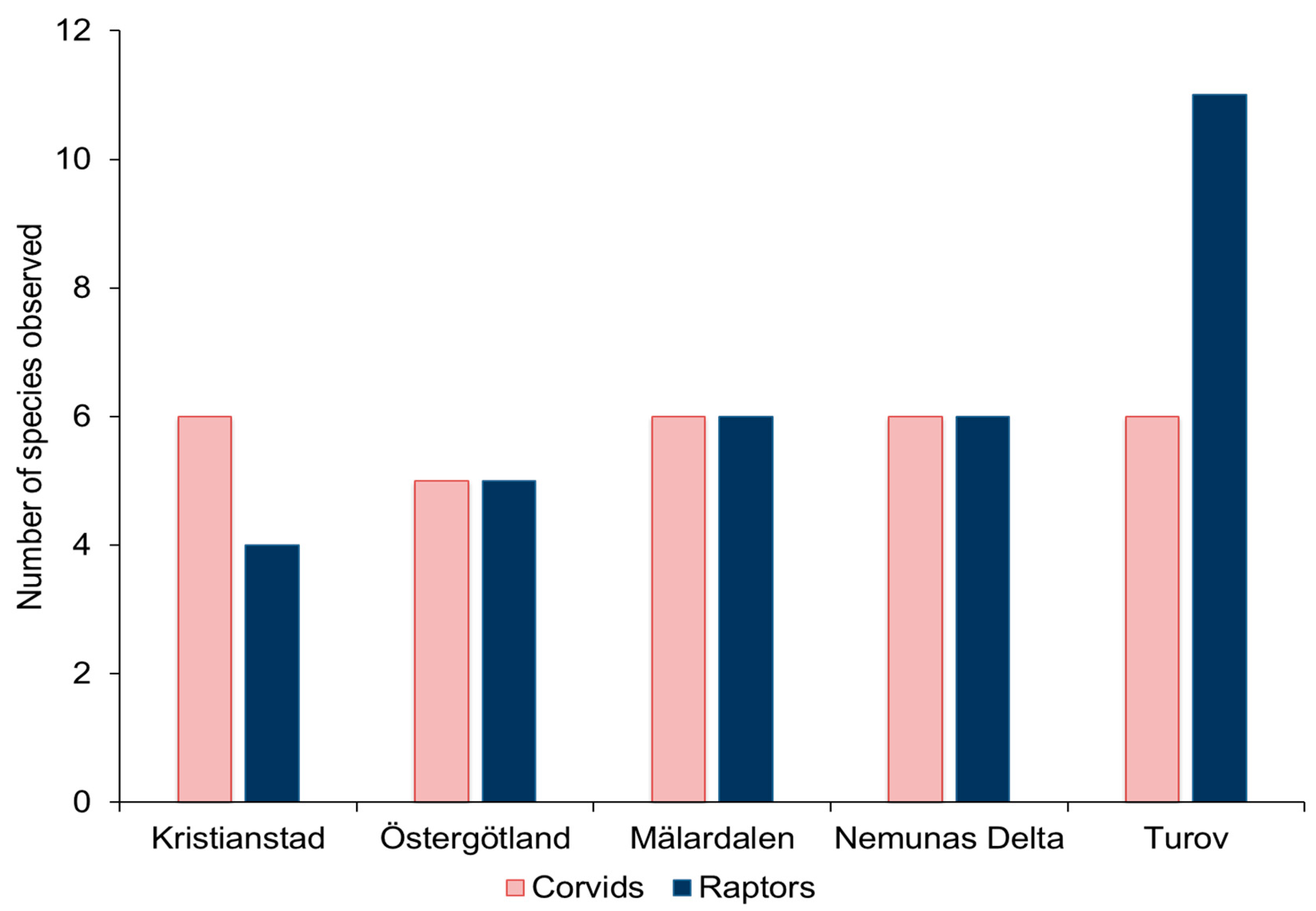
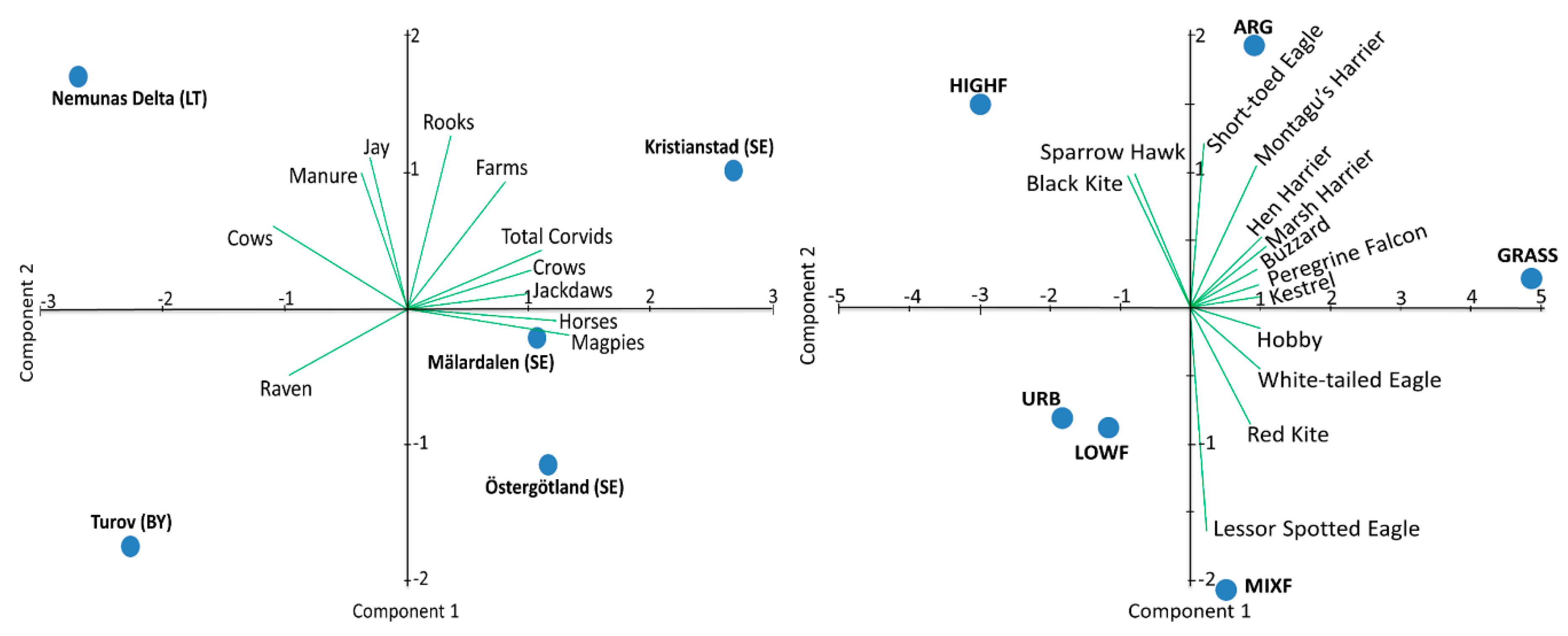
3.1. Avian Predators in Different Landscapes
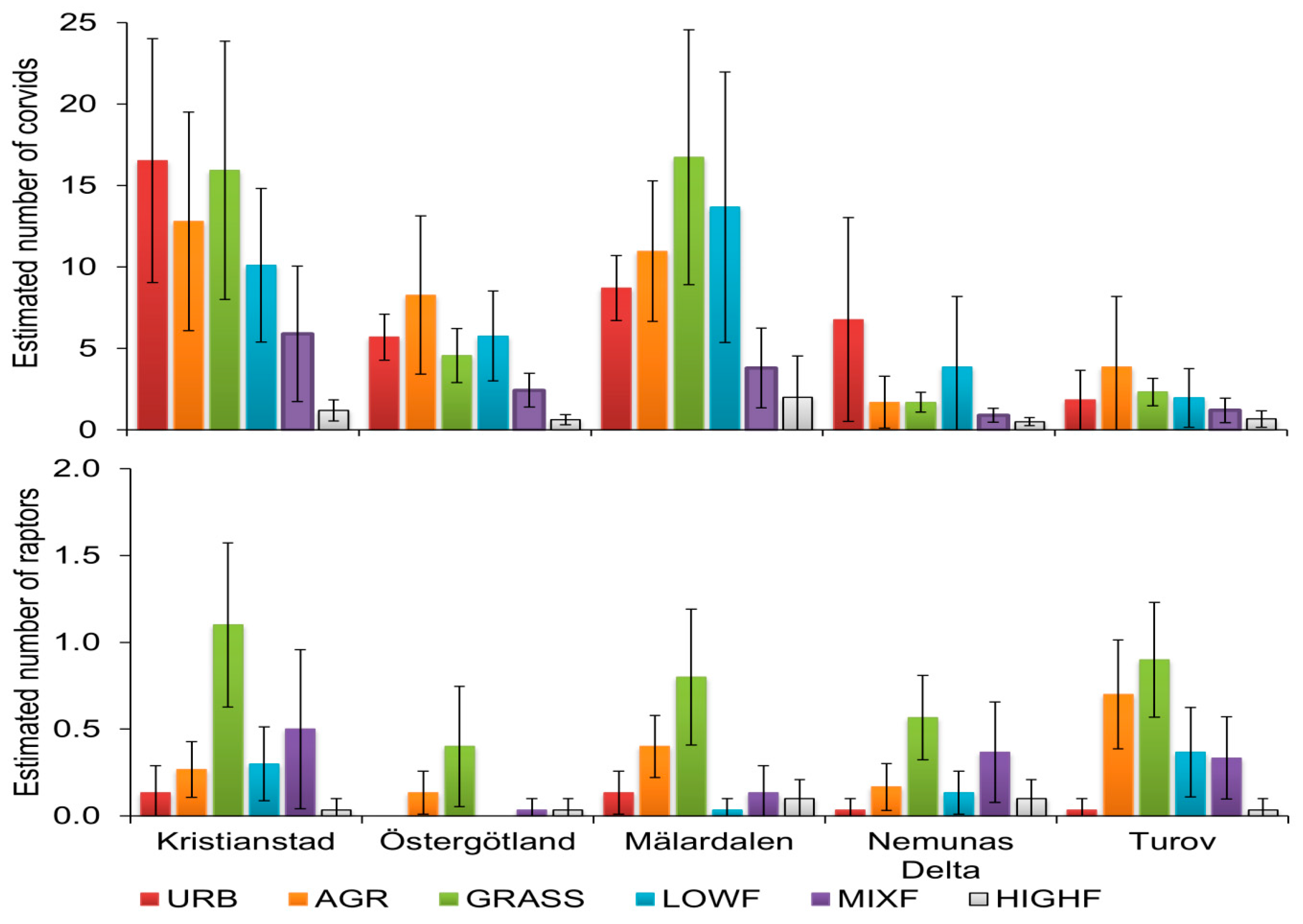
3.2. Avian Predators in Different Landcover Strata
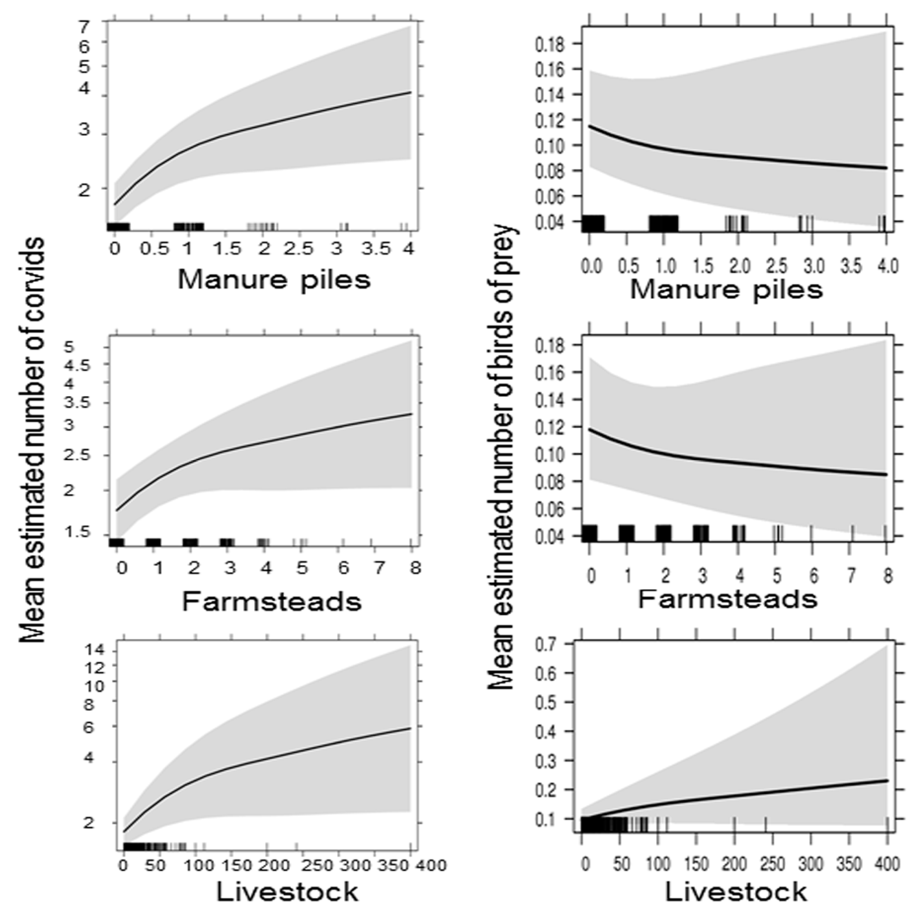
3.3. Avian Predators and Local Resource Abundance
4. Discussion
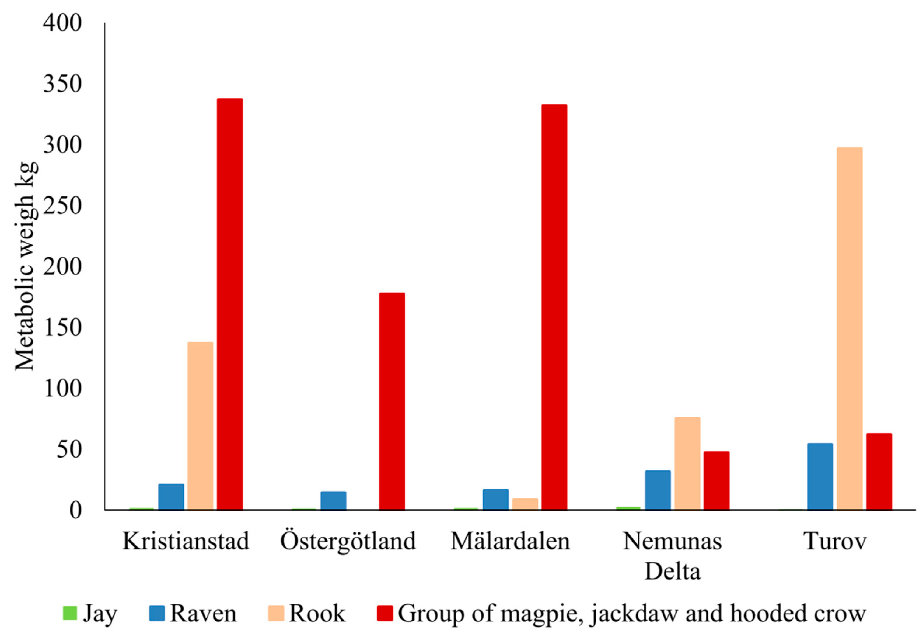
4.1. Omnivorous Corvid Birds and Carnivorous Raptors
4.2. Multi-Scale Management of Patterns and Processes Affecting Habitat Networks
5. Conclusions
Author Contributions
Funding
Acknowledgments
Conflicts of Interest
References
- Butchart, S.H.M.; Walpole, M.; Collen, B.; van Strien, A.; Scharlemann, J.P.W.; Almond, R.E.A.; Baillie, J.E.M.; Bomhard, B.; Brown, C.; Bruno, J.; et al. Global biodiversity: Indicators of recent declines. Science 2010, 328, 1164–1168. [Google Scholar] [CrossRef] [PubMed]
- McCormick, K.; Kautto, N. The Bioeconomy in Europe: An Overview. Sustainability 2013, 5, 2589. [Google Scholar] [CrossRef]
- Angelstam, P.; Dönz-Breuss, M. Measuring forest biodiversity at the stand scale: An evaluation of indicators in European forest history gradients. Ecol. Bull. 2004, 51, 305–332. [Google Scholar]
- Costanza, R.; Cumberland, J.; Daly, H.; Goodland, R.; Norgaard, R.; Kubiszewski, I.; Franco, C. An Introduction to Ecological Economics, 2nd ed.; CRC Press: Boca Raton, FL, USA, 2014. [Google Scholar]
- Jongman, R.H.G.; Bouwma, I.M.; Griffioen, A.; Jones-Walters, L.; Van Doorn, A.M. The Pan European Ecological Network: PEEN. Landsc. Ecol. 2011, 26, 311–326. [Google Scholar] [CrossRef]
- Čivic, K.; Jones-Walters, L. Implementing Green Infrastructure and Ecological Networks in Europe: Lessons Learned and Future Perspectives. J. Green Eng. 2014, 4, 307–324. [Google Scholar]
- European Commission. Green Infrastructure (GI)—Enhancing Europe’s Natural Capital. Communication from the Commission to the European Parliament, the Council, the European Economic and Social Committee and the Committee of the Regions; European Commission: Brussels, Belgium, 2013. [Google Scholar]
- Convention on Biological Diversity. The Strategic Plan for Biodiversity 2011–2020 and the Aichi Biodiversity Target; UNEP: Nagoya, Japan, 2010. [Google Scholar]
- Zulka, K.P.; Abensperg-Traun, M.; Milasowszky, N.; Bieringer, G.; Gereben-Krenn, B.-A.; Holzinger, W.; Hölzler, G.; Rabitsch, W.; Reischütz, A.; Querner, P.; et al. Species richness in dry grassland patches of eastern Austria: A multi-taxon study on the role of local, landscape and habitat quality variables. Agric. Ecosyst. Environ. 2014, 182, 25–36. [Google Scholar] [CrossRef]
- Opdam, P.; Foppen, R.; Reijnen, R.; Schotman, A. The landscape ecological approach in bird conservation: Integrating the metapopulation concept into spatial planning. Ibis 1995, 137, S139–S146. [Google Scholar] [CrossRef]
- Angelstam, P.; Andersson, L. Estimates of the needs for forest reserves in Sweden. Scand. J. For. Res. 2001, 16, 38–51. [Google Scholar] [CrossRef]
- Turner, M.G. Landscape ecology: The effect of pattern on process. Annu. Rev. Ecol. Syst. 1989, 20, 171–197. [Google Scholar] [CrossRef]
- Angelstam, P.; Pedersen, S.; Manton, M.; Garrido, P.; Naumov, V.; Elbakidze, M. Green infrastructure maintenance is more than land cover: Large herbivores limit recruitment of key-stone tree species in Sweden. Landsc. Urban Plan. 2017, 167, 368–377. [Google Scholar] [CrossRef]
- Angelstam, P.; Manton, M.; Pedersen, S.; Elbakidze, M. Disrupted trophic interactions affect recruitment of boreal deciduous and coniferous trees in northern Europe. Ecol. Appl. 2017, 27, 1108–1123. [Google Scholar] [CrossRef] [PubMed]
- Manton, M.; Angelstam, P.; Milberg, P.; Elbakidze, M. Wet meadows as a green infrastructure for ecological sustainability: Wader conservation in Southern Sweden as a case study. Sustainability 2016, 8, 340. [Google Scholar] [CrossRef]
- Berg, Å.; Wretenberg, J.; Żmihorski, M.; Hiron, M.; Pärt, T. Linking occurrence and changes in local abundance of farmland bird species to landscape composition and land-use changes. Agric. Ecosyst. Environ. 2015, 204, 1–7. [Google Scholar] [CrossRef]
- Allan, E.; Manning, P.; Alt, F.; Binkenstein, J.; Blaser, S.; Blüthgen, N.; Böhm, S.; Grassein, F.; Hölzel, N.; Klaus, V.H.; et al. Land use intensification alters ecosystem multifunctionality via loss of biodiversity and changes to functional composition. Ecol. Lett. 2015, 18, 834–843. [Google Scholar] [CrossRef] [PubMed]
- Newey, S.; Mustin, K.; Bryce, R.; Fielding, D.; Redpath, S.; Bunnefeld, N.; Daniel, B.; Irvine, R.J. Impact of Management on Avian Communities in the Scottish Highlands. PLoS ONE 2016, 11, e0155473. [Google Scholar] [CrossRef] [PubMed]
- Angelstam, P.; Roberge, J.M.; Lõhmus, A.; Bergmanis, M.; Brazaitis, G.; Dönz-Breuss, M.; Edenius, L.; Kosinski, Z.; Kurlavicius, P.; Lārmanis, V.; et al. Habitat modelling as a tool for landscape-scale conservation: A review of parameters for focal forest birds. Ecol. Bull. 2004, 51, 427–453. [Google Scholar]
- Laidlaw, R.A.; Smart, J.; Smart, M.A.; Gill, J.A. The influence of landscape features on nest predation rates of grassland-breeding waders. Ibis 2015, 157, 700–712. [Google Scholar] [CrossRef]
- Andrén, H.; Angelstam, P.; Lindström, E.; Widén, P. Differences in predation pressure in relation to habitat fragmentation: An experiment. Oikos 1985, 45, 273–277. [Google Scholar] [CrossRef]
- Lindström, Å.; Green, M.; Husby, M.; Kålås, J.A.; Lehikoinen, A. Large-scale monitoring of waders on their boreal and Arctic breeding grounds in Northern Europe. Ardea 2015, 103, 3–15. [Google Scholar] [CrossRef]
- Thorup, O. Breeding waders in Europe 2000; International Wader Study Group: London, UK, 2005; Volume 14. [Google Scholar]
- Voříšek, P.; Jiguet, F.; van Strien, A.; Škorpilová, J.; Klvaňová, A.; Gregory, R. Trends in abundance and biomass of widespread European farmland birds: How much have we lost. Bou Proc. Lowl. Farml. Birds III 2010, 325, 326–327. [Google Scholar]
- Storch, I. Conservation Status of Grouse Worldwide: An Update. Wildl. Biol. 2007, 13, 5–12. [Google Scholar] [CrossRef]
- Thirgood, S.J.; Redpath, S.M.; Rothery, P.; Aebischer, N.J. Raptor predation and population limitation in red grouse. J. Anim. Ecol. 2000, 69, 504–516. [Google Scholar] [CrossRef]
- BirdLife International. Perdix perdix, 2015; The IUCN Red List of Threatened Species 2015: e.T22678911A59942420. Downloaded on 26 April 2018.
- BirdLife International. Phasianus colchicus, 2016; The IUCN Red List of Threatened Species; 2016: e.T45100023A85926819. [CrossRef]
- Manton, M.; Angelstam, P. Defining Benchmarks for Restoration of Green Infrastructure: A Case Study Combining the Historical Range of Variability of Habitat and Species’ Requirements. Sustainability 2018, 10, 326. [Google Scholar] [CrossRef]
- Batáry, P.; Báldi, A.; Erdős, S. Grassland versus non-grassland bird abundance and diversity in managed grasslands: Local, landscape and regional scale effects. Biodivers. Conserv. 2007, 16, 871–881. [Google Scholar] [CrossRef]
- Żmihorski, M.; Pärt, T.; Gustafson, T.; Berg, Å. Effects of water level and grassland management on alpha and beta diversity of birds in restored wetlands. J. Appl. Ecol. 2016, 53, 587–595. [Google Scholar] [CrossRef]
- Roberge, J.-M.; Angelstam, P.; Villard, M.-A. Specialised woodpeckers and naturalness in hemiboreal forests—Deriving quantitative targets for conservation planning. Biol. Conserv. 2008, 141, 997–1012. [Google Scholar] [CrossRef]
- Törnblom, J.; Angelstam, P.; Degerman, E.; Henrikson, L.; Edman, T.; Temnerud, J. Catchment land cover as a proxy for macroinvertebrate assemblage structure in Carpathian Mountain streams. Hydrobiologia 2011, 673, 153–168. [Google Scholar] [CrossRef]
- Brown, J.H. Macroecology; University of Chicago Press: Chicago, IL, USA, 1995; p. 284. [Google Scholar]
- Smith, F.A.; Gittleman, J.L.; Brown, J.H. Foundations of Macroecology: Classic Papers with Commentaries; University of Chicago Press: Chicago, IL, USA, 2014. [Google Scholar]
- Jepsen, M.R.; Kuemmerle, T.; Müller, D.; Erb, K.; Verburg, P.H.; Haberl, H.; Vesterager, J.P.; Andrič, M.; Antrop, M.; Austrheim, G.; et al. Transitions in European land-management regimes between 1800 and 2010. Land Use Policy 2015, 49, 53–64. [Google Scholar] [CrossRef]
- Naumov, V.; Manton, M.; Elbakidze, M.; Rendenieks, Z.; Priednieks, J.; Uhlianets, S.; Yamelynets, T.; Zhivotovg, A.; Angelstam, P. How to reconcile wood production and biodiversity conservation? The Pan-European boreal forest history gradient as an “experiment”. J. Environ. Manag. 2018, 218, 1–13. [Google Scholar] [CrossRef]
- Popescu, V.D.; Rozylowicz, L.; Niculae, I.M.; Cucu, A.L.; Hartel, T. Species, habitats, society: An evaluation of research supporting EU’s Natura 2000 Network. PLoS ONE 2014, 9, e113648. [Google Scholar] [CrossRef] [PubMed]
- Naumov, V.; Angelstam, P.; Elbakidze, M. Barriers and bridges for intensified wood production in Russia: Insights from the environmental history of a regional logging frontier. For. Policy Econ. 2016, 66, 1–10. [Google Scholar] [CrossRef]
- Puumalainen, J.; Kennedy, P.; Folving, S. Monitoring forest biodiversity: A European perspective with reference to temperate and boreal forest zone. J. Environ. Manag. 2003, 67, 5–14. [Google Scholar] [CrossRef]
- Angelstam, P.; Grodzynskyi, M.; Andersson, K.; Axelsson, R.; Elbakidze, M.; Khoroshev, A.; Kruhlov, I.; Naumov, V. Measurement, collaborative learning and research for sustainable use of ecosystem services: Landscape concepts and Europe as laboratory. Ambio 2013, 42, 129–145. [Google Scholar] [CrossRef] [PubMed]
- Angelstam, P.; Elbakidze, M.; Axelsson, R.; Čupa, P.; Halada, L.; Molnar, Z.; Pătru-Stupariu, I.; Perzanowski, K.; Rozulowicz, L.; Standovar, T.; et al. Maintaining Cultural and Natural Biodiversity in the Carpathian Mountain Ecoregion: Need for an Integrated Landscape Approach. In The Carpathians: Integrating Nature and Society Towards Sustainability; Kozak, J., Ostapowicz, K., Bytnerowicz, A., Wyżga, B., Eds.; Springer: Berlin/Heidelberg, Germany, 2013; pp. 393–424. [Google Scholar]
- Kaczensky, P.; Chapron, G.; Von Arx, M.; Huber, D.; Andrén, H.; Linnell, J. Status, Management and Distribution of Large Carnivores-Bear, Lynx, Wolf & Wolverine in Europe; European Commission: Brussels, Belgium, 2012. [Google Scholar]
- Edman, T.; Angelstam, P.; Mikusiński, G.; Roberge, J.-M.; Sikora, A. Spatial planning for biodiversity conservation: Assessment of forest landscapes’ conservation value using umbrella species requirements in Poland. Landsc. Urban Plan. 2011, 102, 16–23. [Google Scholar] [CrossRef]
- Angelstam, P.; Axelsson, R.; Elbakidze, M.; Laestadius, L.; Lazdinis, M.; Nordberg, M.; Pătru-Stupariu, I.; Smith, M. Knowledge production and learning for sustainable forest management on the ground: Pan-European landscapes as a time machine. Forestry 2011, 84, 581–596. [Google Scholar] [CrossRef]
- Hall, L.S.; Krausman, P.R.; Morrison, M.L. The habitat concept and a plea for standard terminology. Wildl. Soc. Bull. 1997, 25, 173–182. [Google Scholar]
- Wiens, J.A. Spatial scaling in ecology. Funct. Ecol. 1989, 3, 385–397. [Google Scholar] [CrossRef]
- Forman, R.T. Some general principles of landscape and regional ecology. Landsc. Ecol. 1995, 10, 133–142. [Google Scholar] [CrossRef]
- Dunning, J.B.; Danielson, B.J.; Pulliam, H.R. Ecological processes that affect populations in complex landscapes. Oikos 1992, 65, 169–175. [Google Scholar] [CrossRef]
- Poiani, K.A.; Richter, B.D.; Anderson, M.G.; Richter, H.E. Biodiversity Conservation at Multiple Scales: Functional Sites, Landscapes, and Networks. BioScience 2000, 50, 133–146. [Google Scholar] [CrossRef]
- Beck, J.; Ballesteros-Mejia, L.; Buchmann, C.M.; Dengler, J.; Fritz, S.A.; Gruber, B.; Hof, C.; Jansen, F.; Knapp, S.; Kreft, H.; et al. What’s on the horizon for macroecology? Ecography 2012, 35, 673–683. [Google Scholar] [CrossRef]
- Plieninger, T.; Kizos, T.; Bieling, C.; Le Dû-Blayo, L.; Budniok, M.-A.; Bürgi, M.; Crumley, C.L.; Girod, G.; Howard, P.; Kolen, J. Exploring ecosystem-change and society through a landscape lens: Recent progress in European landscape research. Ecol. Soc. 2015, 20, 5. [Google Scholar] [CrossRef]
- Manton, M. Managing Green Infrastructures: Trophic Interactions in Anthropogenic and Natural Ecosystems; (Licentiate); Swedish University of Agricultural Sciences: Kaunas, Lithuania, 2014. [Google Scholar]
- Gunst, P. Agrarian systems of central and eastern Europe. In The Origins of Backwardness in Eastern Europe: Economics and Politics from the Middle Ages until the Early Twentieth Century; Chirot, D., Ed.; California University Press: Berkeley, CA, USA, 1989; pp. 53–91. [Google Scholar]
- Žalakevičius, M. Global climate change impact on bird Numbers, population state and distribution areas. Acta Zool. Litu. 1999, 9, 78–89. [Google Scholar] [CrossRef]
- Angelstam, P.; Naumov, V.; Elbakidze, M.; Manton, M.; Priednieks, J.; Rendenieks, Z. Wood production and biodiversity conservation are rival forestry objectives in Europe’s Baltic Sea Region. Ecosphere 2018, 9, e02119. [Google Scholar] [CrossRef]
- Eisenhardt, K.M. Building theories from case study research. Acad. Manag. Rev. 1989, 14, 532–550. [Google Scholar] [CrossRef]
- Flyvbjerg, B. Case Study. In The Sage Handbook of Qualative Research, 4th ed.; Denzin, N.K., Lincoln, Y.S., Eds.; Sage: Thousand Oaks, CA, USA, 2011; pp. 301–316. [Google Scholar]
- Berglund, B.E. Palaeoecology. Ecol. Bull. 1991, 41, 31–35. [Google Scholar]
- Ericsson, S.; Östlund, L.; Axelsson, A.-L. A forest of grazing and logging: Deforestation and reforestation history of a boreal landscape in central Sweden. New For. 2000, 19, 227–240. [Google Scholar] [CrossRef]
- Eriksson, O.; Cousins, S. Historical landscape perspectives on grasslands in Sweden and the Baltic Region. Land 2014, 3, 300. [Google Scholar] [CrossRef]
- Lindström, Å.; Green, M. Monitoring Population Changes of Birds in Sweden. Annual Report for 2012; Department of Biology, Lund University: Lund, Sweden, 2013; 80p. [Google Scholar]
- Ödman, A.M.; Olsson, P.A. Conservation of sandy calcareous grassland: What can be learned from the land use history? PLoS ONE 2014, 9, e90998. [Google Scholar] [CrossRef]
- Magnusson, S.-E.; Magntorn, K.; Wallsten, E.; Cronert, H.; Thelaus, M. Kristianstads Vattenrike Biosphere Reserve Nomination Form; Kristianstad Kommun: Kristianstad, Sweden, 2004. [Google Scholar]
- Brukas, V. New World, Old Ideas—A Narrative of the Lithuanian Forestry Transition. J. Environ. Policy Plan. 2015, 17, 495–515. [Google Scholar] [CrossRef]
- Rashleigh, B.; Razinkovas, A.; Pilkaitytė, R. Ecosystem services assessment of the Nemunas River delta. Transit. Waters Bull. 2012, 5, 75–84. [Google Scholar]
- Kurlavičius, P. Lithuanian breeding bird atlas. In Lithuanian Ornithological Society; Lututė: Kaunas, Lithuania, 2006. [Google Scholar]
- Raudonikis, L. Important Bird Areas of the European Union Importance in Lithuania; Lutute: Kaunas, Lithuania, 2004. [Google Scholar]
- Republic of Belarus. Statistical Year Book of the Republic of Belarus 2004; BelStat: Minsk, Belarus, 2004. [Google Scholar]
- Benstead, P.; Jose, P.; Joyce, C.; Wade, P. European Wet Grassland: Guidelines for Management and Restoration; RSPB Sandy: Bedfordshire, UK, 1999. [Google Scholar]
- Pinchuk, P.; Karlionova, N.; Zhurauliou, D. Wader ringing at the Turov ornithological station, Pripyat Valley (S Belarus) in 1996–2003. Ring 2005, 27, 101. [Google Scholar] [CrossRef]
- Yatsukhno, V. Biological and Landscape Diversity Conservation as a Key to Sustainable Agricultural Development of Belarusian Polesye; Academy: Brest, France, 2006. [Google Scholar]
- O’Neill, R.V.; Milne, B.T.; Turner, M.G.; Gardner, R.H. Resource utilization scales and landscape pattern. Landsc. Ecol. 1988, 2, 63–69. [Google Scholar] [CrossRef]
- Gardner, R.H.; Turner, M.G.; O’Neill, R.V.; Lavorel, S. Simulation of the Scale-Dependent Effects of Landscape Boundaries on Species Persistence and Dispersal. In Ecotones: The Role of Landscape Boundaries in the Management and Restoration of Changing Environments; Holland, M.M., Risser, P.G., Naiman, R.J., Eds.; Springer: Boston, MA, USA, 1991; pp. 76–89. [Google Scholar]
- Fahrig, L. Effects of habitat fragmentation on biodiversity. Annu. Rev. Ecol. Evol. Syst. 2003, 34, 487–515. [Google Scholar] [CrossRef]
- ESRI. ArcGIS Desktop: Release 10.1; Environmental Systems Research Institute: Redlands, CA, USA, 2012. [Google Scholar]
- European Environment Agency. Landscapes in Transition: An Account of 25 Years of Land Cover Change in Europe; European Commission: Luxembourg City, Luxembourg, 2017. [Google Scholar]
- Arino, O.; Ramos Perez, J.J.; Kalogirou, V.; Bontemps, S.; Defourny, P.; Van Bogaert, E. Global Land Cover Map for 2009 (GlobCover 2009); PANGAEA: Frascati, Italy, 2012. [Google Scholar]
- Rannap, R.; Kaart, T.; Pehlak, H.; Kana, S.; Soomets, E.; Lanno, K. Coastal meadow management for threatened waders has a strong supporting impact on meadow plants and amphibians. J. Nat. Conserv. 2017, 35, 77–91. [Google Scholar] [CrossRef]
- Marzluff, J.M.; Neatherlin, E. Corvid response to human settlements and campgrounds: Causes, consequences, and challenges for conservation. Biol. Conserv. 2006, 130, 301–314. [Google Scholar] [CrossRef]
- Andrén, H.; Angelstam, P. Elevated predation rates as an edge effect in habitat islands: Experimental evidence. Ecology 1988, 69, 544–547. [Google Scholar] [CrossRef]
- Cramp, S.; Perrins, C.M.; Brooks, D.J. Handbook of the Birds of Europe, the Middle East, and North Africa: The Birds of the Western Palearctic. Vol. 8, Crows to Finches; Oxford University Press: Oxford, UK, 1980. [Google Scholar]
- Cramp, S. Handbook of the Birds of Europe, the Middle East, and North Africa: The Birds of the Western Palearctic. Vol. 2, Hawks to Bustards; Oxford University Press: Oxford, UK, 1980. [Google Scholar]
- Rullman, S.; Marzluff, J.M. Raptor Presence Along an Urban–Wildland Gradient: Influences of Prey Abundance and Land Cover. J. Raptor Res. 2014, 48, 257–272. [Google Scholar] [CrossRef]
- Fox, J. Applied Regression Analysis and Generalized Linear Models; Sage Publications: London, UK, 2015. [Google Scholar]
- R Core Team. R: A Language and Environment for Statistical Computing; R Foundation for Statistical Computing: Vienna, Austria, 2016; Available online: https://www.R-project.org/ (accessed on 29 April 2019).
- Bates, D.; Maechler, M.; Bolker, B.M.; Walker, S.C. Fitting Linear Mixed-Effects Models Using lme4. J. Stat. Softw. 2015, 67, 1–48. [Google Scholar] [CrossRef]
- Zuur, A.F.; Ieno, E.N.; Walker, N.L.; Saveliev, A.A.; Smith, G.M. Mixed Effects Models and Extensions in Ecology with R; Springer: New York, NY, USA, 2009. [Google Scholar]
- Lasiewski, R.C.; Dawson, W.R. A re-examination of the relation between standard metabolic rate and body weight in birds. Condor 1967, 69, 13–23. [Google Scholar] [CrossRef]
- Jorgenson, A.K.; Alekseyko, A.; Giedraitis, V. Energy consumption, human well-being and economic development in central and eastern European nations: A cautionary tale of sustainability. Energy Policy 2014, 66, 419–427. [Google Scholar] [CrossRef]
- Dombrovski, V.C.; Ivanovski, V.V. New Data on Numbers and Distribution of Birds of Prey Breeding in Belarus. Acta Zool. Litu. 2005, 15, 218–227. [Google Scholar] [CrossRef]
- Ottvall, R.; Edenius, L.; Elmberg, J.; Engström, H.; Green, M.; Holmqvist, N.; Lindström, Å.; Pärt, T.; Tjernberg, M. Population trends for Swedish breeding birds. Ornis Svec. 2009, 19, 117–192. [Google Scholar]
- Nikiforov, M. Distribution Trends of Breeding Bird Species in Belarus under Conditions of Global Climate Change. Acta Zool. Litu. 2003, 13, 255–262. [Google Scholar] [CrossRef]
- Devictor, V.; Julliard, R.; Jiguet, F. Distribution of specialist and generalist species along spatial gradients of habitat disturbance and fragmentation. Oikos 2008, 117, 507–514. [Google Scholar] [CrossRef]
- Marzluff, J.M.; Angell, T. Cultural coevolution: How the human bond with crows and ravens extends theory and raises new questions. J. Ecol. Anthropol. 2005, 9, 69–75. [Google Scholar] [CrossRef]
- Krojerová-Prokešová, J.; Homolka, M.; Barančeková, M.; Heroldová, M.; Baňař, P.; Kamler, J.; Purchart, L.; Suchomel, J.; Zejda, J. Structure of small mammal communities on clearings in managed Central European forests. For. Ecol. Manag. 2016, 367, 41–51. [Google Scholar] [CrossRef]
- Bowman, J.; Forbes, G.; Dilworth, T. Landscape context and small-mammal abundance in a managed forest. For. Ecol. Manag. 2001, 140, 249–255. [Google Scholar] [CrossRef]
- Churchfield, S.; Hollier, J.; Brown, V.K. Community structure and habitat use of small mammals in grasslands of different successional age. J. Zool. 1997, 242, 519–530. [Google Scholar] [CrossRef]
- Stighäll, K.; Roberge, J.-M.; Andersson, K.; Angelstam, P. Usefulness of biophysical proxy data for modelling habitat of an endangered forest species: The white-backed woodpecker Dendrocopos leucotos. Scand. J. For. Res. 2011, 26, 576–585. [Google Scholar] [CrossRef]
- Benstead, P.; Drake, M.; Jose, P.; Mountford, O.; Newbold, C.; Treweek, J. The Wet Grassland Guide; Royal Society for the Protection of Birds: Sandy, UK, 1997. [Google Scholar]
- Naiman, R.J.; Bechtold, J.S.; Drake, D.C.; Latterell, J.J.; O’Keefe, T.C.; Balian, E.V. Origins, Patterns, and Importance of Heterogeneity in Riparian Systems. In Ecosystem Function in Heterogeneous Landscapes; Lovett, G.M., Turner, M.G., Jones, C.G., Weathers, K.C., Eds.; Springer: New York, NY, USA, 2005; pp. 279–309. [Google Scholar]
- Joyce, C.; Wade, P. Wet Grasslands: A European Perspective; John Wiley: Chichester, UK, 1998; p. 340. [Google Scholar]
- Price, E. Lowland Grassland and Heathland Habitats; Routledge: London, UK, 2003. [Google Scholar]
- Panzacchi, M.; Linnell, J.D.C.; Melis, C.; Odden, M.; Odden, J.; Gorini, L.; Andersen, R. Effect of land-use on small mammal abundance and diversity in a forest–farmland mosaic landscape in south-eastern Norway. For. Ecol. Manag. 2010, 259, 1536–1545. [Google Scholar] [CrossRef]
- Newton, I.; Davis, P.E.; Davis, J.E. Ravens and Buzzards in Relation to Sheep-Farming and Forestry in Wales. J. Appl. Ecol. 1982, 19, 681–706. [Google Scholar] [CrossRef]
- Fuller, R.J. Relationships between Grazing and Birds with Particular Reference to Sheep in the British Uplands. British Trust for Ornithology; British Trust for Ornithology: Norfolk, UK, 1996; p. 94. [Google Scholar]
- Statistics Sweden. Yearbook of Agriculture Statistics 2013; SCB: Örebro, Sweden, 2013.
- Cunha, T.J. Horse Feeding and Nutrition, 2nd ed.; Academic Press: London, UK, 2012. [Google Scholar]
- Parvage, M. Impact of Horse-Keeping on Phosphorus (P) Concentrations in Soil and Water. Ph.D. Thesis, Swedish University of Agricultural Sciences, Uppsala, Sweden, 2015. [Google Scholar]
- Kentie, R.; Both, C.; Hooijmeijer, J.C.E.W.; Piersma, T. Management of modern agricultural landscapes increases nest predation rates in Black-tailed Godwits Limosa limosa. Ibis 2015, 157, 614–625. [Google Scholar] [CrossRef]
- Amar, A.; Thirgood, S.; Pearce-Higgins, J.; Redpath, S. The impact of raptors on the abundance of upland passerines and waders. Oikos 2008, 117, 1143–1152. [Google Scholar] [CrossRef]
- Angelstam, P. Predation on ground-nesting birds’ nests in relation to predator densities and habitat edge. Oikos 1986, 47, 365–373. [Google Scholar] [CrossRef]
- Roodbergen, M.; Werf, B.; Hötker, H. Revealing the contributions of reproduction and survival to the Europe-wide decline in meadow birds: Review and meta-analysis. J. Ornithol. 2011, 153, 53–74. [Google Scholar] [CrossRef]
- Andrén, H. Corvid density and nest predation in relation to forest fragmentation: A landscape perspective. Ecology 1992, 73, 794–804. [Google Scholar] [CrossRef]
- Summers, R.W.; Green, R.E.; Proctor, R.; Dugan, D.; Lambie, D.; Moncrieff, R.; Moss, R.; Baines, D. An experimental study of the effects of predation on the breeding productivity of capercaillie and black grouse. J. Appl. Ecol. 2004, 41, 513–525. [Google Scholar] [CrossRef]
- Green, R.E.; Hawell, J.; Johnson, T.H. Identification of predators of wader eggs from egg remains. Bird Study 1987, 34, 87–91. [Google Scholar] [CrossRef]
- Macdonald, M.A.; Bolton, M. Predation on wader nests in Europe. Ibis 2008, 150, 54–73. [Google Scholar] [CrossRef]
- Jongman, R.H.G. Nature conservation planning in Europe: Developing ecological networks. Landsc. Urban Plan. 1995, 32, 169–183. [Google Scholar] [CrossRef]
- Van den Berg, L.J.L.; Tomassen, H.B.M.; Roelofs, J.G.M.; Bobbink, R. Effects of nitrogen enrichment on coastal dune grassland: A mesocosm study. Environ. Pollut. 2005, 138, 77–85. [Google Scholar] [CrossRef] [PubMed]
- Dahlström, A. Grazing dynamics at different spatial and temporal scales: Examples from the Swedish historical record a.d. 1620–1850. Veg. Hist. Archaeobotany 2008, 17, 563–572. [Google Scholar]
- Triviño, M.; Juutinen, A.; Mazziotta, A.; Miettinen, K.; Podkopaev, D.; Reunanen, P.; Mönkkönen, M. Managing a boreal forest landscape for providing timber, storing and sequestering carbon. Ecosyst. Serv. 2015, 14, 179–189. [Google Scholar] [CrossRef]
- Mönkkönen, M.; Juutinen, A.; Mazziotta, A.; Miettinen, K.; Podkopaev, D.; Reunanen, P.; Salminen, H.; Tikkanen, O.-P. Spatially dynamic forest management to sustain biodiversity and economic returns. J. Environ. Manag. 2014, 134, 80–89. [Google Scholar] [CrossRef] [PubMed]


| Case Study Landscape from West to East | Sweden | Lithuania | Belarus | ||
|---|---|---|---|---|---|
| Kristianstad | Östergötland | Mälardalen | Nemunas Delta | Turov | |
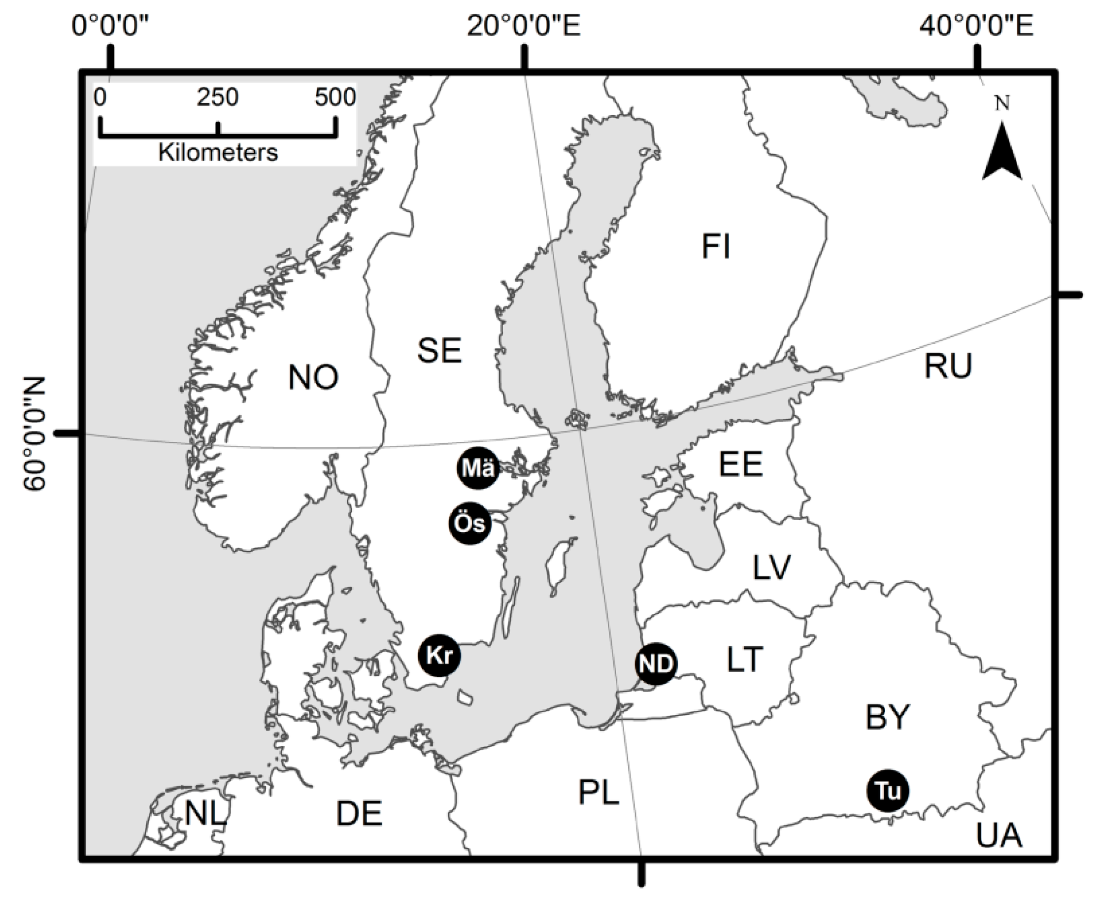
| Latitude | 55°59′ N | 58°25′ N | 59°50′ N | 55°18′ N | 52°4′ N |
| Longitude | 14°12′ E | 15°35′ E | 16°20′ E | 21°20′ E | 27°44′ E |
| Area km2 | 1370 | 2146 | 2028 | 1318 | 1349 |
| Biogeographical region | Temperate | Hemiboreal | Hemiboreal | Hemiboreal | Temperate |
| Population density (n/km2) | 45 | 40 | 39 | 30 | 16 |
| Population change 1965–2015 | 1.40 | 1.22 | 1.07 | 0.74 | 0.58 |
| GDP per capita | 37648 | 39000 | 37492 | 30501 | 18804 |
| Dominating focal and other landcovers (%) | |||||
| Urban areas (URB) | 4.3 | 2.5 | 2.2 | 0.3 | 0.5 |
| Agricultural land (AGR) | 34.3 | 28.6 | 26.0 | 33.9 | 16.9 |
| Semi-natural grassland (GRASS) | 1.3 | 0.5 | 1.0 | 31.7 | 37.1 |
| Low forest (LOWF) | 15.7 | 21.9 | 18.2 | 7.7 | 14.2 |
| Mixed forest (MIXF) | 11.5 | 13.6 | 14.1 | 7.0 | 7.2 |
| High forest (HIGHF) | 6. 7 | 15.4 | 15.2 | 4.5 | 5.8 |
| Other | 32.9 | 17.5 | 23.3 | 14.9 | 18.3 |
| Total | 100 | 100 | 100 | 100 | 100 |

| Case Study Landscapes from West to East | ||||||
|---|---|---|---|---|---|---|
| Sweden | Lithuania | Belarus | ||||
| Type of variable | Kristianstad | Östergötland | Mälardalen | Nemunas Delta | Turov | |
| Dependent | Corvid birds | 10.41 ± 1.25 | 4.56 ± 0.54 | 9.31 ± 1.14 | 2.57 ± 0.67 | 1.97 ± 0.43 |
| Raptors | 0.38 ± 0.06 | 0.1 ± 0.03 | 0.26 ± 0.04 | 0.22 ± 0.39 | 0.39 ± 0.05 | |
| Independent | Livestock | 6.26 ± 1.08 | 3.74 ± 0.84 | 4.46 ± 0.81 | 10.30 ± 1.31 | 8.01 ± 2.95 |
| Horses | 0.63 ± 0.11 | 0.58 ± 0.16 | 0.46 ± 0.12 | 0.22 ± 0.06 | 0.26 ± 0.05 | |
| Cows | 4.29 ± 0.93 | 3.04 ± 0.83 | 3.67 ± 0.77 | 10.07 ± 1.30 | 7.64 ± 2.95 | |
| Sheep | 0.92 ± 0.37 | 0.13 ± 0.09 | 0.33 ± 0.21 | 0.01 ± 0.01 | 0.08 ± 0.08 | |
| Farms | 0.89 ± 0.09 | 0.97 ± 0.08 | 0.60 ± 0.06 | 0.78 ± 0.09 | 0.12 ± 0.03 | |
| Manure | 0.18 ± 0.04 | 0.07 ± 0.02 | 0.19 ± 0.04 | 0.28 ± 0.05 | 0.12 ± 0.03 | |
| Recreational areas | 0.27 ± 0.03 | 0.26 ± 0.03 | 0.17 ± 0.03 | 0.10 ± 0.02 | 0.02 ± 0.01 | |
| Corvids | Raptors | |||||
|---|---|---|---|---|---|---|
| Regressor | Chi-Square Test | Df | p-Value | Chi-Square Test | Df | p-Value |
| Landscape | 189.5 | 4 | <2.2 × 10⁻¹⁶ *** | 25.6 | 4 | 3.8 × 10⁻⁵ *** |
| Landcover strata | 163.1 | 5 | <2.2 × 10⁻¹⁶ *** | 82.6 | 5 | 2.3 × 10⁻¹⁶ *** |
| Landscape and landcover strata | 36.1 | 20 | 0.015 * | −1.84 | 20 | 0.091 |
| Manure (sqrt) | 8.3 | 1 | 0.004 ** | −0.08 | 1 | 0.649 |
| Farms (sqrt) | 4.1 | 1 | 0.044 * | −0.07 | 1 | 0.596 |
| Total Stock (sqrt) | 5.1 | 1 | 0.025 * | 0.04 | 1 | 0.127 |
| Horses | 3.9 | 1 | 0.046 * | - | - | - |
| Cows | 4.1 | 1 | 0.044 * | - | - | - |
| Corvids | PCA 1 | PCA 2 | Raptors | PC 1 | PC 2 |
|---|---|---|---|---|---|
| Jackdaw | 0.80 | 0.02 | White-tailed Eagle | 0.31 | −0.12 |
| Crow | 0.79 | 0.16 | Lesser Spotted Eagle | 0.06 | −0.60 |
| Raven | −0.76 | −0.28 | Short-toed Eagle | 0.04 | 0.41 |
| Rook | 0.24 | 0.67 | Red Kite | 0.32 | −0.26 |
| Magpie | 0.89 | −0.07 | Black Kite | −0.19 | 0.31 |
| Jay | −0.27 | 0.90 | Marsh Harrier | 0.35 | 0.16 |
| Horses | 0.97 | −0.09 | Hen Harrier | 0.34 | 0.19 |
| Cows | −0.88 | 0.41 | Montagu’s Harrier | 0.28 | 0.36 |
| Manure | −0.31 | 0.86 | Buzzard | 0.32 | 0.09 |
| Farms | 0.24 | 0.33 | Sparrowhawk | −0.19 | 0.31 |
| Corvids Total | 0.58 | 0.53 | Kestrel | 0.32 | 0.03 |
| Hobby | 0.31 | −0.06 | |||
| Peregrine Falcon | 0.32 | 0.05 |
© 2019 by the authors. Licensee MDPI, Basel, Switzerland. This article is an open access article distributed under the terms and conditions of the Creative Commons Attribution (CC BY) license (http://creativecommons.org/licenses/by/4.0/).
Share and Cite
Manton, M.; Angelstam, P.; Naumov, V. Effects of Land Use Intensification on Avian Predator Assemblages: A Comparison of Landscapes with Different Histories in Northern Europe. Diversity 2019, 11, 70. https://doi.org/10.3390/d11050070
Manton M, Angelstam P, Naumov V. Effects of Land Use Intensification on Avian Predator Assemblages: A Comparison of Landscapes with Different Histories in Northern Europe. Diversity. 2019; 11(5):70. https://doi.org/10.3390/d11050070
Chicago/Turabian StyleManton, Michael, Per Angelstam, and Vladimir Naumov. 2019. "Effects of Land Use Intensification on Avian Predator Assemblages: A Comparison of Landscapes with Different Histories in Northern Europe" Diversity 11, no. 5: 70. https://doi.org/10.3390/d11050070
APA StyleManton, M., Angelstam, P., & Naumov, V. (2019). Effects of Land Use Intensification on Avian Predator Assemblages: A Comparison of Landscapes with Different Histories in Northern Europe. Diversity, 11(5), 70. https://doi.org/10.3390/d11050070