After the Fall: Legacy Effects of Biogenic Structure on Wind-Generated Ecosystem Processes Following Mussel Bed Collapse


Abstract
:
1. Introduction
2. Materials and Methods
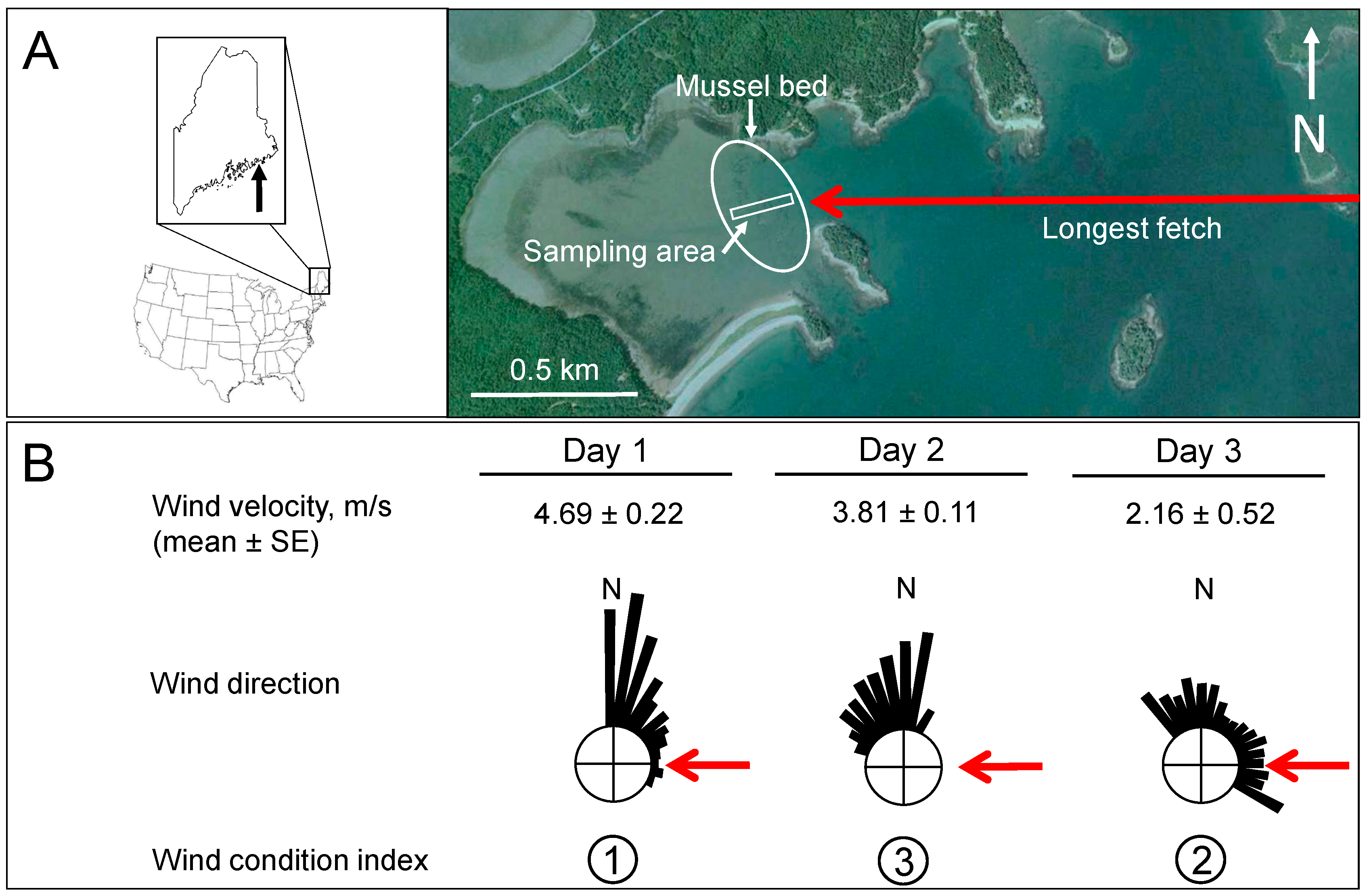
2.1. Study Site
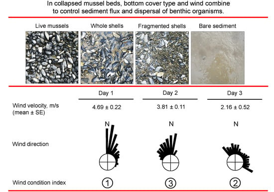
2.2. Wind Condition
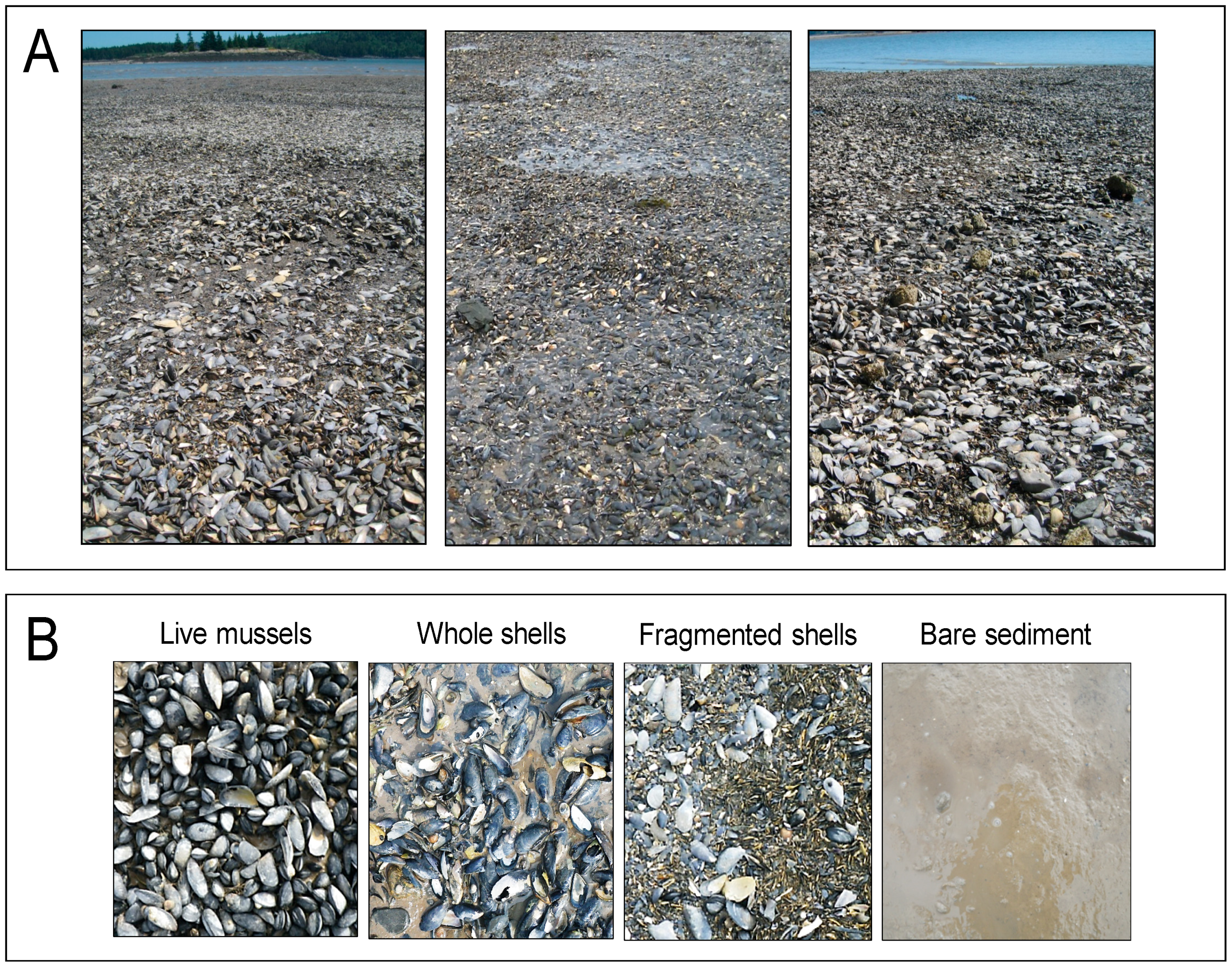
2.3. Field and Laboratory Procedures
- Sediment flux rate = g sediment trap−1 d−1
- Absolute dispersal rate (ADR) = number of individuals trap−1 d−1
- Relative dispersal rate (RDR) = number of individuals trap−1 d−1 ambient individual−1, calculated by dividing the number of individuals collected in a trap by the number of individuals collected in the core from the same location. Relative dispersal rate normalizes for ambient density. It is equivalent to per capita dispersal. For example, RDR > 1 occurs when the number of individuals in a trap is larger than the number of individuals in its corresponding core. Note that in some cases the number of macrofauna individuals in a core = 0, so RDR was undefined due to the 0 in the denominator. Those samples could not be used, resulting in unequal sample sizes. Our statistical analysis relied on a balanced design, so RDR was not calculated for macrofauna.
- Bulk dispersal rate (BDR) = number of individuals g sediment−1 trap−1 d−1, calculated by dividing the number of individuals collected in a trap by the sediment mass collected in that trap. It is a measure of dispersal per unit of transported sediment, providing information on how tightly linked animal movement is to passive bedload transport.
2.4. Data Analysis
3. Results
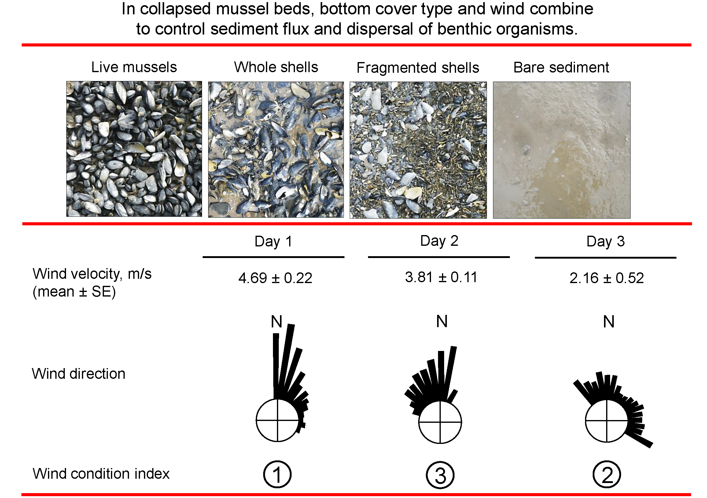
3.1. Sediment
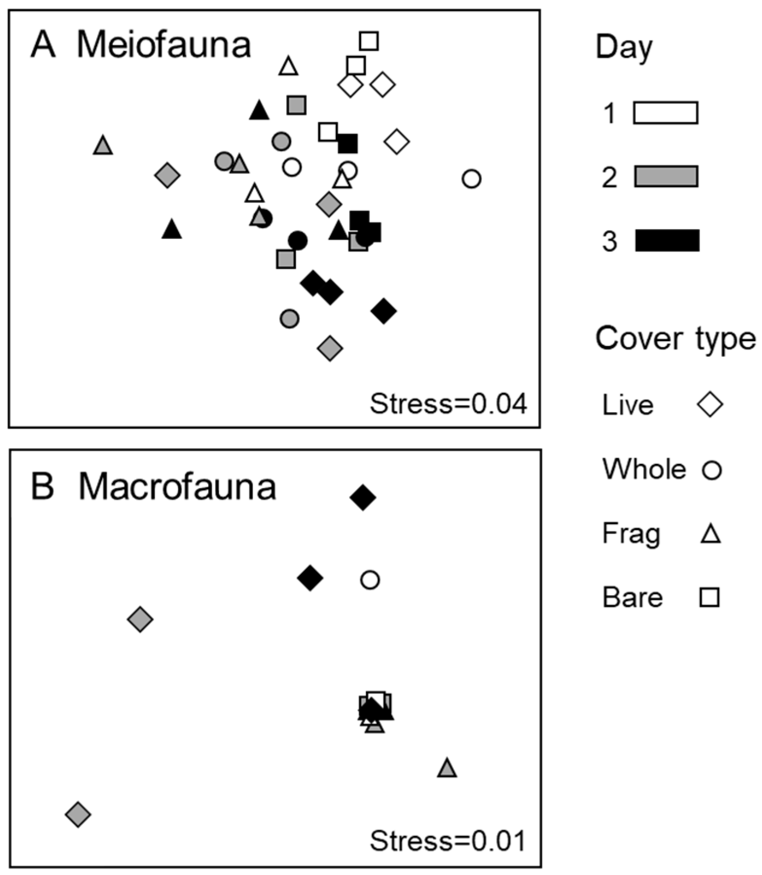
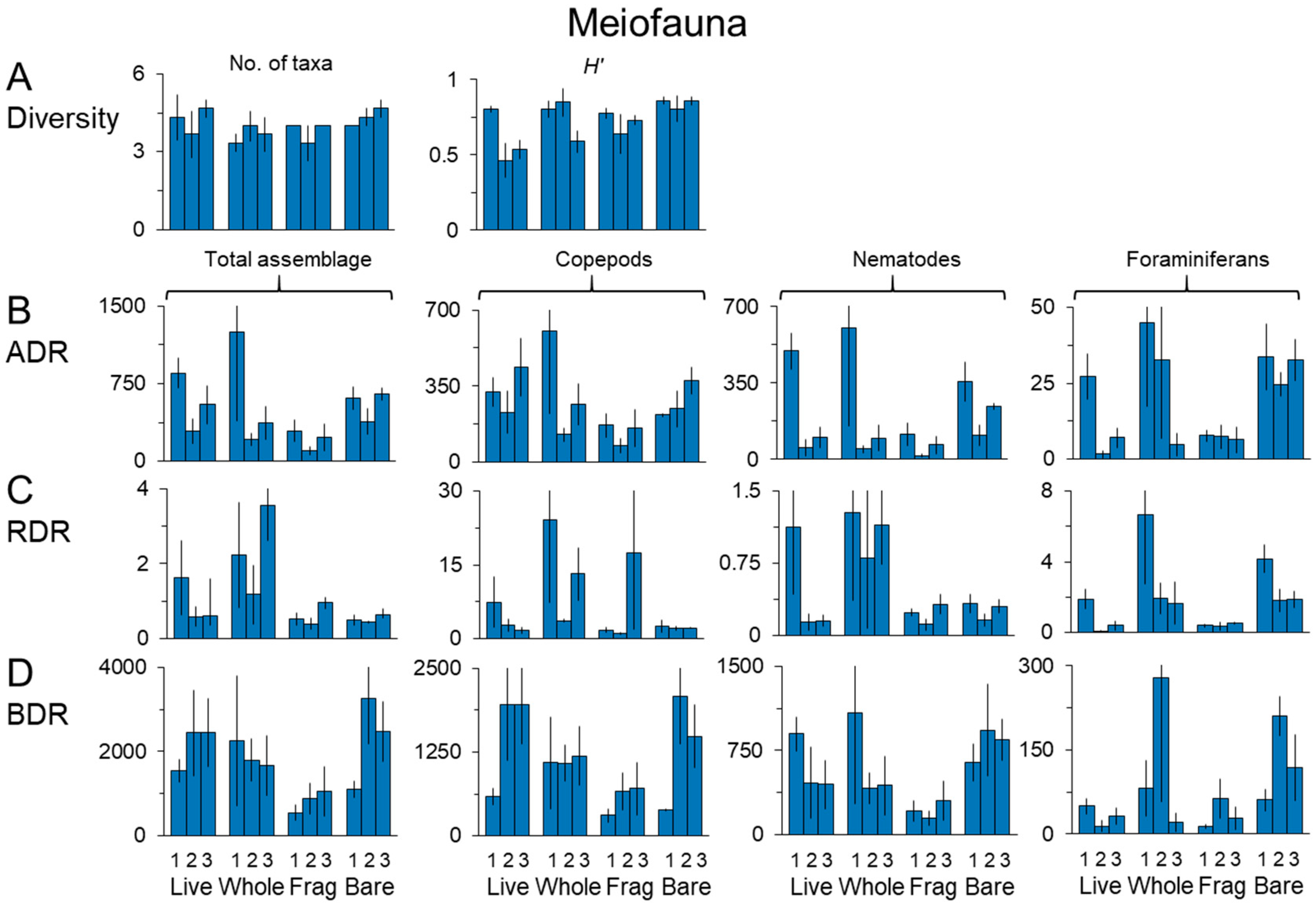
3.2. Meiofauna
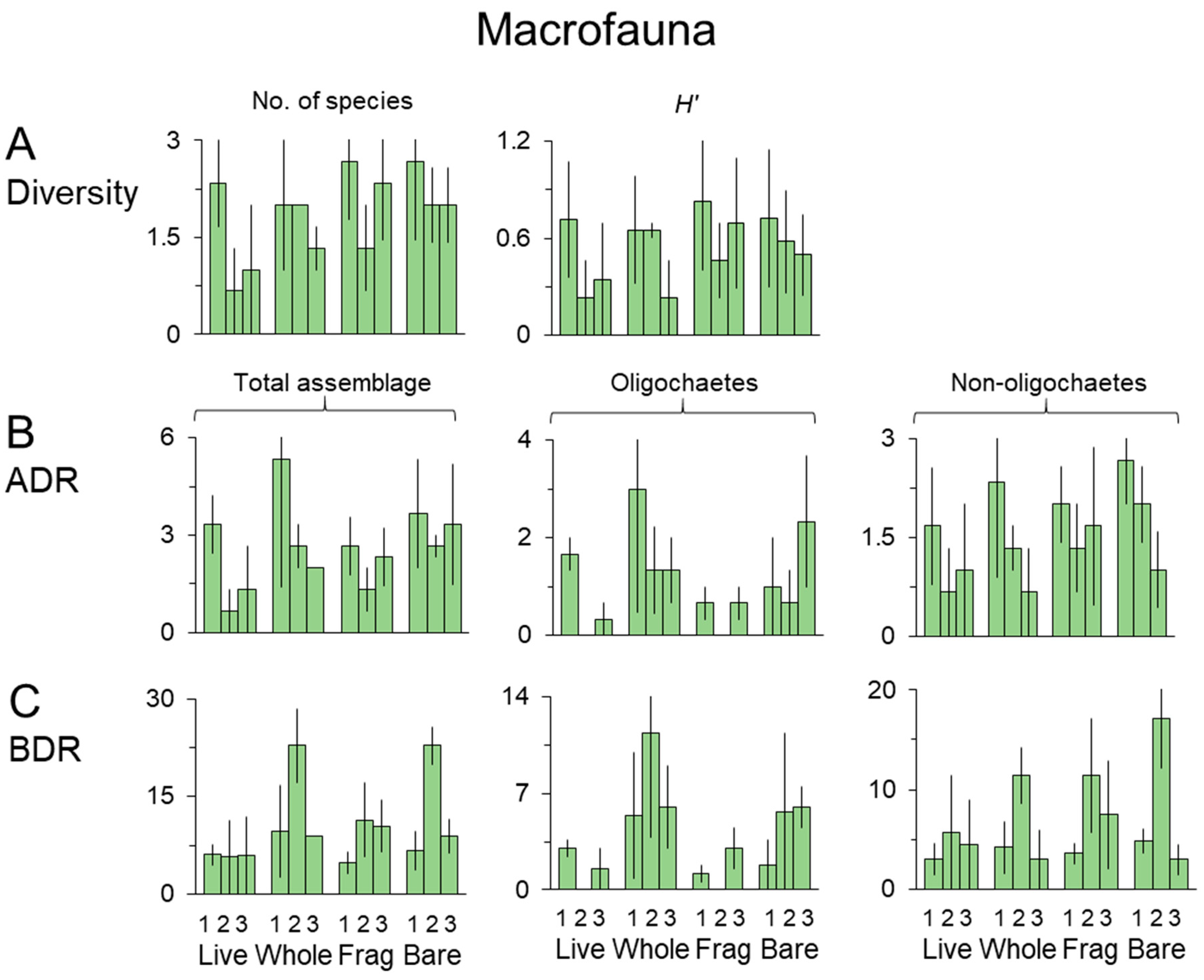
3.3. Macrofauna
4. Discussion
4.1. Cover Types
4.2. Days and Wind Condition
4.3. Modes of Dispersal, Mobility, and Turnover Times
4.4. Space and Time in Collapsed Mussel Beds
Supplementary Materials
Author Contributions
Funding
Acknowledgments
Conflicts of Interest
Appendix A

| Taxon | Rank | Mean | SE | |
|---|---|---|---|---|
| Meiofauna | ||||
| Copepoda | 1 | 268.94 | 39.57 | |
| Nematoda | 2 | 192.06 | 45.47 | |
| Foraminifera | 3 | 19.22 | 3.76 | |
| Ostracoda | 4 | 1.53 | 0.36 | |
| Kinorhyncha | 5 | 0.42 | 0.13 | |
| Halacaridae | 6 | 0.28 | 0.18 | |
| Cumacea | 7 | 0.08 | 0.06 | |
| Acarina | 8 | 0.03 | 0.03 | |
| Macrofauna | ||||
| Tubificoides benedeni | O | 1 | 1.08 | 0.27 |
| Lepidonotus squamatus | P | 2 | 0.42 | 0.14 |
| Polychaeta errant juvenile juvenile | P | 3 | 0.22 | 0.08 |
| Isopoda sp. A | A | 4 | 0.17 | 0.07 |
| Ampharetidae sp. A | P | 5 | 0.11 | 0.05 |
| Capitella capitata | P | 6 | 0.06 | 0.04 |
| Polycheata sp. A juvenile | P | 6 | 0.06 | 0.04 |
| Mya arenaria | M | 6 | 0.06 | 0.04 |
| Ampelisca abdita | A | 6 | 0.06 | 0.04 |
| Carcinus maenas | A | 6 | 0.06 | 0.04 |
| Gammaridae sp. A | A | 6 | 0.06 | 0.04 |
| Littorina littorea | M | 6 | 0.06 | 0.04 |
| Phyllodocidae sp. A | P | 6 | 0.06 | 0.04 |
| Lineus viridis | N | 14 | 0.03 | 0.03 |
| Hetermastus filiformis | P | 14 | 0.03 | 0.03 |
| Gammarus finmarchicus | A | 14 | 0.03 | 0.03 |
| Polycheata sp. B juvenile | P | 14 | 0.03 | 0.03 |
| Gammarus oceanicus | A | 14 | 0.03 | 0.03 |
| Polycheata sp. C juvenile | P | 14 | 0.03 | 0.03 |
References
- Commito, J.A. Adult larval interactions: Predictions, mussels, and cocoons. Estuar. Coast. Shelf Sci. 1987, 25, 599–606. [Google Scholar] [CrossRef]
- Commito, J.A.; Celano, E.A.; Celico, H.J.; Como, S.; Johnson, C.P. Mussels matter: Postlarval dispersal dynamics altered by a spatially complex ecosystem engineer. J. Exp. Mar. Biol. Ecol. 2005, 316, 133–147. [Google Scholar] [CrossRef]
- Commito, J.A.; Como, S.; Grupe, B.M.; Dow, W.E. Species diversity in the soft-bottom intertidal zone: Biogenic structure, sediment, and macrofauna across mussel bed spatial scales. J. Exp. Mar. Biol. Ecol. 2008, 366, 70–81. [Google Scholar] [CrossRef]
- Commito, J.A.; Jones, B.R.; Jones, M.A.; Winders, S.E.; Como, S. What happens after mussels die? Biogenic legacy effects on community structure and ecosystem processes. J. Exp. Mar. Biol. Ecol. 2018, 506, 30–41. [Google Scholar] [CrossRef]
- Thiel, M.; Ullrich, N. Hard rock versus soft bottom: The fauna associated with intertidal mussel beds on hard bottoms along the coast of Chile, and considerations on the functional role of mussel beds. Helgol. Mar. Res. 2002, 56, 21–30. [Google Scholar] [CrossRef]
- Norling, P.; Kautsky, N. Structural and functional effects of Mytilus edulis on diversity of associated species and ecosystem functioning. Mar. Ecol. Prog. Ser. 2007, 351, 163–175. [Google Scholar] [CrossRef]
- Norling, P.; Kautsky, N. Patches of the mussel Mytilus sp. are islands of high biodiversity in subtidal sediment habitats in the Baltic Sea. Aquat. Biol. 2008, 4, 75–87. [Google Scholar] [CrossRef]
- Bouma, T.J.; Olenin, S.; Reise, K.; Ysebaert, T. Ecosystem engineering and biodiversity in coastal sediments: Posing hypotheses. Helgol. Mar. Res. 2009, 63, 95–106. [Google Scholar] [CrossRef]
- Buschbaum, C.; Dittmann, S.; Hong, J.-H.; Hwang, I.-S.; Strasser, M.; Thiel, M.; Valdiva, N.; Yoon, S.-P.; Reise, K. Mytilid mussels: Global habitat engineers in coastal sediments. Helgol. Mar. Res. 2009, 63, 47–58. [Google Scholar] [CrossRef]
- Gutiérrez, J.L.; Jones, C.G.; Byers, J.E.; Arkema, K.K.; Berkenbusch, K.; Commito, J.A.; Duarte, C.M.; Hacker, S.D.; Lambrinos, J.G.; Hendriks, I.E.; et al. Physical ecosystem engineers and the functioning of estuaries and coasts. In Treatise on Estuarine and Coastal Science; Wolanski, E., McLusky, D.S., Eds.; Elsevier Academic Press: Waltham, MA, USA, 2011; Volume 7, pp. 53–81. ISBN 9780080878850. [Google Scholar]
- Nehls, G.; Thiel, M. Large-scale distribution patterns of the mussel Mytilus edulis in the Wadden Sea of Schleswig–Holstein: Do storms structure the ecosystem? Neth. J. Sea Res. 1993, 31, 181–187. [Google Scholar] [CrossRef]
- Reusch, T.B.H.; Chapman, A.R.O. Persistence and space occupancy by subtidal blue mussel patches. Ecol. Monogr. 1997, 67, 65–87. [Google Scholar] [CrossRef]
- Hertweck, G.; Liebezeit, G. Historic mussel beds (Mytilus edulis) in the sedimentary record of a back-barrier tidal flat near Spiekeroog Island, southern North Sea. Helgol. Mar. Res. 2002, 56, 51–58. [Google Scholar] [CrossRef]
- Folmer, E.O.; Drent, J.; Troost, K.; Büttger, H.; Dankers, N.; Jansen, J.; van Stralen, M.; Millat, G.; Herlyn, M.; Philippart, C.J. Large-scale spatial dynamics of intertidal mussel (Mytilus edulis L.) bed coverage in the German and Dutch Wadden Sea. Ecosystems 2014, 17, 550–566. [Google Scholar] [CrossRef]
- Khaitov, V.M.; Lentsman, N.V. The cycle of mussels: Long-term dynamics of mussel beds on intertidal soft bottoms at the White Sea. Hydrobiologia 2016, 781, 161–180. [Google Scholar] [CrossRef]
- Helmuth, B.; Mieszkowska, N.; Moore, P.; Hawkins, S.J. Living on the edge of two changing worlds: Forecasting the responses of rocky intertidal ecosystems to climate change. Ann. Rev. Ecol. Evol. Syst. 2006, 37, 373–404. [Google Scholar] [CrossRef]
- Jones, S.J.; Lima, F.P.; Wethey, D.S. Rising environmental temperatures and biogeography: Poleward range contraction of the blue mussel, Mytilus edulis L., in the western Atlantic. J Biogeogr. 2010, 37, 2243–2259. [Google Scholar] [CrossRef]
- Sorte, C.J.B.; Jones, S.J.; Miller, L.P. Geographic variation in temperature tolerance as an indicator of potential population responses to climate change. J. Exp. Mar. Biol. Ecol. 2011, 400, 209–217. [Google Scholar] [CrossRef]
- Sorte, C.J.B.; Davidson, V.E.; Franklin, M.C.; Benes, K.M.; Doellman, R.J.; Etter, R.J.; Hannigan, R.E.; Lubchenco, J.; Menge, B.A. Long-term declines in an intertidal foundation species parallel shifts in community composition. Glob. Chang. Biol. 2016. [Google Scholar] [CrossRef]
- Lesser, M.P. Climate change stressors cause metabolic depression in the blue mussel, Mytilus edulis, from the Gulf of Maine. Limnol. Oceanogr. 2016, 61, 1705–1717. [Google Scholar] [CrossRef]
- Steeves, L.E.; Filgueira, R.; Guyondet, T.; Chassé, J.; Comeau, L. Past, present, and future: Performance of two bivalve species under changing environmental conditions. Front. Mar. Sci. 2018, 5, 184. [Google Scholar] [CrossRef]
- Grosholz, E.D.; Ruiz, G.M. Predicting the impact of introduced marine species: Lessons from the multiple invasions of the European green crab Carcinus maenas. Biol. Conserv. 1996, 78, 59–66. [Google Scholar] [CrossRef]
- Whitlow, W.L.; Grabowski, J.H. Examining how landscapes influence benthic community assemblages in seagrass and mudflat habitats in southern Maine. J. Exp. Mar. Biol. Ecol. 2012, 411, 1–6. [Google Scholar] [CrossRef]
- Petraitis, P.S.; Dudgeon, S.R. Variation in recruitment and the establishment of alternative community states. Ecology 2015, 96, 3186–3196. [Google Scholar] [CrossRef] [PubMed]
- Tan, E.B.P.; Beal, B.F. Interactions between the invasive European green crab, Carcinus maenas (L.), and juveniles of the soft-shell clam, Mya arenaria L., in eastern Maine, USA. J. Exp. Mar. Biol. Ecol. 2015, 462, 62–73. [Google Scholar] [CrossRef]
- Commito, J.A.; Dow, W.E.; Grupe, B.M. Hierarchical spatial structure in soft-bottom mussel beds. J. Exp. Mar. Biol. Ecol. 2006, 330, 27–37. [Google Scholar] [CrossRef]
- Snover, M.L.; Commito, J.A. The fractal geometry of Mytilus edulis L. spatial distribution in a soft-bottom system. J. Exp. Mar. Biol. Ecol. 1998, 223, 53–64. [Google Scholar] [CrossRef]
- Commito, J.A.; Rusignuolo, B.R. Structural complexity in mussel beds: The fractal geometry of surface topography. J. Exp. Mar. Biol. Ecol. 2000, 225, 133–152. [Google Scholar] [CrossRef]
- Crawford, T.W.; Commito, J.A.; Borowik, A.M. Fractal characterization of Mytilus edulis L. spatial structure in intertidal landscapes using GIS methods. Landsc. Ecol. 2006, 21, 1033–1044. [Google Scholar] [CrossRef]
- Commito, J.A.; Commito, A.E.; Platt, R.V.; Grupe, B.M.; Piniak, W.E.D.; Gownaris, N.J.; Reeves, K.A.; Vissichelli, A.M. Recruitment facilitation and spatial pattern formation in soft-bottom mussel beds. Ecosphere 2014, 5, art160. [Google Scholar] [CrossRef]
- Commito, J.A.; Gownaris, N.J.; Haulsee, D.E.; Coleman, S.E.; Beal, B.F. Separation anxiety: Mussels self-organize into similar power-law clusters regardless of predation threat cues. Mar. Ecol. Prog. Ser. 2016, 547, 107–119. [Google Scholar] [CrossRef]
- Butman, C.A.; Fréchette, M.; Geyer, W.R.; Starczak, V.R. Flume experiments on food supply to the blue mussel Mytilus edulis L. as a function of boundary-layer flow. Limnol. Oceanogr. 1994, 39, 1755–1768. [Google Scholar] [CrossRef]
- Commito, J.A.; Dankers, N. Dynamics of spatial and temporal complexity in European and North American soft-bottom mussel beds. In Ecological Comparisons of Sedimentary Shores; Reise, K., Ed.; Springer: Heidelberg, Germany, 2001; pp. 39–59. ISBN 3-540-41254-9. [Google Scholar]
- Widdows, J.; Brinsley, M. Impact of biotic and abiotic processes on sediment dynamics and the consequences to the structure and functioning of the intertidal zone. J. Sea Res. 2002, 48, 143–156. [Google Scholar] [CrossRef]
- Widdows, J.; Pope, N.D.; Brinsley, M.D.; Gascoigne, J.; Kaiser, M.J. Influence of self-organised structures on near-bed hydrodynamics and sediment dynamics within a mussel (Mytilus edulis) bed in the Menai Strait. J. Exp. Mar. Biol. Ecol. 2009, 379, 92–100. [Google Scholar] [CrossRef]
- Gutiérrez, J.L.; Jones, C.G.; Strayer, D.L.; Iribarne, O.O. Mollusks as ecosystem engineers: The role of shell production in aquatic habitats. Oikos 2003, 101, 79–90. [Google Scholar] [CrossRef]
- Emerson, C.W.; Grant, J. The control of soft-shell clam (Mya arenaria) recruitment on intertidal sandflats by bedload sediment transport. Limnol. Oceanogr. 1991, 36, 1288–1300. [Google Scholar] [CrossRef]
- Armonies, W. Drifting meio-and microbenthic invertebrates on tidal flats in Königshafen: A review. Helgol. Meeresunters. 1994, 48, 299–320. [Google Scholar] [CrossRef]
- Commito, J.A.; Thrush, S.A.; Pridmore, R.D.; Hewitt, J.E.; Cummings, V.J. Dispersal dynamics in a wind-driven benthic system. Limnol. Oceanogr. 1995, 40, 1513–1518. [Google Scholar] [CrossRef] [Green Version]
- Turner, S.J.; Grant, J.; Pridmore, R.D.; Hewitt, J.E.; Wilkinson, M.R.; Hume, T.M.; Morrisey, D.J. Bedload and water-column transport and colonization processes by post-settlement benthic macrofauna: Does infaunal density matter? J. Exp. Mar. Biol. Ecol. 1997, 216, 51–75. [Google Scholar] [CrossRef]
- Lundquist, C.J.; Thrush, S.F.; Hewitt, J.E.; Halliday, J.; MacDonald, I.; Cummings, V.J. Spatial variability in recolonisation potential: Influence of organism behaviour and hydrodynamics on the distribution of macrofaunal colonists. Mar. Ecol. Prog. Ser. 2006, 324, 67–81. [Google Scholar] [CrossRef]
- Hunt, H.L.; Maltais, M.-J.; Fugate, D.C.; Chant, R.J. Spatial and temporal variability in juvenile bivalve dispersal: Effects of sediment transport and flow regime. Mar. Ecol. Prog. Ser. 2007, 352, 145–159. [Google Scholar] [CrossRef]
- Jennings, L.B.; Hunt, H.L. Distances of dispersal of juvenile bivalves (Mya arenaria (Linnaeus), Mercenaria mercenaria (Linnaeus), Gemma gemma (Totten)). J. Exp. Mar. Biol. Ecol. 2009, 376, 76–84. [Google Scholar] [CrossRef]
- Valanko, S.; Norkko, A.; Norkko, J. Rates of post-larval bedload dispersal in a non-tidal soft-sediment system. Mar. Ecol. Prog. Ser. 2010, 416, 145–163. [Google Scholar] [CrossRef] [Green Version]
- Valanko, S.; Norkko, A.; Norkko, J. Strategies of post-larval dispersal in non-tidal soft-sediment communities. J. Exp. Mar. Biol. Ecol. 2010, 384, 51–60. [Google Scholar] [CrossRef]
- Pacheco, A.S.; Uribe, R.A.; Thiel, M.; Oliva, M.E.; Riascos, J.M. Dispersal of post-larval macrobenthos in subtidal sedimentary habitats: Roles of vertical diel migration, water column, bedload transport and biological traits’ expression. J. Sea Res. 2013, 77, 79–92. [Google Scholar] [CrossRef]
- Green, M.O.; Coco, G. Review of wave-driven sediment resuspension and transport in estuaries. Rev. Geophys. 2014, 52, 77–117. [Google Scholar] [CrossRef] [Green Version]
- Levin, S.A.; Pacala, S.W. Theories of simplification and scaling of spatially distributed processes. In Spatial Ecology: The Role of Space in Population Dynamics and Interspecific Interactions; Tilman, D., Kareiva, P., Eds.; Princeton Univ. Press: Princeton, NJ, USA, 1997; pp. 271–295. ISBN 9780691016528. [Google Scholar]
- Hanski, I. Metapopulation Ecology; Oxford Univ. Press: Oxford, UK, 1999; ISBN 9780198540656. [Google Scholar]
- Hiebeler, D. Populations on fragmented landscapes with spatially structured heterogeneities: Landscape generation and local dispersal. Ecology 2000, 81, 1629–1641. [Google Scholar] [CrossRef]
- Thrush, S.F.; Hewitt, J.; Cummings, V.; Green, M.; Funnell, G.A.; Wilkinson, M.R. The generality of field experiments: Interactions between local and broad-scale processes. Ecology 2000, 81, 399–415. [Google Scholar] [CrossRef]
- Pilditch, C.A.; Valanko, S.; Norkko, J.; Norkko, A. Post-settlement dispersal: The neglected link in maintenance of soft-sediment biodiversity. Biol. Lett. 2015, 11, 20140795. [Google Scholar] [CrossRef]
- Palmer, M.A. Dispersal of marine meiofauna: A review and conceptual model explaining passive transport and active emergence with implications for recruitment. Mar. Ecol. Prog. Ser. 1988, 48, 81–91. [Google Scholar] [CrossRef]
- Fegley, S.R. A comparison of meiofaunal settlement onto the sediment surface and recolonization of defaunated sandy sediment. J. Exp. Mar. Biol. Ecol. 1988, 123, 97–113. [Google Scholar] [CrossRef]
- DePatra, K.D.; Levin, L.A. Evidence of the passive deposition of meiofauna into fiddler crab burrows. J. Exp. Mar. Biol. Ecol. 1989, 125, 173–192. [Google Scholar] [CrossRef]
- Fleeger, J.W.; Yund, P.O.; Sun, B. Active and passive processes associated with initial settlement and postsettlement dispersal of suspended meiobenthic copepods. J. Mar. Res. 1995, 53, 609–645. [Google Scholar] [CrossRef]
- Commito, J.A.; Tita, G. Differential dispersal rates in an intertidal meiofauna assemblage. J. Exp. Mar. Biol. Ecol. 2002, 268, 237–256. [Google Scholar] [CrossRef]
- Hunt, H.L. Effects of sediment source and flow regime on clam and sediment transport. Mar. Ecol. Prog. Ser. 2005, 296, 143–153. [Google Scholar] [CrossRef] [Green Version]
- Hurlbert, S.H. Pseudoreplication and the design of ecological field experiments. Ecol. Monogr. 1984, 54, 187–211. [Google Scholar] [CrossRef]
- Pollock, L.W. A Practical Guide to the Marine Animals of Northeastern North America; Rutgers University Press: New Brunswick, NJ, USA, 1998; ISBN 0-8135-2398-2. [Google Scholar]
- Dean, W.E. Determination of carbonate and organic matter in calcareous sediments and sedimentary rocks by loss on ignition: A comparison with other methods. J. Sediment. Petrol. 1974, 44, 242–248. [Google Scholar]
- Commito, J.A.; Currier, C.A.; Kane, L.R.; Reinsel, K.A.; Ulm, I.M. Dispersal dynamics of the bivalve Gemma gemma in a patchy environment. Ecol. Monogr. 1995, 65, 1–20. [Google Scholar] [CrossRef]
- Underwood, A.J. Experiments in Ecology: Their Logical Design and Interpretation Using Analysis of Variance; Cambridge University: Cambridge, UK, 1997; ISBN 0-521-55329-6. [Google Scholar]
- StatSoft 6.1. STATISTICA Data Analysis Software System; StatSoft, Inc.: Tulsa, OK, USA, 1994. [Google Scholar]
- Anderson, M.J. A new method for non-parametric multivariate analysis of variance. Aust. J. Ecol. 2001, 26, 32–46. [Google Scholar]
- McArdle, B.H.; Anderson, M.J. Fitting multivariate models to community data: A comment on distance-based redundancy analysis. Ecology 2001, 82, 290–297. [Google Scholar] [CrossRef]
- R Core Development Team. R: A Language and Environment for Statistical Computing 2017; R Foundation for Statistical Computing: Vienna, Austria, 2015; Available online: http://www.R-project.org/ (accessed on 12 June 2015).
- Clarke, K.R.; Warwick, R.M. Changes in Marine Communities: An Approach to Statistical Analysis and Interpretation, 2nd ed.; PRIMER-E: Plymouth, UK, 2001. [Google Scholar]
- Zar, J.H. Biostatistical Analysis, 4th ed.; Prentice Hall: Upper Saddle River, NJ, USA, 1999; ISBN 0-13-081542-X. [Google Scholar]
- Hily, C. Is the activity of benthic suspension feeders a factor controlling water quality in the Bay of Brest? Mar. Ecol. Prog. Ser. 1991, 69, 179–188. [Google Scholar] [CrossRef]
- Kraeuter, J.N.; Kennish, M.J.; Dobarro, J.; Fegley, S.R.; Flimlin, G.E. Rehabilitation of the northern quahog (hard clam) (Mercenaria mercenaria) habitats by shelling—11 years in Barnegat Bay, New Jersey. J. Shellfish Res. 2003, 22, 61–67. [Google Scholar]
- Guay, M.; Himmelman, J.H. Would adding scallop shells (Chlamys islandica) to the sea bottom enhance recruitment of commercial species? J. Exp. Mar. Biol. Ecol. 2004, 312, 299–317. [Google Scholar] [CrossRef]
- Ribeiro, P.D.; Iribarne, O.O.; Daleo, P. The relative importance of substratum characteristics and recruitment in determining the spatial distribution of the fiddler crab Uca uruguayensis Nobili. J. Exp. Mar. Biol. Ecol. 2005, 314, 99–111. [Google Scholar] [CrossRef]
- Rodney, W.S.; Paynter, K.T. Comparisons of macrofaunal assemblages on restored and non-restored oyster reefs in mesohaline regions of Chesapeake Bay in Maryland. J. Exp. Mar. Biol. Ecol. 2006, 35, 39–51. [Google Scholar] [CrossRef]
- Summerhayes, S.A.; Bishop, M.J.; Leigh, A.; Kelaher, B.P. Effects of oyster death and shell disarticulation on associated communities of epibiota. J. Exp. Mar. Biol. Ecol. 2009, 379, 60–67. [Google Scholar] [CrossRef]
- Wilding, T.A.; Nickell, T.D. Changes in benthos associated with mussel (Mytilus edulis L.) farms on the West-Coast of Scotland. PLoS ONE 2013, 8, e68313. [Google Scholar] [CrossRef] [PubMed]
- Hubbard, W.A. Benthic studies in upper Buzzards Bay, Massachusetts: 2011–12 as compared to 1955. Mar. Ecol. 2016, 37, 532–542. [Google Scholar] [CrossRef]
- Tomatsuri, M.; Kon, K. Effects of dead oyster shells as a habitat for the benthic faunal community along rocky shore regions. Hydrobiologia 2017, 790, 25–232. [Google Scholar] [CrossRef]
- Gutiérrez, J.L.; Iribarne, O.O. Role of Holocene beds of the stout razor clam Tagelus plebeius in structuring present benthic communities. Mar. Ecol. Prog. Ser. 1999, 185, 213–228. [Google Scholar] [CrossRef]
- Bomkamp, R.E.; Page, H.M.; Dugan, J.E. Role of food subsidies and habitat structure in influencing benthic communities of shell mounds at sites of existing and former offshore oil platforms. Mar. Biol. 2004, 146, 201–211. [Google Scholar] [CrossRef]
- Hewitt, J.E.; Thrush, S.F.; Halliday, J.; Duffy, C. The importance of small-scale habitat structure for maintaining beta diversity. Ecology 2005, 86, 1619–1626. [Google Scholar] [CrossRef]
- Nicastro, A.; Bishop, M.; Kelaher, B.P.; Benedetti-Cecchi, L. Export of non-native gastropod shells to a coastal lagoon: Alteration of habitat structure has negligible effects on infauna. J. Exp. Mar. Biol. Ecol. 2009, 374, 31–36. [Google Scholar] [CrossRef]
- Mann, R.; Southworth, M.; Fisher, R.J.; Wesson, J.A.; Erskine, A.J.; Leggett, T. Oyster planting protocols to deter losses to cownose ray predation. J. Shellfish Res. 2016, 35, 127–136. [Google Scholar] [CrossRef]
- Folkard, A.M.; Gascoigne, J. Hydrodynamics of discontinuous mussel beds: Laboratory flume simulations. J. Sea Res. 2009, 62, 250–257. [Google Scholar] [CrossRef]
- wa Kangeri, A.K.; Jansen, J.M.; Joppe, D.J.; Dankers, N.M.J.A. In situ investigation of the effects of current velocity on sedimentary mussel bed stability. J. Exp. Mar. Biol. Ecol. 2016, 485, 65–72. [Google Scholar] [CrossRef]
- Singer, J.K.; Anderson, J.B. Use of total grain-size distributions to define bed erosion and transport for poorly sorted sediment undergoing simulated bioturbation. Mar. Geol. 1984, 57, 335–359. [Google Scholar] [CrossRef]
- Chen, P.; Fu, Z.; Lim, A.; Rodrigues, B. Two-Dimensional Packing for Irregular Shaped Objects. In Proceedings of the 36th Hawaii International Conference on System Sciences, Big Island, HI, USA, USA, 6–9 January 2003; Institute of Electrical and Electronics Engineers: New York, NY, USA, 2003. [Google Scholar] [CrossRef]
- Ragnarsson, S.A.; Raffaelli, D. Effects of Mytilus edulis L. on the invertebrate fauna of sediments. J. Exp. Mar. Biol. Ecol. 1999, 241, 31–43. [Google Scholar] [CrossRef]
- Albrecht, A.; Reise, K. Effects of Fucus vesiculosus covering intertidal mussel beds in the Wadden Sea. Helgol. Meeresunters. 1994, 48, 243–256. [Google Scholar] [CrossRef]
- Albrecht, S.H. Soft bottom versus hard rock: Community ecology of macroalgae on intertidal mussel beds in the Wadden Sea. J. Exp. Mar. Biol. Ecol. 1998, 229, 85–109. [Google Scholar] [CrossRef]
- Crooks, J.A. Habitat alteration and community-level effects of an exotic mussel, Musculista senhousia. Mar. Ecol. Prog. Ser. 1998, 162, 137–152. [Google Scholar] [CrossRef]
- Crooks, J.A.; Khim, H.S. Architectural vs. biological effects of a habitat-altering, exotic mussel, Musculista senhousia. J. Exp. Mar. Biol. Ecol. 1999, 240, 53–75. [Google Scholar] [CrossRef]
- Norkko, A.; Hewitt, J.E.; Thrush, S.F.; Funnell, G.A. Benthic–pelagic coupling and suspension-feeding bivalves: Linking site-specific sediment flux and biodeposition to benthic community structure. Limnol. Oceanogr. 2001, 46, 2067–2072. [Google Scholar] [CrossRef]
- Hewitt, J.E.; Thrush, S.F.; Legendre, P.; Cummings, V.J.; Norkko, A. Integrating heterogeneity across spatial scales: Interactions between Atrina zelandica and benthic macrofauna. Mar. Ecol. Prog. Ser. 2002, 239, 115–128. [Google Scholar] [CrossRef]
- Donadi, S.; van der Heide, T.; van der Zee, E.M.; Eklöf, J.S.; van de Koppel, J.; Weerman, E.J.; Piersma, T.; Olff, H.; Eriksson, B.K. Cross-habitat interactions among bivalve species control community structure on intertidal flats. Ecology 2013, 94, 489–498. [Google Scholar] [CrossRef] [PubMed] [Green Version]
- Sun, B.; Fleeger, J.W. Field experiments on the colonization of meiofauna into sediment depressions. Mar. Ecol. Prog. Ser. 1994, 110, 167–175. [Google Scholar] [CrossRef]
- Zühlke, R.; Reise, K. Response of macrofauna to drifting tidal sediments. Helgol. Meeresunters. 1994, 48, 277–289. [Google Scholar] [CrossRef] [Green Version]
- Pershing, A.J.; Alexander, M.A.; Hernandez, C.M.; Kerr, L.A.; Le Bris, A.; Mills, K.E.; Nye, J.A.; Record, N.R.; Scannell, H.A.; Scott, J.D.; et al. Slow adaptation in the face of rapid warming leads to collapse of the Gulf of Maine cod fishery. Science 2015, 350, 809–812. [Google Scholar] [CrossRef]
- Sallenger, A.H.; Doran, K.S.; Howd, P.A. Hotspot of accelerated sea-level rise on the Atlantic coast of North America. Nat. Clim. Chang. 2012, 2, 884–888. [Google Scholar] [CrossRef] [Green Version]
- Donnelly, J.P.; Bertness, M.D. Rapid shoreward encroachment of salt marsh cordgrass in response to accelerated sea-level rise. Proc. Natl. Acad. Sci. USA 2001, 98, 14218–14223. [Google Scholar] [CrossRef] [Green Version]
- van der Wegen, M.; Jaffe, B.; Foxgrover, A.; Roelvink, D. Mudflat morphodynamics and the impact of sea level rise in south San Francisco Bay. Estuar. Coasts 2017, 40, 37–49. [Google Scholar] [CrossRef]
- Beaugrand, G.; Edwards, M.; Brander, K.; Luczak, C.; Ibanez, F. Causes and projections of abrupt climate–driven ecosystem shifts in the North Atlantic. Ecol. Lett. 2008, 11, 157–1168. [Google Scholar] [CrossRef]
- Edwards, M.; Beaugrand, G.; Helaouët, P.; Alheit, J.; Coombs, S. Marine ecosystem response to the Atlantic multidecadal oscillation. PLoS ONE 2013, 8, e57212. [Google Scholar] [CrossRef]
- Greene, C.H.; Meyer-Gutbrod, E.; Monger, B.C.; McGarry, L.P.; Pershing, A.J.; Belkin, I.M.; Fratantoni, P.S.; Mountain, D.G.; Pickart, R.S.; Proshutinsky, A.; et al. Remote climate forcing of decadal-scale regime shifts in Northwest Atlantic shelf ecosystems. Limnol. Oceanogr. 2013, 58, 803–816. [Google Scholar] [CrossRef] [Green Version]
- Reise, K.; Buschbaum, C.; Büttger, H.; Wegner, K.M. Invading oysters and native mussels: From hostile takeover to compatible bedfellows. Ecosphere 2017, 8, e01949. [Google Scholar] [CrossRef]
- Kidwell, S.M.; Jablonski, D. Taphonomic feedback: Ecological consequences of shell accumulation. In Biotic Interactions in Recent and Fossil Benthic Communities; Tevesz, M.J.S., McCall, P.L., Eds.; Plenum Press: New York, New York, USA, 1983; pp. 195–248. ISBN 978-1-4757-0742-7. [Google Scholar]
- Reise, K. Sediment mediated species interactions in coastal waters. J. Sea Res. 2002, 48, 127–141. [Google Scholar] [CrossRef]
- Powell, E.N.; Staff, G.M.; Callender, W.R.; Ashton-Alcox, K.A.; Brett, C.E.; Parsons-Hubbard, K.M.; Walker, S.E.; Raymond, A. Taphonomic degradation of molluscan remains during thirteen years on the continental shelf and slope of the northwestern Gulf of Mexico. Palaeogeogr. Palaeoclimatol. Palaeoecol. 2011, 312, 209–232. [Google Scholar] [CrossRef]


| Sediment | |||||||
|---|---|---|---|---|---|---|---|
| Coarse (g) | Fine (g) | Silt-Clay (g) | |||||
| Source | DF | F | P | F | P | F | P |
| Day | 2 | 2.18 | 0.194 | 7.13 | 0.026 | 2.47 | 0.165 |
| Cover | 3 | 2.05 | 0.134 | 0.70 | 0.560 | 5.26 | 0.006 |
| Day × Cover | 6 | 0.70 | 0.652 | 0.92 | 0.500 | 1.35 | 0.275 |
| Residual | 24 | ||||||
| Total | 35 | ||||||
| Transformation | Ln(x + 1) | Ln(x + 1) | |||||
| SNK Day | D1 > D2 = D3 | ||||||
| SNK Cover | NAH (L > F) | ||||||
| Total (g) | Organic Matter (%) | ||||||
| Source | DF | F | P | F | P | ||
| Day | 2 | 7.01 | 0.027 | 11.34 | 0.0003 | ||
| Cover | 3 | 1.21 | 0.328 | 0.51 | 0.680 | ||
| Day × Cover | 6 | 0.68 | 0.664 | 1.02 | 0.438 | ||
| Residual | 24 | ||||||
| Total | 35 | ||||||
| Transformation | Ln(x + 1) | Ln(x + 1) | |||||
| SNK Day | D1 > D3 = D2 | D3 > D1 > D2 | |||||
| SNK Cover | |||||||
| Meiofauna | |||||||
|---|---|---|---|---|---|---|---|
| No. of Taxa | H’ | Total Assemblage | |||||
| Source | DF | F | P | F | P | F | P |
| Day | 2 | 0.72 | 0.495 | 4.17 | 0.028 | 6.36 | 0.006 |
| Cover | 3 | 1.20 | 0.333 | 5.70 | 0.004 | 4.34 | 0.014 |
| Day × Cover | 6 | 0.54 | 0.772 | 2.32 | 0.066 | 0.29 | 0.936 |
| Residual | 24 | ||||||
| Total | 35 | ||||||
| Transformation | Ln(x + 1) | ||||||
| SNK Day | D1 > D2 = D3 | D1 = D3 > D2 | |||||
| SNK Cover | NAH (B > L) | W = L = B > F | |||||
| Copepods | Nematodes | Foraminiferans | |||||
| Source | DF | F | P | F | P | F | P |
| Day | 2 | 3.72 | 0.039 | 10.99 | 0.0004 | 3.57 | 0.044 |
| Cover | 3 | 3.67 | 0.026 | 4.04 | 0.019 | 4.39 | 0.013 |
| Day × Cover | 6 | 0.52 | 0.787 | 0.38 | 0.886 | 1.47 | 0.229 |
| Residual | 24 | ||||||
| Total | 35 | ||||||
| Transformation | Ln(x + 1) | Ln(x + 1) | Ln(x + 1) | ||||
| SNK Day | D1 = D3 > D2 | D1 > D3 = D2 | NAH (D1 > D3) | ||||
| SNK Cover | W = L = B > F | NAH (W > F) | NAH (B > F) | ||||
| Meiofauna | Macrofauna | ||||
|---|---|---|---|---|---|
| Source | DF | F | P | F | P |
| Day | 2 | 3.69 | 0.006 | 1.34 | 0.179 |
| Cover | 3 | 3.03 | 0.011 | 1.35 | 0.153 |
| Day × Cover | 6 | 0.56 | 0.934 | 1.41 | 0.076 |
| Residual | 24 | ||||
| Total | 35 | ||||
| Within Days: | |||||
| D1 | 40.41 | ||||
| D2 | 48.92 | ||||
| D3 | 41.65 | ||||
| Among Days: | |||||
| D1 vs. D2 | 53.39 | ||||
| D1 vs. D3 | 43.87 | ||||
| D2 vs. D3 | 47.84 | ||||
| Within Cover Types: | |||||
| L | 45.32 | ||||
| W | 47.15 | ||||
| F | 49.51 | ||||
| B | 30.04 | ||||
| Among Cover Types: | |||||
| B vs. L | 38.69 | ||||
| B vs. W | 43.06 | ||||
| B vs. F | 52.83 | ||||
| L vs. W | 48.8 | ||||
| L vs. F | 56.21 | ||||
| W vs. F | 48.66 | ||||
| Meiofauna | |||||
|---|---|---|---|---|---|
| Total Assemblage | Copepods | ||||
| Source | DF | F | P | F | P |
| Day | 2 | 2.32 | 0.120 | 1.40 | 0.267 |
| Cover | 3 | 5.21 | 0.007 | 3.29 | 0.038 |
| Day × Cover | 6 | 1.02 | 0.437 | 0.96 | 0.474 |
| Residual | 24 | ||||
| Total | 35 | ||||
| Transformation | Ln(x + 1) | Ln(x + 1) | |||
| SNK Day | |||||
| SNK Cover | W > L = F = B | W > F = L = B | |||
| Nematodes | Foraminiferans | ||||
| Source | DF | F | P | F | P |
| Day | 2 | 1.75 | 0.196 | 4.06 | 0.030 |
| Cover | 3 | 3.00 | 0.051 | 3.87 | 0.022 |
| Day × Cover | 6 | 0.57 | 0.752 | 0.89 | 0.521 |
| Residual | 24 | ||||
| Total | 35 | ||||
| Transformation | |||||
| SNK Day | D1 > D3 = D2 | ||||
| SNK Cover | NAH (W > F) | ||||
| Meiofauna | |||||
|---|---|---|---|---|---|
| Total Assemblage | Copepods | ||||
| Source | DF | F | P | F | P |
| Day | 2 | 0.98 | 0.389 | 3.77 | 0.038 |
| Cover | 3 | 2.22 | 0.112 | 2.20 | 0.114 |
| Day × Cover | 6 | 0.59 | 0.734 | 0.81 | 0.571 |
| Residual | 24 | ||||
| Total | 35 | ||||
| Transformation | |||||
| SNK Day | D2 = D3 > D1 | ||||
| SNK Cover | |||||
| Nematodes | Foraminiferans | ||||
| Source | DF | F | P | F | P |
| Day | 2 | 0.62 | 0.544 | 0.92 | 0.412 |
| Cover | 3 | 3.61 | 0.028 | 1.40 | 0.268 |
| Day × Cover | 6 | 0.29 | 0.938 | 1.02 | 0.438 |
| Residual | 24 | ||||
| Total | 35 | ||||
| Transformation | Ln(x + 1) | Ln(x + 1) | |||
| SNK Day | |||||
| SNK Cover | NAH (B > F) | ||||
| Macrofauna | |||||||
|---|---|---|---|---|---|---|---|
| No. of Species | H’ | Total Assemblage | |||||
| Source | DF | F | P | F | P | F | P |
| Day | 2 | 1.61 | 0.221 | 0.98 | 0.391 | 1.57 | 0.229 |
| Cover | 3 | 0.81 | 0.502 | 0.30 | 0.825 | 1.34 | 0.284 |
| Day × Cover | 6 | 0.34 | 0.910 | 0.24 | 0.958 | 0.49 | 0.809 |
| Residual | 24 | ||||||
| Total | 35 | ||||||
| Transformation | Ln(x + 1) | ||||||
| Oligochaetes | Non-Oligochaetes | ||||||
| Source | DF | F | P | F | P | ||
| Day | 2 | 1.96 | 0.163 | 1.88 | 0.175 | ||
| Cover | 3 | 1.29 | 0.302 | 0.48 | 0.698 | ||
| Day × Cover | 6 | 0.76 | 0.605 | 0.24 | 0.959 | ||
| Residual | 24 | ||||||
| Total | 35 | ||||||
| Transformation | Ln(x + 1) | ||||||
| Macrofauna Parameter | |||||||
|---|---|---|---|---|---|---|---|
| N | Oligochaetes | Non-Oligochaetes | |||||
| Source | DF | F | P | F | P | F | P |
| Day | 2 | 4.65 | 0.020 | 0.94 | 0.405 | 4.91 | 0.016 |
| Cover | 3 | 2.09 | 0.128 | 1.68 | 0.197 | 0.62 | 0.612 |
| Day × Cover | 6 | 1.08 | 0.403 | 0.91 | 0.502 | 0.64 | 0.699 |
| Residual | 24 | ||||||
| Total | 35 | ||||||
| Transformation | Ln(x + 1) | ||||||
| SNK Day | D2 > D3 = D1 | D2 > D3 = D1 | |||||
© 2019 by the authors. Licensee MDPI, Basel, Switzerland. This article is an open access article distributed under the terms and conditions of the Creative Commons Attribution (CC BY) license (http://creativecommons.org/licenses/by/4.0/).
Share and Cite
Commito, J.A.; Jones, B.R.; Jones, M.A.; Winders, S.E.; Como, S. After the Fall: Legacy Effects of Biogenic Structure on Wind-Generated Ecosystem Processes Following Mussel Bed Collapse. Diversity 2019, 11, 11. https://doi.org/10.3390/d11010011
Commito JA, Jones BR, Jones MA, Winders SE, Como S. After the Fall: Legacy Effects of Biogenic Structure on Wind-Generated Ecosystem Processes Following Mussel Bed Collapse. Diversity. 2019; 11(1):11. https://doi.org/10.3390/d11010011
Chicago/Turabian StyleCommito, John A., Brittany R. Jones, Mitchell A. Jones, Sondra E. Winders, and Serena Como. 2019. "After the Fall: Legacy Effects of Biogenic Structure on Wind-Generated Ecosystem Processes Following Mussel Bed Collapse" Diversity 11, no. 1: 11. https://doi.org/10.3390/d11010011
APA StyleCommito, J. A., Jones, B. R., Jones, M. A., Winders, S. E., & Como, S. (2019). After the Fall: Legacy Effects of Biogenic Structure on Wind-Generated Ecosystem Processes Following Mussel Bed Collapse. Diversity, 11(1), 11. https://doi.org/10.3390/d11010011