Article

Testing Hypotheses of Diversification in Panamanian Frogs and Freshwater Fishes Using Hierarchical Approximate Bayesian Computation with Model Averaging

by
Justin C. Bagley
1,2,*,
Michael J. Hickerson
3,4,5 and
Jerald B. Johnson
6,7
1
Department of Biology, Virginia Commonwealth University, Richmond, VA 23284, USA
2
Departamento de Zoologia, Instituto de Ciências Biológicas, Universidade de Brasília, Brasília 70910-900, Brazil
3
Biology Department, City College of New York, New York, NY 10031, USA
4
The Graduate Center, City University of New York, New York, NY 10016, USA
5
Division of Invertebrate Zoology, The American Museum of Natural History, New York, NY 10024, USA
6
Department of Biology, Brigham Young University, Provo, UT 84602, USA
7
Monte L. Bean Life Science Museum, Brigham Young University, Provo, UT 84602, USA
*
Author to whom correspondence should be addressed.
Diversity 2018, 10(4), 120; https://doi.org/10.3390/d10040120
Submission received: 9 September 2018 / Revised: 29 October 2018 / Accepted: 30 October 2018 / Published: 2 November 2018

Abstract

:
Most Neotropical frog and freshwater fish species sampled to date show phylogeographic breaks along the Pacific coast of the Isthmus of Panama, with lineages in Costa Rica and western Panama isolated from central Panama. We examine temporal patterns of diversification of taxa across this ‘western Panama isthmus’ (WPI) break to test hypotheses about the origin of species geographical distributions and genetic structuring in this region. We tested for synchronous diversification of four codistributed frog taxon-pairs and three fish taxon-pairs sharing the WPI break using hierarchical approximate Bayesian computation with model averaging based on mitochondrial DNA sequences. We also estimated lineage divergence times using full-Bayesian models. Several of our results supported synchronous divergences within the frog and freshwater fish assemblages; however, Bayes factor support was equivocal for or against synchronous or asynchronous diversification. Nevertheless, we infer that frog populations were likely isolated by one or multiple Pliocene–Pleistocene events more recently than predicted by previous models, while fish genetic diversity was structured by Pleistocene events. By integrating our results with external information from geology and elevational sea level modeling, we discuss the implications of our findings for understanding the biogeographical scenario of the diversification of Panamanian frogs and fishes. Consistent with the ‘Bermingham/Martin model’ (Molecular Ecology 1998, 7, 499–517), we conclude that the regional fish assemblage was fractured by processes shaping isthmian landscapes during the Pleistocene glaciations, including drainage basin isolation during lowered sea levels.

1. Introduction

By revealing the geographical histories of genetic lineages within species, phylogeography helps identify processes that influence the divergence, spread, and spatial-demographic fluctuations of lineages [1,2,3]. Single-species phylogeography surveys often reveal cryptic refugia and speciation events, for example [2,4,5]. By contrast, ‘comparative phylogeography’ presents a stronger approach for testing the generality of evolutionary patterns recovered within single species, often uncovering historical processes shaping species richness and genetic diversity [6,7]. Comparative phylogeography infers the histories of regional assemblages by testing for spatial and temporal phylogeographic congruence across codistributed species [1,8,9]. Congruent spatiotemporal divergences across taxa can indicate a shared history of responses to historical events [9,10].
Most comparative surveys in phylogeography are based on mitochondrial DNA (mtDNA) and are consequently subject to the caveats of using a single locus. Phylogeographic histories within individual species may be confounded by effects of stochastic variance in coalescent and mutational processes, natural selection, sex-biased dispersal, or reproductive success on genetic data [11,12,13,14,15]. Comparative studies guard against effects of such stochastic processes on inferences by searching for phylogeographic patterns replicated across multiple lineages [2,16]. This is analogous to improving evolutionary inferences through using multiple loci to estimate population parameters, multilocus models, or population/species trees across multiple gene genealogies [12,17,18]. Still, comparative approaches face major challenges to distinguish among potential scenarios that may have led to the observed patterns. Parameter estimates from mtDNA can suffer from low resolution, yielding wide confidence intervals that limit hypotheses testing [12]. The critical task of understanding the temporal framework of diversification to infer the historical biogeographical scenario underpinning spatial-genetic patterns can also be problematic, even if spatially congruent breaks are identified. Because variance in past effective population sizes (Ne), mutation rate, and generation time create high variation in gene tree topologies and their depths (correlated with timing of their divergences; e.g., [11,19]), what appear as multiple divergence events may actually reflect the obscured signal of a single event [20]. Thus, comparing independent gene-tree depths and divergence time estimates can lead to erroneous inferences of multiple vicariance events.
To guard against potential misinterpretations of biogeographical history, it is imperative to rigorously evaluate the timing of population divergences across species. Approximate Bayesian computation (ABC) methods for phylogeography allow accounting for potentially confounding stochastic coalescent effects while estimating parameters of phylogeographic datasets in such a way that sidesteps the need to calculate explicit likelihood functions. These “likelihood-free” methods permit simultaneously estimating demographic parameters and divergence times across populations by replacing the data with summary statistics, resulting in more efficient extraction of information, for example [21,22]. One broadly validated ABC method for comparative phylogeography, the MTML-msBayes (multi-taxa multi-locus msBayes) pipeline [22,23,24,25], permits comparing hypotheses in a parameter-rich hierarchical ABC (hABC) model using data from multiple codistributed population-pairs. This method has become widely used for testing explicit hypotheses about the timing of genetic divergences that have arisen during the assembly and diversification of regional species assemblages [26,27,28,29,30,31]. Based on simulations, some have cautioned that overly broad priors can result in low power to detect multiple divergences using MTML-msBayes [32]. However, this pitfall can be avoided by graphical sampling checks as well as comparing multiple MTML-msBayes model classes (priors) using ABC model averaging to account for uncertainty in model selection [24,33]). Other workers have also advocated leaving the summary statistics vector unsorted, as well as employing a Dirichlet-process prior as the hyperprior for the hyperparameter on the number of co-divergence events (Ψ) in the MTML-msBayes model and relying on this hyperparameter for inference [34,35,36]. However, our recent study using a cross-validation approach applied to simulated and empirical data, including the Panamanian datasets analyzed in the current paper, shows conclusively that choice of prior on Ψ has limited impact on inference, while re-sorting of summary statistics yields considerably more reliable results [37].
The Central American Isthmus has been an active area of phylogeographic research for nearly 20 years, with most studies focusing on inferring how, when, and why lineages colonized the isthmian landscape, diversified, and assembled into local communities [5]. A growing catalogue of species is being identified with common phylogeographic divergences across the Pacific-coastal lowlands of the Isthmus of Panama, with lineages in Costa Rica’s Golfo Dulce region and western Panama isolated from lineages in central Panama (Figure 1 and Figure 2; reviewed by [5]). This pattern has become known as the ‘western Panama isthmus’ (WPI) break [5]. Biogeographers interpret WPI breaks in frogs as resulting from multiple dispersals of different lineages into Central America across a continuous Miocene–Pliocene wet forest corridor, from both the north and the south [38,39,40,41], followed by vicariance caused by the development of tropical dry forest 12–4 million years ago (Ma; ‘dry forest hypothesis’; [42,43]). While frog fossils from the region are lacking, this scenario is supported by plant microfossils showing that modern dry forest species began appearing in central Panama up to mid-Pliocene [44,45]. Among freshwater fishes, the WPI break appears to reflect the effectiveness of rugged terrains at Soná and Azuero peninsulas (Figure 1) as biogeographical barriers to fish lineages, which arrived in multiple northwestward waves from South America since the Neogene. Bermingham and Martin [9] hypothesized that a corridor, formed by low sea level and tectonic uplift of the isthmus as the Cocos Ridge collided with the Panama microplate by ~7 Ma [46], permitted ‘early’ emplacement of freshwater fish species since Miocene–Pliocene. Subsequently, they argued that high eustatic sea levels of the mid-late Pliocene ~3.5–3 Ma [47] recreated a seaway over the isthmus, causing freshwater fishes to go extinct in central Panama ~3 Ma, before final isthmus emergence [9]. They hypothesized that the WPI break in fishes resulted from fragmentation due to drainage basin isolation during Pleistocene glacial periods over 2–0 Ma [9]. This ‘Bermingham/Martin model’ has also been invoked to explain phylogeographic patterns in pseudoscorpions, eels, catfishes, frogs, and other taxa, for example [5,48,49,50,51].
Clearly, previous studies generated or tested biogeographical models that provide convincing evidence for the WPI break. However, none of these studies explicitly accounted for genetic variance associated with coalescent processes, or among-lineage differences in demography or mutational rates, that may have influenced the variable patterns of genetic divergences of taxa associated with the WPI break ([9,42]; see Results). Thus, the temporal pattern and underlying mechanisms of diversification across the WPI break have not yet been fully explored. Additional studies are needed to evaluate whether the pattern of genetic structuring shared among frogs and freshwater fishes in the western Panama isthmus arose synchronously or asynchronously, and to determine the timing of historical events that have shaped community assembly and genetic divergence in this region.
The goal of this study is to examine the temporal patterns of diversification of frogs and freshwater fishes across the WPI break to test existing hypotheses about the origin of species distributions and genetic structuring in west-Pacific Panama. We use hABC simulations with ABC model averaging, and full-Bayesian divergence time estimation, to test the alternative hypotheses of a single, synchronous pulse of diversification, versus multiple pulses of diversification, in the frog and fish assemblages across this region. In doing so, we are able to directly test the hypotheses discussed above. Support for synchronous diversification correlated to Pliocene high seas ~3.5–3 Ma would agree with frog and fish WPI divergences arising from a common history of Neogene dispersal into western Panama followed by isolation wrought by fluctuating Plio–Pleistocene sea levels, and possibly other factors (e.g., dry forests isolating the frog populations). This would support the Bermingham/Martin model as a general model of diversification applicable to frogs and freshwater fishes. By contrast, an inference of one or multiple pulses of frog diversification <4 Ma would reject the dry forest hypothesis, whereas a pulse of fish vicariance events >2 Ma would reject the Bermingham/Martin model as an explanation for fish assemblage genetic structure across the western Isthmus of Panama.

2. Materials and Methods

2.1. Taxon Sampling and Molecular Data

We considered all phylogeographic studies of lower Central American (Costa Rica–Panama) taxa, including studies summarized in a recent comprehensive review [5], and subsequent publications. Taxa were included in this study if they met minimum criteria for our analyses: frogs or freshwater fish species/lineages codistributed across the study area; genetic divergence at the WPI break, with at least two individuals sampled on either side; and mtDNA gene sequences available from GenBank. We focused on the mtDNA locus because it presents a rapidly evolving and coalescing genomic region that often reflects population history [16], protein-coding mtDNA genes have been widely studied in Central American taxa permitting interspecific comparisons, and additional nuclear markers were not available across taxa (additional details in Discussion Section 4.2).
We obtained seven population-pair comparisons from eight taxa from our literature search (Table 1). Taxa that met our criteria included the following four lineages of frogs: the red-eyed treefrog, Agalychnis callidryas [52]; the dirt frog, Craugastor crassidigitus [42]; the hourglass treefrog, Dendropsophus ebraccatus [53]; and the túngara frog, Engystomops (Physalaemus) pustulosus [51]. The following three freshwater fish lineages also met our criteria: the blue acara, Andinoacara coeruleopunctatus [54]; the Chagres catfish, Pimelodella chagresi [9,55]; and headstander tetras, Roeboides occidentalisR. guatemalensis [9]. While these taxa are from different families and their broader geographical distributions differ to varying degrees, all species/lineages are codistributed in the study area and exhibit the WPI break (Figure 2), and most are thought to have expanded their ranges into Central America from southern source populations in eastern Panama or northern South America [9,39,40,56,57]. An exception to this is C. crassidigitus, which more likely colonized the region from an ancestral population in the north, that is, Nuclear Central America [41,58]. We excluded from our analyses two taxa inferred to exhibit the WPI break in previous studies, Brachyhypopomus occidentalis [9] and Synbranchus marmoratus [50]. In the case of B. occidentalis, available mtDNA sequences had insufficient sample sizes for estimating population parameters and coalescent modeling, which require ≥2 individuals from daughter lineages on either side of the break. Also, two studies conflicted as to whether this taxon showed the WPI break [9,59]. In S. marmoratus, the geographical location of the WPI break included a major north–south component of isolation across the Central Cordillera, thus the break was not as well confined to the Pacific coast as in other taxa we analyzed, making comparisons difficult.
A summary of sampling intensity and molecular characteristics of each dataset, and their published sources, is provided in Table 1. Our final database consisted of 109 sequences representing 10–28 individuals sampled from each of these seven species (2–16 individuals sampled from the west or east side of the break), permitting us to address the evolution of frog and freshwater fish species assemblages. Final mtDNA alignments for each species/lineage ranged from 564 to 1877 bp in length, and most (4/7) datasets contained cytochrome oxidase subunit 1 (cox1) ‘DNA barcode’ sequences. GenBank numbers and locality data for the samples used in each dataset are provided in Table S1. Sequence data were grouped a priori into populations east and west of the WPI break. We assumed Hasegawa-Kishino-Yano (HKY) [60] models with gamma-distributed rate variation (Γ) and an estimated proportion of invariant sites (I) wherever possible because (1) this model provides a more appropriate description of mtDNA sequence evolution (e.g., allowing recurrent mutations) than other nucleotide substitution models available in the MTML-msBayes pipeline (e.g., Jukes-Cantor or equal-input), (2) more complex models of sequence evolution are not implemented in MTML-msBayes, and (3) to make results comparable across analyses.

2.2. Genetic Diversity and Neutrality

We examined genetic diversity by calculating nucleotide diversity, π [61], for each dataset using the ‘obsSumStats.pl’ Perl script available in the latest version of the MTML-msBayes pipeline [25]. To further evaluate patterns of genetic divergence across the WPI break, we estimated average % divergence between clades for all population-pairs using distances corrected using the HKY + Γ + I substitution model in PAUP* version 4.0a [62]. In PAUP*, we specified Γ and I parameter estimates derived from Bayesian coalescent gene-tree analyses of each population-pair (below). Although selective neutrality is often a valid assumption for vertebrate organellar mtDNA, this was a key assumption of our analyses; thus, we tested for mtDNA selective neutrality using McDonald and Kreitman’s ([63]; MK) tests conducted in DnaSP version 5 [64]. Closely related, congeneric outgroup taxa were included in the MK tests for each population-pair based on phylogenies in the original studies, or large-scale phylogenetic studies (see Appendix A below for details).

2.3. Estimating Gene-Tree Depths Using Bayesian Dating

To independently assess variation in gene-tree depths across WPI break taxa, we estimated times to the most recent common ancestors (tMRCAs) and their Bayesian credible intervals for each species/lineage using BEAST version 1.8.2 [65]. BEAST runs (100 million generations, sampled every 4000; ‘burn-in’ = 10%) started from UPGMA (unweighted pair group method with arithmetic mean) tree topologies, employed HKY + Γ + I site models, and used coalescent constant size tree priors [66]. We evaluated the fit of different molecular clock models and investigated clock-likeness of the data by comparing results of strict-clock and relaxed-clock (uncorrelated lognormal model; [67]) runs on each dataset. Due to uncertainty over frog mtDNA mutation rates, we specified a range of 0.1–1.3% lineage−1 Myr−1 (per million years) in the frog runs spanning rates of protein-coding mtDNA gene evolution documented in a broader mtDNA dataset from one of our focal taxa [51]. This ‘frog rate’ spans Macey et al.’s [68] Mongolian toad (Bufo bufo) rate of 0.69% lineage−1 Myr−1, which is commonly used to date patterns of herpetofaunal diversification [51]. Likewise, we specified a ‘fish rate’ of 0.17–1.4% lineage−1 Myr−1 in fish runs, a range spanning mutation rates estimated in 15 previous studies of teleost freshwater fish mtDNA (refs. in [69,70]). Rate ranges were supplied to the program as uniform priors. We summarized posterior distributions and ensured convergence and adequate effective sample sizes (all ESS >> 200) using Tracer version 1.5 (available at: http://beast.bio.ed.ac.uk/Tracer). In TreeAnnotator version 1.8.2, we summarized the posterior distribution of trees from each run by calculating a maximum clade credibility (MCC) tree annotated with median node ages from a sample of 5000 post-burn-in trees obtained using the ‘BEASTPostProc.sh’ script in PIrANHA version 0.1.4 [71].

2.4. Tests for Synchronous Diversification

We tested the hypotheses of a single, synchronous pulse of diversification versus multiple pulses of diversification of the seven population-pairs across the WPI break under a coalescent model, using the MTML-msBayes pipeline [25]. The parameters of the MTML-msBayes model are provided in Table A1. Because hyperprior ABC samplers like msBayes can inefficiently sample from the prior when overly broad prior bounds are used, biasing them towards inferring simultaneous diversification [32], we used ABC model averaging on candidate priors and visual checks for prior sampling efficiency to help overcome this issue [24]. Also, following recommendations for MTML-msBayes analyses of small numbers of taxon/population-pairs in an extensive simulation study [37], we ran MTML-msBayes with the default summary statistics and sorting algorithm, and we relied principally on the Ω hyperparameter (see below) for inference and hypotheses tests. Our MTML-msBayes analysis consisted of a four-step procedure similar to Hickerson et al. [24]. First, we developed four prior sets, or model classes (M1M4), to compare using model averaging. Each model class consisted of one of two uniformly distributed priors on population divergence times (τ), ancestral population size (θA), and daughter population size parameters (θD; Table 2). Second, we obtained 5 million random (simulated) samples from each model class specified by a discrete uniform hyperprior distribution Pr(Mk) = 1/4. We visually checked for efficient prior sampling by conducting principal components analysis on 1000 prior draws from each model class in R. Third, we obtained the ABC joint posterior distribution using the default summary statistic vector (D) from MTML-msBayes and rejection sampling to identify the 1000 closest Euclidean distances between the observed summary statistics (D*) for the data and Di calculated from 20 million random draws across all four priors (M1M4). However, prior to rejection sampling, we rescaled the dispersion index of population divergence times Ω (=Var[τ]/E[τ]; the ratio of variance to the mean of the divergence times) and the mean assembly-wide divergence time, E[τ], from models with smaller upper θD prior bound values (frog and fish M1, M2, and M4) to have the same coalescent units as the other model, M3 [24]. Resulting estimates of Ω and E[τ] were weighted by Bayesian model averaging [24]. Last, we conducted hypothesis testing by comparing hyperposterior probability distributions of Ω estimates, to determine whether the data supported single or multiple diversification periods.
We conducted hypothesis testing by comparing posterior probabilities of the hyperparameter estimates under a ‘null’ scenario of asynchronous diversification (Ω > 0.01) versus the alternative of synchronous diversification (Ω ≤ 0.01) [22,23,28,30] and subsequently calculating B10 Bayes factors under the parameter thresholds above while accounting for prior support for the hypotheses, using B10 “weight of evidence” criteria in Jeffreys [72] and Kass and Raftery [73]. We estimated mean assemblage-wide divergence times by converting model-averaged E[τ] estimates (in coalescent units of 4Nave generations) to absolute time (Tdiv) using the equation Tdiv = E[τ] × (θave/μ), where μ is the assumed mutation rate per site per generation and θave (per site) is the mean of the upper θ prior. Conversions used mutation rates equivalent to 0.7% lineage−1 Myr−1 and 0.785% lineage−1 Myr−1, the median rates of uniform ‘frog rate’ and ‘fish rate’ priors used in our BEAST analyses. We assumed an average generation time of 1 year, which was also used in previous studies of our focal taxa ([51,52,54]; Michael J. Ryan, pers. comm.), and we acknowledge that divergence time estimates are sensitive to generation times. Shell and R scripts used during our MTML-msBayes analyses are accessioned in Mendeley Data [74].

3. Results

3.1. Genetic Diversity and Neutrality

Clades examined here had considerably variable levels of genetic variation, with π values ranging 6-fold from 0.0093 in A. callidryas to 0.0645 in C. crassidigitus (Table 1); these same two taxa exhibited the lowest and highest levels of sequence divergence, respectively. There was also more variation in nucleotide diversity among frogs than among freshwater fishes. Likewise, genetic divergences based on HKY + Γ + I corrected distances between clades on either side of the break ranged from 4.6% up to a maximum of 13.9% among frog taxa, whereas that among fish species/lineages showed a more limited range from 2.4% to 6.4% (Table 1). Consistent with the assumptions of our analyses, MK tests did not reveal departures from selective neutrality within any of the mtDNA datasets (Fisher’s exact test p > 0.10; Appendix A).

3.2. Estimating Gene-Tree Depths Using Bayesian Dating

Estimated tMRCAs for each of the seven population-pairs were consistent across multiple BEAST runs, which had ESS values >500 for nearly all parameters. Results also were similar across strict-clock and relaxed-clock runs; however, we only present the results of the strict-clock analyses because 95% highest posterior densities (HPDs) of ‘ucld.stdev’ (standard deviation of the relaxed clock) abutted zero, indicating that the data could not reject strict clock models. The mitochondrial MCC time trees had variable gene-tree depths (Figure 3), and geometric mean tMRCA estimates (closer to peak likelihood values than the means) varied substantially across species/lineages, ranging from 1.71 Ma in A. coeruleopunctatus to 10.79 Ma in C. crassidigitus (Figure 4; frog geometric mean tMRCA range: 3.78–10.80 Ma; fish geometric mean tMRCA range: 1.71–4.88 Ma). Consistent with patterns of DNA polymorphism above, tMRCAs of the fish lineages exhibited less variation with a much narrower region of overlap in their coalescence times (1.92–5.57 Ma) as compared with that of the frog lineages (3.88–14.39 Ma), although the frog tMRCAs also overlapped substantially (Figure 4). Hereafter, geometric mean values are relied upon because they were closer to peak likelihood parameter estimates.

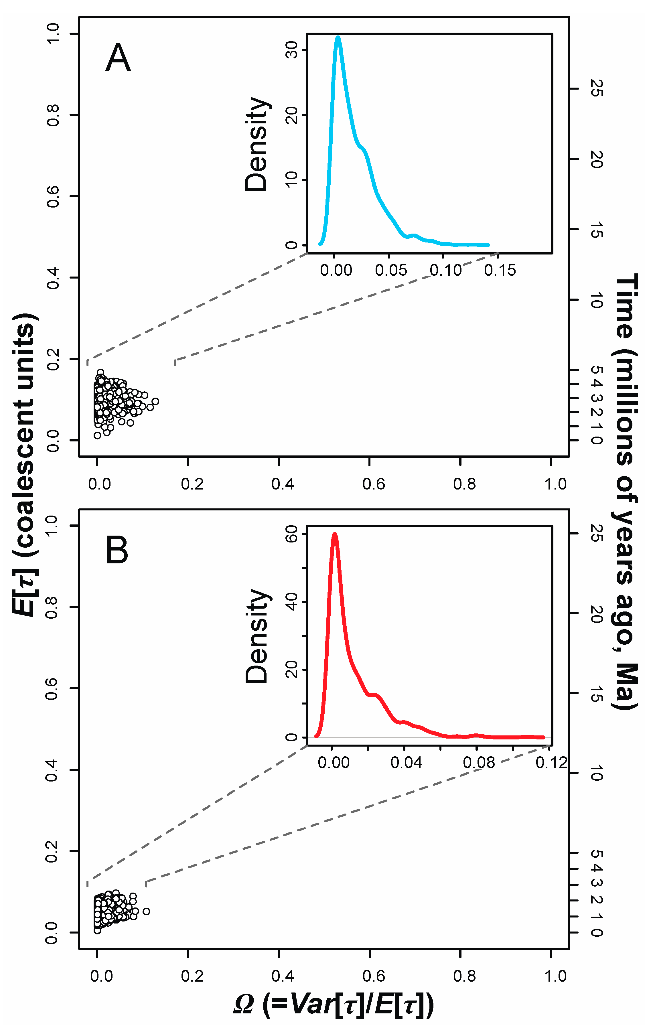
3.3. Tests for Synchronous Diversification

Projecting the observed data into principal components calculated from summary statistics randomly drawn from each model class showed that MTML-msBayes efficiently sampled our prior distributions (Figure S1). Observed data points also had similar positions across model classes, suggesting different priors were similarly good samplers for the data. Below we report results based on Ω posteriors derived from local linear regression [21].
We found that the modes of model-averaged posterior estimates of hyperparameter Ω were consistent with synchronous divergences within the frog and fish assemblages (frog Ω mode = 0.0036; fish Ω mode = 0.0017; Table 2; Figure 5). In agreement with this pattern, Ω = 0 fell within the credible intervals (95% HPD) of each of the model-averaged Ω distributions. The best-supported models also indicated synchronous divergence of the frog and the fish lineages based on posterior modal Ω values of 0.0013 and 0.0047, respectively. Despite this, model comparisons using Bayes factors for the ABC model-averaging results indicated that the data provided equivocal support for or against either model. Bayes factors were around a value of 1 for both the synchronous diversification model (frog B10 = 1.14 for Ω < 0.01 versus Ω > 0.01; fish B10 = 1.33 for Ω < 0.01 versus Ω > 0.01) as well as the asynchronous diversification model (frog B10 = 0.88 for Ω > 0.01 versus Ω < 0.01; fish B10 = 0.75 for Ω > 0.01 versus Ω < 0.01). Bayes factors were technically less than 1 for two or more divergences, but at best this provides very weak negative evidence for asynchronous divergence [72,73]. Likewise, posterior probabilities for the best-supported models were low (<0.5) and corresponding Bayes factors for synchronous diversification were weak, being approximately less than or equal to 1.
Based on model-averaging, the modes of assemblage E[τ] for the frog lineages and fish lineages were 0.106 (95% HPD = 0.056–0.139) and 0.054 (95% HPD = 0.022–0.079), respectively (Figure 5). When converted to absolute time using the median frog and fish mutation rates above, these peak-likelihood estimates correspond to modal dates of 3.09 Ma (95% HPD = 1.62–4.03 Ma) in the Pliocene to early Pleistocene for the frog divergences and 1.36 Ma (95% HPD = 0.56–2.021 Ma) in the early-mid Pleistocene for the fish divergences (Figure 5).

4. Discussion

4.1. Comparative Phylogeography of Panamanian Frog and Fish Assemblages

Determining whether species assemblages experienced shared evolutionary responses to historical geological and climate-change events is a central but challenging goal of comparative phylogeography [2,6,10]. Multi-taxon hABC methods for comparative phylogeography, for example, [22,23,24,25], permit testing explicit hypotheses about the timing of genetic divergences that have arisen during the assembly and diversification of regional species assemblages [26,27,28,29,30,31,33]. We used hABC coalescent models and full-Bayesian divergence dating to investigate temporal patterns of diversification of frogs and freshwater fishes across the WPI phylogeographic break (Figure 1 and Figure 2; [5]) to test two a priori hypotheses about the origin of species distributions and genetic structuring along the Pacific coast of Panama.
Several aspects of our results indicated that the frog and freshwater fish assemblages each experienced a synchronous pulse of diversification in this region during the late Neogene to Quaternary. This was supported by overlap in estimated tMRCAs for the taxon-pairs (Figure 4), strong peaks in the Ω posteriors near zero (Figure 5) and credible intervals including zero (Table 2), and peak-likelihoods and credible intervals of assemblage E[τ]. By contrast, Bayes factor model selection indicated that the data provide only a marginal accumulation of evidence in favor of synchronous diversification and against the null scenario of asynchronous diversification. The msBayes approach has been shown to correctly reject synchronous diversification using only mtDNA and summary statistics such as those used herein (e.g., [23,24,25]), and visual checks suggested that our priors were efficient samplers of the data (Figure S1). Moreover, we avoided the problem of overly broad or narrow τ priors (e.g., in [26,32]), which can cause ABC samplers to explore parameter space exceeding saturation effects on mitochondrial genes [24], by matching the upper bounds of these priors to empirical estimates from the data. As a result, we conclude that additional genetic data from unlinked loci or additional species, or improved methods for hABC or Bayes factor estimation, are needed to more confidently assess the timing and number of events at the WPI break in these taxa. Nevertheless, the much narrower credible intervals of our assemblage divergence times relative to the Bayesian gene-tree depths inferred in BEAST (Figure 3 and Figure 4) indicate that accounting for coalescent processes and changes in population sizes through time in our models yielded much more precise estimated divergence times across the WPI break than were previously available. Assuming that peaks in Ω and E[τ] contain one or multiple clusters of population divergence events, and acknowledging limitations and caveats of our mtDNA data (see Introduction and Section 4.2 below), we use our Bayesian assemblage E[τ] estimates to draw broad conclusions about the timing of diversification in these two assemblages and conduct hypotheses tests. We also discuss implications of our results for understanding the historical biogeography and diversification of Panamanian frog and freshwater fish species assemblages.
The dry forest hypothesis predicts that the timing of diversification of frogs across the WPI break was marked by the transition from wet tropical forest in the middle Cenozoic to drier forest habitats along the Pacific coast of Panama by >4 Ma according to paleobotanical data [44,45], and up to 12 Ma based on mtDNA phylogenetic dating analyses [42,43]. Against these predictions, we inferred that frog diversification across the WPI break occurred more recently, around 3.09 Ma (Figure 3 and Figure 4). Credible intervals for model-averaged assemblage E[τ] from MTML-msBayes slightly overlapped the predicted interval, by only ~31 thousand years (kyr); thus, we do not reject the dry forest hypothesis outright. However, modal Ω and assemblage E[τ] estimates favor the conclusion that the fracturing of western and eastern Pacific Panama frog assemblage coincided with one or multiple historical events occurring after 4 Ma, during the late Pliocene–early Pleistocene. Differences between frog divergence times inferred by earlier workers and this study likely owe in part to differences in sampling and methods used. Crawford et al. [42] dated the isolation of Golfo Dulce Craugastor populations using analyses that combined interspecific samples and employed strict molecular-clock and nonparametric rate smoothing methods. Thus, unlike population divergence times we estimated in MTML-msBayes, earlier estimates of Golfo Dulce frog divergence times were based on gene divergences, which are more apt to overestimate the timing of diversification, for example [12].
While we cannot reject the dry forest hypothesis outright, our results are more consistent with the interpretation that Plio–Pleistocene sea level highstands limited frog dispersion and gene flow across the region, as predicted by the Bermingham/Martin model [9]. The Pliocene warm period was a time of reduced global ice volume, stable and warmer temperatures, and widely fluctuating sea levels 3.5–2.5 Ma [47,75]. Geological evidence from deep-sea sediments and passive continental margins shows that a Pliocene sea-level highstand +35 ± 18 m above present sea levels (a.s.l.) occurred 3.5–3 Ma [47,76] and swept over the emerging central Panama isthmus just prior to its final formation around ~2.8 Ma ([46,47,77]; but see [78]). Our divergence time estimates from MTML-msBayes place diversification in the frog assemblage around the time of this eustatic highstand (it falls within the Bayesian credible intervals completely) and match closest to its lower boundary (Figure 4).
To provide a post-hoc test of whether a Pliocene eustatic highstand could have isolated frogs across the WPI break based on external geographical data, we developed a geographic information systems (GIS) model of sea-level rise over the NASA Shuttle Radar Topographic Mission 250 m resolution digital elevation model (CGIAR-CSI; available at: http://srtm.csi.cgiar.org) using ArcMap version 10 (ESRI, Redlands, CA, USA). The model was constructed by tracing the 50 m, 100 m, and 250 m elevation contours at high resolution, similar to [5,79]. Assuming the upper limit of Cronin and Dowsett [47], the GIS sea-level model suggests that a highstand ~+50 m a.s.l. could have inundated the coastal plain between Golfo Dulce and Soná peninsula, the valley between Soná and Azuero peninsulas, and much of the east coast of Azuero peninsula, isolating it from central Panama (Figure 6). This model is conservative, given that lower Central American lands approached their modern subaerial extent by at least mid-late Pliocene if not earlier (see [78]), and the Pliocene Panama landscape was likely lower and more topographically homogeneous than the present-day landscape (reviewed by [5,44,80]). We hypothesize that the WPI break was subsequently reinforced by the mid-Pleistocene eustatic highstand ~550–390 ka, when sea levels were +22 m a.s.l. [77,81]. Relative to the dry forest hypothesis, this ‘marine vicariance hypothesis’ presents a testable and non-mutually exclusive hypothesis that explains how a eustatic highstand might have sparked multiple responses to a single period of sea-level rise and maintained any previous genetic divergence at the WPI break originally created by expansion of dry forests.
Within the Panamanian frog assemblage, lineage dispersal and persistence appear to be at least partly controlled by ecological requirements and degree of specialization, as well as life-history mode. For example, E. pustulosus is a generalist occurring in savannahs and open environments as well as humid and dry forests [40]. In our results, this species exhibited the youngest divergence across the WPI (Figure 3 and Figure 4), possibly reflecting greater capacity to disperse and establish populations in different habitats, or exchange genes with other populations. That said, the degree of genetic admixture among Panamanian populations of E. pustulosus is poorly understood, and has only previously been documented by nuclear allozymes [51]. Dendropsophus ebraccatus and A. callidryas are ecologically similar species ([40,53], refs. therein) and display broadly overlapping tMRCAs slightly older than that of E. pustulosus but younger than that of C. crassidigitus (Figure 3). In turn, C. crassidigitus (like C. talamancae) is considered more ecologically specialized, preferring wet forest habitat more so than its dry-forest congeners (i.e., C. fitzingeri; [42]). That the C. crassidigitus gene tree extends farthest backward in time thus seems to suggest this species experienced long-term isolation and persistence in preferred habitats, rather than an ability to tolerate climatic or vegetational shifts. However, whereas all the other frog species are egg-layers, Craugastor dirt frogs are direct-developing species that readily reproduce, and their local population sizes can therefore be notoriously large [82]. Given the direct relationship between Ne and time to coalescence from coalescent theory, this contrast in life-history strategies would suggest that on one hand C. crassidigitus may have been superior at colonizing open niches or patches and spread throughout isthmian wet forest habitats more easily than the other taxa, while on the other hand its tMRCA estimate may also be inflated due to large ancestral Ne [19].
Freshwater fishes typically exhibit higher levels of mtDNA sequence divergence and endemism in Atlantic relative to Pacific drainages of the Isthmus of Panama [9]. On the Pacific versant, the ~124 km-wide Gulf of Panama continental shelf (Figure 1) would have been broadly exposed as eustatic sea levels lowered 110–135 m during the Last Glacial Maximum (LGM, ~21 ka) and other glaciations, for example [75]. The above pattern likely owes to greater opportunities for dispersion and gene flow between drainages that coalesced over Pacific shelf areas during Pleistocene glacial periods [9,80]. Yet, this trend breaks down slightly in western Panama, where freshwater fishes show distinct associations between biogeography and phylogeography. Despite low endemism within fish provinces, geographical ranges of 14 fish species terminating at Soná and Azuero peninsulas (Figure 1) support a boundary between the Chiriquí and Santa Maria fish biogeographical provinces at the Río Santa Maria, Soná peninsula [80]. The WPI genetic break occurs in the same area in freshwater fishes (Figure 2C,D). Thus, historical processes importantly shaped Panamanian fish species turnover and diversification at the WPI break zone. Yet what mechanism best explains the isolation of fishes across the WPI break?
The Bermingham/Martin model predicts that WPI breaks in fishes have resulted from the isolation of fish populations west of Soná peninsula from those between Soná peninsula and El Valle volcano during glacial periods with sea-level lowstands since 2 Ma in the Pleistocene [9]. Consistent with this model, we found that the lower 95% HPDs for tMRCA estimates for all three fish species/lineages fell within the predicted interval of diversification (Figure 3 and Figure 4). Peak posterior distributions from hABC model-averaging (e.g., Figure 5) also suggested that the focal fish species/lineages most likely diversified across the WPI break 1.36 Ma in the early Pleistocene, with Bayesian credible intervals ranging from early–late Pleistocene. This time period correlates best to the ‘Calabrian’ age (1.806–0.781 Ma; [83]), a time of 41-kyr periodicity of Pleistocene glaciations with drier and cooler-than-present conditions but less-extreme climatic oscillations than those following 800 ka [75,84]. Nevertheless, glacial periods vastly dominated the Calabrian to present, such that the Panama isthmus would have experienced many glacio-eustatic cycles but spent the majority of time since 1.8 Ma under glacial conditions with lowered sea levels and exposed continental shelf habitats. Eustatic sea-level curves give no convincing evidence that the oceans reached modern sea levels for any substantial period of time (e.g., >10–20 kyr) since the Calabrian, and the next eustatic sea-level highstand is not registered in the geological record until ~550–390 ka [76,81]. Geological patterns and processes are also consistent with decreased likelihood of fish dispersal across the WPI break zone since the Calabrian. In the break zone, the Pacific continental shelf becomes narrower (~0–40 km), tapering to the western Azuero peninsula coastline before being bisected by Cébaco and Coiba islands at the nearby Gulf of Montijo draining Soná peninsula (Figure 1). To evaluate the impact of lowered sea levels during Pleistocene glaciations on drainage connectivity in this area, we obtained a GIS model predicting paths of LGM paleo-drainages over modern bathymetry using ArcMap (courtesy of Peter J. Unmack, University of Canberra). The GIS model suggests that rivers draining to the west versus east of Soná peninsula did not anastomose over the continental shelf during the LGM (Figure 1), and possibly also preceding glaciations. Overall, our results combined with external environmental data suggest that a relatively stable geological setting at the Soná peninsula barrier has aided the historical isolation of drainage basins, maintaining fish lineage divergences at the WPI break during lower seas of the Calabrian to present.
While this study chiefly focuses on comparative phylogeographic modeling of codistributed Panamanian frogs and freshwater fishes, these assemblages also provide a system with ecological affinities (e.g., associations with freshwater pools and streams) and contrasts (terrestrial versus freshwater habits) making them suitable for assessing possible influences of the degree of ecological differentiation on phylogeographic structuring. One obvious ecological pattern among our results is that, at the deepest phylogenetic and ecological division among taxa in our study, frogs and fishes may have experienced largely independent pulses of diversification in the WPI break zone. Divergence events in these assemblages are not entirely statistically independent, given the overlapping credible intervals of their divergence times (Figure 3 and Figure 4), and our analyses treated these assemblages separately. However, the two-fold difference in the peak-likelihood E[τ] estimates suggest that frogs and freshwater fishes may have responded differently to the fluctuating paleogeographic, geologic, and climatic context of western Pacific Panama, for example [10]. We recommend that this hypothesis be tested using hABC models for comparative phylogeography improved by additional sampling (taxa and loci) and methodological improvements increasing the resolution of the models. However, under this scenario, dispersal of different lineages would be more strongly controlled by differences in ecological requirements among, rather than within, the two species assemblages. Thus, a potential biogeographical explanation for why these assemblages might have failed to register the impact of the same historical events is that the focal frog species/lineages, but not the fish lineages, colonized the Pacific coast of Costa Rica and Panama prior to the Pliocene eustatic highstand event, which left a greater signature on their genotypes than subsequent historical processes. This is supported by phylogenetic dating analyses of one frog lineage that we evaluated, the Craugastor fitzingeri group containing C. crassidigitus, which likely colonized the Central American Isthmus in the Eocene–early Miocene from a South American source population [58].

4.2. Caveats and Potential Limitations

4.2.1. Mitochondrial DNA

Our study makes several novel contributions, for example by providing the first hABC modeling study illuminating comparative phylogeography of both terrestrial and freshwater species assemblages from the Isthmus of Panama. There are limitations to an approach based solely on mtDNA, as also discussed in the Introduction. Therefore, we have provided a cautious interpretation of our results with the following limitations and caveats in mind.First, our hABC modeling analyses in MTML-msBayes accounted for coalescent stochasticity of the genetic data by allowing rates of lineage sorting to vary among population-pairs, but if multiple unlinked nuclear loci had been available to us, these may have allowed us to improve our accounting for the stochastic variance of coalescent processes and arrive at more accurate estimates of divergence times or other parameters, for example [12,85,86]. Even so, previous simulation tests of MTML-msBayes using pseudo-observed datasets from five taxon-pairs show that a single locus outperforms smaller multilocus datasets [25]. Significant improvements (i.e., lower root mean square error, RMSE) in estimating hyperparameters Ω and E[τ] only come when the total number of unlinked loci reaches ≥16, and additional increases in estimator accuracy require greater than 32 loci [25]. As a result, given that we analyzed mtDNA collected in studies conducted over a 14-year period (Table 1), it will likely take several more years before phylogeographic datasets from multiple Panamanian frog and freshwater fish taxa are sufficiently large to improve upon our results by scaling available datasets up to ≥16–32 loci. Moreover, if nuclear loci indicate substantial recombination, incomplete lineage sorting, or admixture across the WPI break, then these will pose additional analytical challenges and, particularly in the case of including migration parameters [22,25], are likely to require many more unlinked nuclear loci to develop models that perform well. One reason for this is that substantial migration can hinder the msBayes model from accurately inferring or rejecting simultaneous diversification, for example [22].
A second caveat to our results is that they may have been influenced by errors in the mutation rates supplied to the software programs. We conservatively identified ranges of plausible mutation rates for protein-coding mtDNA genes in frogs and fishes, and used these to set uniform priors on μ parameters in BEAST and MTML-msBayes. In each case, we allowed the software to estimate μ, through ABC or MCMC inference, and we allowed μ values to vary among population-pairs. Thus, our analyses accounted for potential differences in μ among species/lineages, especially when estimating gene-tree depths in BEAST. However, had more accurate estimates of mtDNA divergence rates been available, our estimates of species/lineage and assemblage divergence times could have been more accurate, and we could have been able to reduce the number of parameters in our models by fixing the mutation rates to accurate estimates for each species/lineage, mainly in the case of BEAST. If, however, mutation rates are broadly similar among taxa as our μ priors assume but the prior ranges were off by some particular factor (e.g., by half, or two-fold), then we would expect to have obtained similar results during our tests for simultaneous diversification under different μ priors, correcting by that factor. We also note that the original studies that produced the datasets we analyzed (see Table 1) estimated lineage divergence times using methods that infer gene divergence times from single loci. Their results are thus more likely to have overestimated the timing of lineage divergences across the WPI break than our methods, which only estimated population divergence times, for example [12].
A third caveat is that, while our datasets met the assumption of mtDNA neutrality (see Results and Appendix A.2.1 of Appendix A), we have made assumptions about species demographic histories in each of our analyses that are common to many studies, but that may have introduced error into the results. For example, in BEAST we set constant population size tree priors assuming the entire sample including both daughter populations for each population-pair evolved under the neutral coalescent with constant population size through time [19]. However, in MTML-msBayes, ancestral population size segments that evolved within each daughter population were assumed to experience exponential population growth to present. Additional demographic information and more flexible modeling approaches allowing different population-size transitions in different parts of the population trees for each population-pair, had they been available, may have permitted more accurate demographic models yielding more accurate parameter estimates. Nevertheless, although we allowed population size changes in our models, our main goal was not to infer historical demography of each species, at large.

4.2.2. Migration and “Secondary Contact”

A demographic model of “secondary contact” would include a period of pure genetic divergence, with two lineages initially diverging in the absence of gene flow and then experiencing relatively recent secondary contact. We did not include this kind of model because it is not available in the state-of-the-art comparative phylogeography software pipeline that we used. The MTML-msBayes implementation of the msBayes hABC pipeline that we used incorporates two models: a pure divergence model, or “isolation model”, and a migration model [25]. The latter model is an isolation-with-migration type model, in which migration parameters (Nm) are included for each of the Y taxon/species pairs in the analysis (Table A1; Figure S2), and migration is allowed to vary among each of these pairs from the time of initial divergence to the present (except this occurs backwards in time, since the software uses a coalescent model); thus, this model is similar but not equivalent to a scenario of secondary contact.
We also did not include migration parameters in our MTML-msBayes analyses. The reason for this is that there is essentially zero evidence supporting genetic patterns reflecting incomplete lineage sorting or migration across the western Panama Isthmus (WPI) break among datasets analyzed in our paper. In fact, only one study focusing on just one of the seven species/lineages that we evaluated previously inferred any admixture or migration between WPI lineages—in the case of the frog, Engystomops pustulosus, based on admixture signals in nuclear allozyme data [51]. In total, ~86% of the lineages that we evaluated in the present paper are completely sorted across the WPI break, with no mtDNA evidence for interpopulation gene flow across the break zone (Figure 2 and Figure 3). Under the MTML-msBayes migration model, all lineages diverge in the presence of gene flow, and their migration rates are drawn from the same uniform prior, for example parameterized with Nm ~U(0, 1.0) meaning that migration is allowed to vary up to one individual per generation [28]. Incorporating migration rates into multi-species analyses of co-diversification in the MTML-msBayes pipeline is thus inappropriate for our data, and would likely have had adverse effects on model performance. This is because using migration models would force the software to estimate additional migration parameters for species pairs for which there is no data signal that is informative for migration (e.g., alleles shared between diverging species/lineages), and this could theoretically result in incorrect estimation of population size (θ) and divergence time (τ) parameters.
The effects of migration on MTML-msBayes analyses are fairly well known, and our decision not to include migration in our models is supported by several previously published studies. In particular, in a paper presenting the updated MTML-msBayes version of the msBayes pipeline, Huang et al. [25] showed through simulation that hyperposterior results were less accurate when migration was included in the model (isolation with migration, not secondary contact), but the hyperposteriors, hence inferences, were improved when the correct migration model was specified. For example, simulating with migration when the data were known to be from a model with no migration (Nm = 0) yielded hyperposterior Ω (divergence time variance) and E[τ] (divergence time) estimates with much wider variance (RMSE), obscuring interpretation (see Figures 6 and 7 in [25]). Additionally, Bell et al.’s [28] recent comparative phylogeography study of codistributed frog species from the Australian Wet Tropics inferred patterns of population structure similar to those we see in frogs and fishes across the WPI break in Panama, with their Figure 1 showing genetic evidence for allele sharing or potential migration/admixture in only one (20%) of five frog species surveyed. They used Bayes factors [73] to compare MTML-msBayes models with and without migration, and their mtDNA-only results from analyzing data very similar to ours overwhelmingly supported isolation models [28]. Adding a small number of nuclear markers also did not cause migration models to fit better than isolation models for the majority of species in their dataset [28]. Given similarities between data and phylogeographical patterns in our study and Bell et al.’s [28], it seems reasonable to expect that comparing isolation and migration models using our data would yield similar results.
There are two additional points about migration of relevance to our MTML-msBayes analyses. First, the MTML-msBayes framework is not highly robust to migration, as migration can increase gene tree variance, such as variation in tree shape or depth [87], and in theory should reduce resolution of hABC inference. However, there is some evidence that MTML-msBayes is increasingly robust to errors in estimating the main hyperparameters of the model, Ω and E[t], with increasing amounts of data (numbers of loci), with or without migration. Still, simulations show that increases in estimator accuracy mainly occur when the number of independent, unlinked markers rises above 16 loci (see Figures 3A and 4A in [25]). There are no additional nuclear markers available for the codistributed taxa that we have studied in the present paper, and we are unaware as to whether any additional data will become available for these species in the foreseeable future. Thus, our paper is not only the first to provide a synthesis of the available data, but the data analyzed are also the best data available to address the questions and hypotheses that we focus on in our manuscript, using an appropriate framework for comparative phylogeography.

5. Conclusions

We conducted the first tests for simultaneous diversification of frogs and fishes at the WPI break in western Panama (reviewed by [5]) by analyzing mtDNA sequences using ABC methods accounting for uncertainty in model selection using modeling averaging [24,25]. Current findings show that, despite good prior selection and sampling properties (also supported for our datasets by simulations in [37]), hABC tests for synchronous diversification using mtDNA datasets remain challenging and difficulties can arise in conducting hypotheses tests based on Bayes factors when analyzing small numbers of taxon/population-pairs. However, our study also demonstrates that, in such cases, integrating assembly-wide divergence time estimates, E[τ], from hABC with external information from geology and elevation data can still generate novel biogeographical insights and hypotheses towards refining the existing biogeographical context for a region, even despite the limitations of mtDNA (see Introduction and Discussion Section 4.2.1). Recent advances in hABC analysis, including extensions to genome-wide single nucleotide polymorphism (SNP) data [88,89] and better inference through buffering multi-taxon divergence times [37], suggest an exciting period ahead for comparative studies of the diversification of vertebrate species assemblages in Panama and other Neotropical ‘hotspots’. We encourage future phylogeographic studies of the frog and fish taxa analyzed herein, and other Panamanian taxa, to build upon the present foundation by developing and analyzing datasets with increased taxon and character sampling, while capitalizing on these computational advances. A particularly fruitful way forward in future examinations of the WPI break would be to develop SNP datasets, for example using ddRAD-seq [90], and then test for co-demographic expansion and co-diversification using aggregate site frequency spectrum methods [89]. Such approaches should provide the increased power and resolution needed to more confidently identify the number and timing of divergence events that have shaped vertebrate diversification across the WPI break, and other multi-taxon genetic breaks along the Isthmus of Panama.

Supplementary Materials

The following are available online at https://www.mdpi.com/1424-2818/10/4/120/s1, Table S1: GenBank numbers and locality data for samples used in this study, Figure S1: Graphical checks on prior distributions listed in Table 1 based on principal components analysis. Red dots show the observed data for (A) frogs and (B) freshwater fishes projected into the principal components space, Figure S2: Summary of the general coalescent model implemented in MTML-msBayes, including model parameters. This model is replicated and parameters are allowed to vary across Y taxon/population-pairs, which experience from 1 to Ψ independent divergence events (see additional parameter details in Table A1 of Appendix A).

Author Contributions

Conceptualization, J.C.B. and J.B.J.; Data curation, J.C.B.; Formal analysis, J.C.B. and M.J.H.; Investigation, J.C.B.; Methodology, M.J.H.; Project administration, J.B.J.; Resources, J.B.J.; Software, J.C.B. and M.J.H.; Supervision, J.B.J. and M.J.H.; Validation, M.J.H.; Visualization, J.C.B. and M.J.H.; Writing—original draft, J.C.B.; Writing—review & editing, J.B.J. and M.J.H.

Funding

Justin C. Bagley was funded in part by a Graduate Research Fellowship from Brigham Young University (BYU) Graduate Studies, and by a National Science Foundation (NSF) Doctoral Dissertation Improvement Grant (DEB-1210883; to Jerald B. Johnson and Justin C. Bagley). There was no additional external funding received for this study.

Acknowledgments

We thank María Florencia Breitman, Andrew J. Eckert, Michael J. Ryan, Graham Wallis, Michael Wink, and two anonymous reviewers for helpful discussion and comments on earlier drafts of this manuscript. We thank Peter J. Unmack for providing paleo-bathymetric river data aiding interpretation. We also thank the Brigham Young University Fulton Supercomputing Lab for providing generous computational resources.

Conflicts of Interest

The authors declare no conflict of interest. The funders had no role in the design of the study; in the collection, analyses, or interpretation of data; in the writing of the manuscript; or in the decision to publish the results.

Appendix A

Appendix A.1. Supplementary Methods

Appendix A.1.1. Taxon Sampling, Molecular Data, and Outgroup Details

Here, we provide additional information on sampling, DNA sequence data, and outgroup taxa used in our analyses that we were unable to give in the main text due to space limitations. First, the majority of our analyses did not include outgroup taxa; this majority includes the nucleotide diversity and % divergence calculations, estimating tMRCAs in BEAST, tests for simultaneous diversification in MTML-msBayes, and our IMa2 analyses of community divergence. However, it was necessary to specify outgroup taxa in our analyses evaluating whether the data were consistent with predictions of the neutral model of molecular evolution [91]. To this end, we conducted MK tests, which test for deviations of the ratio of replacement (nonsynonymous fixed; RI) to synonymous fixed (SI) substitutions within species from that between species. Specifically, the SI:RI ratio from patterns of substitutions within one species (e.g., one of our focal population-pair datasets) is compared with that of the between-species patterns yielded from comparison to a close relative (e.g., a congeneric outgroup or sister species of one of our focal taxa). In the implementation of the MK test in DnaSP, substitution patterns in an intraspecific dataset are compared against the one or multiple sequences in an outgroup species dataset, and a non-significant difference between the two rations based on two-tailed Fisher’s exact tests is taken as evidence of neutrality. Next, we list outgroups used in MK tests for each population-pair dataset as well as references to studies used to determine the appropriate outgroups. We also provide GenBank accession numbers for outgroup sequences in parentheses, and all outgroup sequences were homologous to those of the focal taxon dataset. Based on phylogenetic analyses in Robertson et al. [54] and Robertson & Zamudio [53], we used one 16S-ND1 sequence of the congener Agalychnis saltator (GenBank GQ366296, [92]) in our MK test of the A. callidryas dataset. Based on phylogenetic analyses in Crawford et al. [42], we used 12 composite cytb-cox1 sequences of the congener Craugastor fitzingeri (GenBank DQ350193–198, DQ350236–241, [42]; EF635371, EF629419–423, EF629462, EF629458, EF629459, EF629455, EF629453, other studies cited in [42]) in our MK test of the C. crassidigitus dataset. Based on Robertson et al. [54], we used one composite sequence of 16S, tRNA-Leu, and ND1 genes from the congener Dendropsophus microcephalus (GenBank AY819503, [93]) as the outgroup in our MK test of the D. ebraccatus dataset. Based on Weigt et al. [51], we used one congeneric Engystomops petersi cox1 sequence from that same study (GenBank DQ120042) as the outgroup in our MK test of the E. pustulosus dataset. Based on McCafferty et al. [54], we used eight ATPase6/8 sequences from congener Andinoacara rivulatus (GenBank JX677777–784, [94,95]) as the outgroup sequences in our MK tests of the A. coeruleopunctatus dataset. Based on results in Bermingham and Martin [9] and Martin and Bermingham [55], we used composite ATP6/8, cox1 sequences from six individuals of the “type B” Pimelodella chagresi lineage (a cryptic species lineage discovered in that study; GenBank AF040388, AF040407–409, AF040412, AF040415, AF040484–489) as the outgroup sample in our MK test of the P. chagresi population-pair dataset. Last, based on Bermingham and Martin [9], we used composite ATP6/8, cox1 sequences from three individuals of the congener Roeboides meeki (GenBank AF040522–524 and AF040559–561 [9]) as the outgroup sample in our MK test of the R. occidentalisR. guatemalensis population-pair dataset.

Appendix A.1.2. Supplementary MTML-msBayes Methods

Below, we supplement our presentation of MTML-msBayes methods above by providing a summary of the parameters and prior distributions of the model [22,25], including the default prior distributions of each parameter (Table A1). To further aid understanding of the model, we also provide a matching graphical summary of the basic demographic model in Figure S2 of the Supplementary Materials. However, as noted in the main text (see Discussion Section 4.2.2), we did not include the migration parameters in our analysis.

Appendix A.2. Supplementary Results

Appendix A.2.1. Additional Genetic Diversity and Neutrality Results and Discussion

Based on p-values from Fisher’s exact tests, our MK tests did not detect significant (p < 0.05) departures from mtDNA neutrality in any of the WPI break population-pair-to-outgroup comparisons: A. callidryas p = 0.271; C. crassidigitus p = 0.620; D. ebraccatus p = 0.449; E. pustulosus p = 0.116; A. coeruleopunctatus p = 1.000; p. chagresi p = 1.000; R. occidentalisR. guatemalensis p = 0.104.

Appendix A.2.2. Additional MTML-msBayes Results and Discussion

The posterior distribution of the divergence time parameter showed relatively small amounts of variance, or Var[τ], in both analyses of the frogs (M2 mode Var[τ] = 3.89 × 10⁻⁴; model-averaging Var[τ] = 3.85 × 10⁻⁴, estimated from hyperparameter modes) and freshwater fishes (M2 mode Var[τ] = 0.0015; model-averaging Var[τ] = 9.63 × 10⁻⁵, estimated from hyperparameter modes). However, variance of the modal τ values from model averaging was greater than that from the best-supported models.
Table A1. Summary of generic MTML-msBayes model parameters for Y taxon/population pairs and their prior distributions (modified from [23,25]).
ParameterDescriptionPrior Distribution
A. Hyperparameters
ΩDispersion index of divergence times, Var[τ]/E[τ] (ratio of variance to mean), across Y taxon/population-pairsSet by Y, τmax, and Ψ
E[τ]Mean multi-species (i.e., assembly-wide) divergence time across YSet by Y, τmax, and Ψ
ΨNumber of distinct divergence times across YDiscrete uniform [1, Y]
SVector of mutation rate scalars to accommodate among-locus mutation rate heterogeneityGamma (with shape and scale parameters α and 1/α, respectively)
αShape parameter of the gamma distributionUniform (1, 20)
B. Parameters
τDivergence time in units of 4N generationsUniform (0.0, τmax)
θ = 4Population size (mutation) parameter where N is average population size of two daughter populations, µ is the per-site mutation rateUniform (θmin, θmax)
θAAncestral effective population size (mutation) parameterUniform (0.01, θmax Nanc-max)
θA1, θA2Ancestral effective population size (mutation) parameters for daughter populations 1 and 2 over ancestral period (from time τ to τB)Uniform (0.01, θB1), (0.01, θB2)
θB1, θB2Effective population size (mutation) parameters for daughter populations 1 and 2 over recent period (from time τB to 0.0, the present time)Uniform (0.01 θ, 1.99θ), and where θB2 = 2θθB1
τB1, τB2Times at which θA1 and θA2 experience exponential growth into populations with sizes of θB1 and θB2Uniform (0.0, τ), with τB1 = τB2
M = NmEffective migration rate, where m is the probability of symmetric migration between pairs of daughter populationsUniform (0.0, Mmax)
rPer-locus mutation rate scalarfixed
pPer-locus ploidy and/or generation time scalarp

References

  1. Avise, J.C.; Arnold, J.; Ball, R.M.; Bermingham, E.; Lamb, T.; Neigel, J.E.; Reeb, C.A.; Saunders, N.C. Intraspecific phylogeography: The mitochondrial DNA bridge between population genetics and systematics. Annu. Rev. Ecol. Syst. 1987, 18, 489–522. [Google Scholar] [CrossRef]
  2. Avise, J.C. Phylogeography: The History and Formation of Species; Harvard University Press: Cambridge, MA, USA, 2000. [Google Scholar]
  3. Kidd, D.M.; Ritchie, M.G. Phylogeographic information systems: Putting the geography into phylogeography. J. Biogeogr. 2006, 33, 1851–1865. [Google Scholar] [CrossRef]
  4. Soltis, D.E.; Morris, A.B.; Jason, M.; McLachlan, S.; Manos, P.S.; Soltis, P.S. Comparative phylogeography of unglaciated eastern North America. Mol. Ecol. 2006, 15, 4261–4293. [Google Scholar] [CrossRef] [PubMed] [Green Version]
  5. Bagley, J.C.; Johnson, J.B. Phylogeography and biogeography of the lower Central American Neotropics: Diversification between two continents and between two seas. Boil. Rev. 2014, 89, 767–790. [Google Scholar] [CrossRef] [PubMed]
  6. Arbogast, B.S.; Kenagy, G.J. Comparative phylogeography as an integrative approach to historical biogeography. J. Biogeogr. 2001, 28, 819–825. [Google Scholar] [CrossRef]
  7. Hickerson, M.J.; Carstens, B.C.; Cavender-Bares, J.; Crandall, K.A.; Graham, C.H.; Johnson, J.B.; Rissler, L.; Victoriano, P.F.; Yoder, A.D. Phylogeography’s past; present; and future: 10 years after Avise. 2000. Mol. Phylogenet. Evol. 2010, 54, 291–301. [Google Scholar] [CrossRef] [PubMed]
  8. Bermingham, E.; Avise, J.C. Molecular zoogeography of freshwater fishes in the south-eastern United States. Genetics 1986, 113, 939–965. [Google Scholar] [PubMed]
  9. Bermingham, E.; Martin, A.P. Comparative mtDNA phylogeography of Neotropical freshwater fishes: Testing shared history to infer the evolutionary landscape of lower Central America. Mol. Ecol. 1998, 7, 499–517. [Google Scholar] [CrossRef] [PubMed]
  10. Sullivan, J.; Arellano, E.; Rogers, D. Comparative phylogeography of Mesoamerican highland rodents: Concerted versus independent response to past climatic fluctuations. Am. Nat. 2000, 155, 755–768. [Google Scholar] [CrossRef] [PubMed]
  11. Avise, J.C. Gene trees and organismal histories: A phylogenetic approach to population biology. Evolution 1989, 43, 1192–1208. [Google Scholar] [CrossRef] [PubMed]
  12. Edwards, S.V.; Beerli, P. Perspective: Gene divergence; population divergence; and the variance in coalescence time in phylogeographic studies. Evolution 2000, 54, 1839–1854. [Google Scholar] [CrossRef] [PubMed]
  13. Hey, J.; Machado, C.A. The study of structured populations—New hope for a difficult and divided science. Nat. Rev. Genet. 2003, 4, 535–543. [Google Scholar] [CrossRef] [PubMed]
  14. Kuo, C.H.; Avise, J.C. Phylogeographic breaks in low-dispersal species: The emergence of concordance across gene trees. Genetica 2005, 124, 179–186. [Google Scholar] [CrossRef] [PubMed]
  15. Irwin, D.E. Local adaptation along smooth ecological gradients causes phylogeographic breaks and phenotypic clustering. Am. Nat. 2012, 180, 35–49. [Google Scholar] [CrossRef] [PubMed]
  16. Zink, R.M.; Barrowclough, G.F. Mitochondrial DNA under siege in avian phylogeography. Mol. Ecol. 2008, 17, 2107–2121. [Google Scholar] [CrossRef] [PubMed] [Green Version]
  17. Kubatko, L.S.; Carstens, B.C.; Knowles, L.L. STEM: Species tree estimation using maximum likelihood for gene trees under coalescence. Bioinformatics 2009, 25, 971–973. [Google Scholar] [CrossRef] [PubMed]
  18. Heled, J.; Drummond, A.J. Bayesian inference of species trees from multilocus data. Mol. Boil. Evol. 2010, 27, 570–580. [Google Scholar] [CrossRef] [PubMed]
  19. Hudson, R.R. Gene genealogies and the coalescent process. Oxf. Surv. Evol. Boil. 1990, 7, 1–44. [Google Scholar]
  20. Riddle, B.R.; Hafner, D.J. A step-wise approach to integrating phylogeographic and phylogenetic biogeographic perspectives on the history of a core North American warm desert biota. J. Arid. Environ. 2006, 66, 435–461. [Google Scholar] [CrossRef]
  21. Beaumont, M.A.; Zhang, W.; Balding, D.J. Approximate Bayesian computation in population genetics. Genetics 2002, 162, 2025–2035. [Google Scholar] [PubMed]
  22. Hickerson, M.J.; Stahl, E.; Takebayashi, N. msBayes: A pipeline for testing comparative phylogeographic histories using hierarchical approximate Bayesian computation. BMC Bioinform. 2007, 8, 268. [Google Scholar] [CrossRef] [PubMed]
  23. Hickerson, M.J.; Stahl, E.; Lessios, H.A. Test for simultaneous divergence using Approximate Bayesian Computation. Evolution 2006, 60, 2435–2453. [Google Scholar] [CrossRef] [PubMed]
  24. Hickerson, M.J.; Stone, G.N.; Lohse, K.; Demos, T.C.; Xie, X.; Landerer, C.; Takebayashi, N. Recommendations for using msBayes to incorporate uncertainty in selecting an ABC model prior: A response to Oaks et Al. Evolution 2014, 68, 284–294. [Google Scholar] [CrossRef] [PubMed]
  25. Huang, W.; Takebayashi, N.; Qi, Y.; Hickerson, M.J. MTML-msBayes: Approximate Bayesian comparative phylogeographic inference from multiple taxa and multiple loci with rate heterogeneity. BMC Bioinform. 2011, 12, 1. [Google Scholar] [CrossRef] [PubMed]
  26. Leaché, A.D.; Crews, S.C.; Hickerson, M.J. Two waves of diversification in mammals and reptiles of Baja California revealed by hierarchical Bayesian analysis. Boil. Lett. 2007, 3, 646–650. [Google Scholar] [CrossRef] [PubMed] [Green Version]
  27. Barber, B.R.; Klicka, J. Two pulses of diversification across the Isthmus of Tehuantepec in a montane Mexican bird fauna. Proc. R. Soc. Lond. B Boil. Sci. 2010, 277, 2675–2681. [Google Scholar] [CrossRef] [PubMed] [Green Version]
  28. Bell, R.C.; MacKenzie, J.B.; Hickerson, M.J.; Chavarría, K.L.; Cunningham, M.; Williams, S.; Moritz, C. Comparative multi-locus phylogeography confirms multiple vicariance events in co-distributed rainforest frogs. Proc. R. Soc. Lond. B Boil. Sci. 2011, 279, 991–999. [Google Scholar] [CrossRef] [PubMed] [Green Version]
  29. Dolman, G.; Joseph, L. A species assemblage approach to comparative phylogeography of birds in southern Australia. Ecol. Evol. 2012, 2, 354–369. [Google Scholar] [CrossRef] [PubMed] [Green Version]
  30. Bagley, J.C.; Johnson, J.B. Testing for shared biogeographic history in the lower Central American freshwater fish assemblage using comparative phylogeography: Concerted, independent, or multiple evolutionary responses? Ecol. Evol. 2014, 4, 1686–1705. [Google Scholar] [CrossRef] [PubMed]
  31. Smith, B.T.; Harvey, M.G.; Faircloth, B.C.; Glenn, T.C.; Brumfield, R.T. Target capture and massively parallel sequencing of ultraconserved elements for comparative studies at shallow evolutionary time scales. Syst. Boil. 2013, 63, 83–95. [Google Scholar] [CrossRef] [PubMed]
  32. Oaks, J.R.; Sukumaran, J.; Esselstyn, J.A.; Linkem, C.W.; Siler, C.D.; Holder, M.T.; Brown, R.M. Evidence for climate-driven diversification? A caution for interpreting ABC inferences of simultaneous historical events. Evolution 2013, 67, 991–1010. [Google Scholar] [CrossRef] [PubMed]
  33. Bagley, J.C. Understanding the Diversification of Central American Freshwater Fishes Using Comparative Phylogeography and Species Delimitation; Brigham Young University: Provo, UT, USA, 2014. [Google Scholar]
  34. Oaks, J.R. An improved approximate-Bayesian model-choice method for estimating shared evolutionary history. BMC Evol. Boil. 2014, 14, 150. [Google Scholar] [CrossRef] [PubMed]
  35. Oaks, J.R.; Linkem, C.W.; Sukumaran, J. Implications of uniformly distributed; empirically informed priors for phylogeographical model selection: A reply to Hickerson et al. Evolution 2014, 68, 3607–3617. [Google Scholar] [CrossRef] [PubMed]
  36. Papadopoulou, A.; Knowles, L.L. Species-specific responses to island connectivity cycles: Refined models for testing phylogeographic concordance across a Mediterranean Pleistocene Aggregate Island Complex. Mol. Ecol. 2015, 24, 4252–4268. [Google Scholar] [CrossRef] [PubMed]
  37. Overcast, I.; Bagley, J.C.; Hickerson, M.J. Improving approximate Bayesian computation tests for synchronous diversification by buffering divergence time classes. BMC Evol. Boil. 2017, 17, 203. [Google Scholar]
  38. Savage, J.M. The origins and history of the Central American herpetofauna. Copeia 1966, 1966, 719–766. [Google Scholar] [CrossRef]
  39. Savage, J.M. The enigma of the Central American herpetofauna: Dispersals or vicariance? Ann. Mol. Bot. Gard. 1982, 69, 464–547. [Google Scholar] [CrossRef]
  40. Savage, J.M. The Amphibians and Reptiles of Costa Rica: A Herpetofauna between Two Continents, Between Two Seas; University of Chicago Press: Chicago, IL, USA, 2002. [Google Scholar]
  41. Vanzolini, P.E.; Heyer, W.R. The American herpetofauna and the interchange. In The Great American Biotic Interchange; Stehli, F.G., Webb, S.D., Eds.; Plenum Press: New York, NY, USA, 1985; pp. 475–487. [Google Scholar]
  42. Crawford, A.J.; Bermingham, E.; Polania, C. The role of tropical dry forest as a long-term barrier to dispersal: A comparative phylogeographical analysis of dry forest tolerant and intolerant frogs. Mol. Ecol. 2007, 16, 4789–4807. [Google Scholar] [CrossRef] [PubMed]
  43. Wang, I.J.; Crawford, A.J.; Bermingham, E. Phylogeography of the pygmy rain frog (Pristimantis ridens) across the lowland wet forests of isthmian Central America. Mol. Phylogenet. Evol. 2008, 47, 992–1004. [Google Scholar] [CrossRef] [PubMed]
  44. Graham, A.; Dilcher, D. The Cenozoic record of tropical dry forest in northern Latin America and the southern United States. In Seasonally Dry Tropical Forests; Bullock, S.H., Mooney, H.A., Medina, E., Eds.; Cambridge University Press: Cambridge, UK, 1995; pp. 124–145. [Google Scholar]
  45. Piperno, D.R.; Pearsall, D.M. The Origins of Agriculture in the Lowland Neotropics; Academic Press: San Diego, CA, USA, 1998. [Google Scholar]
  46. Coates, A.G.; Obando, J.A. The geologic evolution of the Central American isthmus. In Evolution and Environment in Tropical America; Jackson, J.B.C., Budd, A.F., Coates, A.G., Eds.; University of Chicago Press: Chicago, IL, USA, 1996; pp. 21–56. [Google Scholar]
  47. Cronin, T.M.; Dowsett, H.J. (Eds.) Pliocene climates. Quat. Sci. Rev. 1991, 10, 115–296. [Google Scholar]
  48. Zeh, J.A.; Zeh, D.W.; Bonilla, M.M. Phylogeography of the harlequin beetle-riding pseudoscorpion and the rise of the Isthmus of Panama. Mol. Ecol. 2003, 12, 2759–2769. [Google Scholar] [CrossRef] [PubMed] [Green Version]
  49. Perdices, A.; Bermingham, E.; Montilla, A.; Doadrio, I. Evolutionary history of the genus Rhamdia (Teleostei: Pimelodidae) in Central America. Mol. Phylogenet. Evol. 2002, 25, 172–189. [Google Scholar] [CrossRef]
  50. Perdices, A.; Doadrio, I.; Bermingham, E. Evolutionary history of the synbranchid eels (Teleostei: Synbranchidae) in Central America and the Caribbean islands inferred from their molecular phylogeny. Mol. Phylogenet. Evol. 2005, 37, 460–473. [Google Scholar] [CrossRef] [PubMed]
  51. Weigt, L.A.; Crawford, A.J.; Rand, A.S.; Ryan, M.J. Biogeography of the túngara frog; Physalaemus pustulosus: A molecular perspective. Mol. Ecol. 2005, 14, 3857–3876. [Google Scholar] [CrossRef] [PubMed]
  52. Robertson, J.M.; Zamudio, K.R. Genetic diversification; vicariance; and selection in a polytypic frog. J. Hered. 2009, 100, 715–731. [Google Scholar] [CrossRef] [PubMed]
  53. Robertson, J.M.; Duryea, M.C.; Zamudio, K.R. Discordant patterns of evolutionary differentiation in two Neotropical treefrogs. Mol. Ecol. 2009, 18, 1375–1395. [Google Scholar] [CrossRef] [PubMed]
  54. McCafferty, S.S.; Martin, A.; Bermingham, E. Phylogeographic diversity of the lower Central American cichlid Andinoacara coeruleopunctatus (Cichlidae). Int. J. Evol. Boil. 2012, 2012, 780169. [Google Scholar] [CrossRef] [PubMed]
  55. Martin, A.P.; Bermingham, E. Regional endemism and cryptic species revealed by molecular and morphological analysis of a widespread species of Neotropical catfish. Proc. R. Soc. Lond. B 2000, 267, 1135–1141. [Google Scholar] [CrossRef] [PubMed] [Green Version]
  56. Bussing, W.A. Geographic distribution of the San Juan ichthyofauna of Central America with remarks on its origin and ecology. In Investigations of the Ichthyofauna of Nicaraguan Lakes; Thorson, T.B., Ed.; University of Nebraska, Lincoln: Lincoln, NE, USA, 1976; pp. 157–175. [Google Scholar]
  57. Bussing, W.A. Freshwater Fishes of Costa Rica, 2nd ed.; Editorial de la Universidad de Costa: Rica San José, Costa Rica, 1998. [Google Scholar]
  58. Crawford, A.J.; Smith, E.N. Cenozoic biogeography and evolution in direct developing frogs of Central America (Leptodactylidae: Eleutherodactylus) as inferred from a phylogenetic analysis of nuclear and mitochondrial genes. Mol. Phylogenet. Evol. 2005, 35, 536–555. [Google Scholar] [CrossRef] [PubMed]
  59. Picq, S.; Alda, F.; Krahe, R.; Bermingham, E. Miocene and Pliocene colonization of the Central American Isthmus by the weakly electric fish Brachyhypopomus occidentalis (Hypopomidae; Gymnotiformes). J. Biogeogr. 2014, 41, 1520–1532. [Google Scholar] [CrossRef]
  60. Hasegawa, M.; Kishino, H.; Yano, T. Dating of the human-ape splitting by a molecular clock of mitochondrial DNA. J. Mol. Evol. 1985, 22, 160–174. [Google Scholar] [CrossRef] [PubMed]
  61. Nei, M. Molecular Evolutionary Genetics; Columbia University Press: New York, NY, USA, 1987. [Google Scholar]
  62. Swofford, D.S. PAUP*: Phylogenetic Analysis Using Parsimony (*and Other Methods); Version 4.0a; Sinauer: Sunderland, MA, USA, 2002. [Google Scholar]
  63. McDonald, J.H.; Kreitman, M. Adaptive protein evolution at the Adh locus in Drosophila. Nature 1991, 351, 652–654. [Google Scholar] [CrossRef] [PubMed]
  64. Librado, P.; Rozas, J. DnaSP v5: A software for comprehensive analysis of DNA polymorphism data. Bioinformatics 2009, 25, 1451–1452. [Google Scholar] [CrossRef] [PubMed]
  65. Drummond, A.J.; Suchard, M.A.; Xie, D.; Rambaut, A. Bayesian phylogenetics with BEAUti and the BEAST 1.7. Mol. Boil. Evol. 2012, 29, 1969–1973. [Google Scholar] [CrossRef] [PubMed]
  66. Kingman, J. The coalescent. Stoch. Process. Their Appl. 1982, 13, 235–248. [Google Scholar] [CrossRef]
  67. Drummond, A.J.; Ho, S.Y.W.; Phillips, M.J.; Rambaut, A. Relaxed phylogenetics and dating with confidence. PLoS Boil. 2006, 4, e88. [Google Scholar] [CrossRef] [PubMed] [Green Version]
  68. Macey, J.R.; Schulte, J.A., II; Larson, A.; Fang, Z.; Wang, Y.; Tuniyev, B.S.; Papenfuss, T.J. Phylogenetic relationships of toads in the Bufo bufo species group from the Eastern Escarpment of the Tibetan Plateau: A case of vicariance and dispersal. Mol. Phylogenet. Evol. 1998, 9, 80–87. [Google Scholar] [CrossRef] [PubMed]
  69. Waters, J.M.; Burridge, C.P. Extreme intraspecific mitochondrial DNA sequence divergence in Galaxias maculatus (Osteichthys: Galaxiidae); one of the world’s most widespread freshwater fish. Mol. Phylogenet. Evol. 1999, 11, 1–12. [Google Scholar] [CrossRef] [PubMed]
  70. Burridge, C.P.; Craw, D.; Fletcher, D.; Waters, J.M. Geological dates and molecular rates: Fish DNA sheds light on time dependency. Mol. Boil. Evol. 2008, 18, 624–633. [Google Scholar] [CrossRef] [PubMed]
  71. Bagley, J.C. PIrANHA. Justincbagley/PIrANHA: PIrANHA version 0.1.4 [Data Set]. Zenodo 2017. [Google Scholar] [CrossRef]
  72. Jeffreys, H. Theory of Probability, 3rd ed.; Clarendon: Oxford, UK, 1961. [Google Scholar]
  73. Kass, R.E.; Raftery, A.E. Bayes Factors. J. Am. Stat. Assoc. 1995, 90, 773–795. [Google Scholar] [CrossRef]
  74. Bagley, J.C.; Hickerson, M.J. Data for: Testing hypotheses of diversification in Panamanian frogs and freshwater fishes using hierarchical approximate Bayesian computation with model averaging [Data Set]. Mendeley Data 2018. [Google Scholar] [CrossRef]
  75. Lambeck, K.; Esat, T.M.; Potter, E.K. Links between climate and sea levels for the past three million years. Nature 2002, 419, 199–206. [Google Scholar] [CrossRef] [PubMed]
  76. Miller, K.G.; Kominz, M.A.; Browning, J.V.; Wright, J.D.; Mountain, G.S.; Katz, M.E.; Sugarman, P.J.; Cramer, B.S.; Christie-Blick, N.; Pekar, S.F. The Phanerozoic record of global sea-level change. Science 2005, 310, 1293–1298. [Google Scholar] [CrossRef] [PubMed]
  77. O’Dea, A.; Lessios, H.A.; Coates, A.G.; Eytan, R.I.; Restrepo-Moreno, S.A.; Cione, A.L.; Collins, L.S.; de Queiroz, A.; Farris, D.W.; Norris, R.D.; et al. Formation of the Isthmus of Panama. Sci. Adv. 2016, 2, e1600883. [Google Scholar] [CrossRef] [PubMed] [Green Version]
  78. Montes, C.; Cardona, A.; Jaramillo, C.; Pardo, A.; Silva, J.C.; Valencia, V.; Ayala, C.; Pérez-Angel, L.C.; Rodriguez-Parra, L.A.; Ramirez, V.; et al. Middle Miocene closure of the Central American seaway. Science 2015, 348, 226–229. [Google Scholar] [CrossRef] [PubMed]
  79. Nores, M. The implications of Tertiary and Quaternary sea level rise events for avian distribution patterns in the lowlands of northern South America. Glob. Ecol. Biogeogr. 2004, 13, 149–161. [Google Scholar] [CrossRef]
  80. Smith, S.A.; Bermingham, E. The biogeography of lower Mesoamerican freshwater fishes. J. Biogeogr. 2005, 32, 1835–1854. [Google Scholar] [CrossRef] [Green Version]
  81. Hearty, P.J.; Kindler, P.; Cheng, H.; Edwards, R.L. A +20 m middle Pleistocene sea-level highstand (Bermuda and the Bahamas) due to partial collapse of Antarctic ice. Geology 1999, 27, 375–378. [Google Scholar] [CrossRef]
  82. Crawford, A.J. Huge populations and old species of Costa Rican and Panamanian dirt frogs inferred from mitochondrial and nuclear gene sequences. Mol. Ecol. 2003, 12, 2525–2540. [Google Scholar] [CrossRef] [PubMed] [Green Version]
  83. Gibbard, P.L.; Head, M.J.; Walker, M.J.C. The Subcommission on Quaternary Stratigraphy. Formal ratification of the Quaternary System/Period and the Pleistocene Series/Epoch with a base at 2.58 Ma. J. Quat. Sci. 2010, 25, 96–102. [Google Scholar] [CrossRef]
  84. Gibbard, P.; van Kolfschoten, T. The Pleistocene and Holocene epochs. In A Geologic Time Scale 2004; Gradstein, F.M., Ogg, J.G., Smith, A.G., Eds.; Cambridge University Press: Cambridge, UK, 2004; pp. 441–452. [Google Scholar]
  85. Arbogast, B.S.; Edwards, S.V.; Wakeley, J.; Beerli, P.; Slowinski, J.B. Estimating divergence times from molecular data on phylogenetic and populations genetic timescales. Annu. Rev. Ecol. Syst. 2002, 33, 707–740. [Google Scholar] [CrossRef]
  86. Nielsen, R.; Beaumont, M.A. Statistical inferences in phylogeography. Mol. Ecol. 2009, 18, 1034–1047. [Google Scholar] [CrossRef] [PubMed] [Green Version]
  87. Wakeley, J. Inferences about the structure and history of populations: Coalescents and intraspecific phylogeography. In The Evolution of Population Biology; Singh, R.S., Uyenoyama, M.K., Eds.; Cambridge University Press: Cambridge, UK, 2004; pp. 193–215. [Google Scholar]
  88. Xue, A.T.; Hickerson, M.J. The aggregate site frequency spectrum for comparative population genomic inference. Mol. Ecol. 2015, 24, 6223–6240. [Google Scholar] [CrossRef] [PubMed] [Green Version]
  89. Xue, A.T.; Hickerson, M.J. Multi-DICE: R package for comparative population genomic inference under hierarchical co-demographic models of independent single-population size changes. Mol. Ecol. Resour. 2017, 17, E212–E224. [Google Scholar] [CrossRef] [PubMed]
  90. Peterson, B.K.; Weber, J.N.; Kay, E.H.; Fisher, H.S.; Hoekstra, H.E. Double digest RADseq: An inexpensive method for de novo SNP discovery and genotyping in model and non-model species. PLoS ONE 2012, 7, e37135. [Google Scholar] [CrossRef] [PubMed] [Green Version]
  91. Kimura, M. The Neutral Theory of Molecular Evolution; Cambridge University Press: Cambridge, UK, 1983. [Google Scholar]
  92. Faivovich, J.; Haddad, C.F.B.; Baêta, D.; Jungfer, K.-H.; Álvares, G.F.R.; Brandão, R.A.; Sheil, C.; Barrientos, L.S.; Barrio-Amorós, C.L.; Cruz, C.A.G.; et al. The phylogenetic relationships of the charasmatic poster frogs, Phyllomedusinae (Anura, Hylidae). Cladistics 2010, 26, 227–261. [Google Scholar] [CrossRef]
  93. Wiens, J.J.; Fetzner, J.W., Jr.; Parkinson, C.L.; Reeder, T.W. Hylid frog phylogeny and sampling strategies for speciose clades. Syst. Boil. 2005, 54, 778–807. [Google Scholar] [CrossRef] [PubMed]
  94. Musilová, Z.; Říčan, O.; Janko, K.; Novák, J. Molecular phylogeny and biogeography of the Neotropical cichlid fish tribe Cichlasomatini (Teleostei: Cichlidae: Cichlasomatinae). Mol. Phylogenet. Evol. 2008, 46, 659–672. [Google Scholar] [CrossRef] [PubMed]
  95. Musilová, Z.; Říčan, O.; Janko, K.; Novák, J. Phylogeny of the neotropical cichlid fish tribe Cichlasomatini (Teleostei: Cichlidae) based on morphological and molecular data, with the description of a new genus. J. Zool. Syst. Evol. Res. 2009, 47, 234–247. [Google Scholar] [CrossRef]
Figure 1. Map of the study area. The western Panama isthmus (WPI) break zone is shaded gray, and major physiographic features including the continental divide, peninsulas, and mountain ranges are shown over a digital elevation layer; GC, Golfo de Chiriquí; GM, Golfo de Montijo. Paleo-bathymetric river paths modeled assuming a 135 m eustatic sea level drop during the Last Glacial Maximum using ArcMap (ESRI, Redlands, CA, USA; courtesy of Peter J. Unmack, University of Canberra) are shown with the −135 m bathymetric contour (dashed line) as a reference.
Diversity 10 00120 g001
Figure 2. Geographical locations of WPI phylogeographic breaks registered in different species/lineages of Panamanian (A,B) frogs and (C,D) freshwater fishes evaluated in this study. Map features and lines are identical to those in Figure 1.
Diversity 10 00120 g002
Figure 3. BEAST maximum clade credibility (MCC) time trees for all seven focal species/lineages split across the WPI break. Tip labels are sequence codes used or modified from the original studies, colored according to geographical position east versus west of the break zone. Horizontal bars show 95% highest posterior densities (HPDs) for node ages, numbers along nodes are mean node ages, and numbers at bar tips are upper 95% HPD values for truncated bars. Scale bars: 1 million years.
Diversity 10 00120 g003
Figure 4. Comparison of divergence time estimates for species/lineages, and species assemblages, diverged across the WPI break. Species/lineage gene-tree depths (tMRCAs) from BEAST [65] are shown as geometric means (dots) and 95% HPDs, with regions of overlap in coalescence times shaded gray. Estimated times of assemblage co-divergences (E[τ]) are shown as modal peak posterior estimates (diamonds) and 95% HPDs from approximate Bayesian computation (ABC) model averaging in MTML-msBayes [25].
Diversity 10 00120 g004
Figure 5. Hierarchical approximate Bayesian computation (hABC) results. Joint hyperposterior probability distributions of the mean divergence time, E[τ] (left x-axis, coalescent time; right x-axis, absolute time), and the dispersion index of divergence times, Ω, from MTML-msBayes [25] are presented for (A) frogs and (B) freshwater fishes based on ABC model-averaging across model classes. Inset graphs show the posterior densities of Ω from each analysis.
Diversity 10 00120 g005
Figure 6. GIS sea-level model for lower Central America. This map is based on the 250 m NASA Shuttle Radar Topographic Mission digital elevation model and shows predicted eustatic sea levels in the study area potentially resulting from highstands of +50 m (light blue), +100 m (blue), and +250 m (dark blue) above present sea level (a.s.l.), relative to current elevation. The approximate WPI break zone is mapped in red.
Diversity 10 00120 g006
Table 1. List of taxa used to examine temporal diversification patterns across the western Panama isthmus.
TaxonmtDNA GenesLength (bp)ntotal (West/East)πTi/Tv% divSource
Frogs
Agalychnis callidryas16S, ND11149 (118, 1031)28 (16/12)0.033711.3738.0Robertson & Zamudio (2009)
Craugastor crassidigituscytb, cox11353 (714, 639)13 (5/8)0.064514.5513.9Crawford et al. (2007)
Dendropsophus ebraccatusND1, tRNAs187718 (11/7)0.024512.045.9Robertson et al. (2009)
Engystomops pustulosuscox156415 (2/13)0.013931.674.6Weigt et al. (2005)
Freshwater Fishes
Andinoacara coeruleopunctatusATP6/884210 (2/8)0.009320.772.4McCafferty et al. (2012)
Pimelodella chagresiATP6/8, cox11471 (842, 629)14 (6/8)0.021012.193.5Bermingham & Martin (1998)
Roeboides occidentalisR. guatemalensisATP6/8, cox11493 (842, 651)11 (8/3)0.031110.366.4Bermingham & Martin (1998)
For multi-gene datasets, total alignment length is given in nucleotide base pairs (bp) followed by length of each gene in parentheses, in the same order genes are listed at left. The transition/transversion ratios (Ti/Tv; i.e., kappa parameters) are HKY + Γ + I (Hasegawa-Kishino-Yano [60] + gamma + proportion of invariant sites) model estimates, and percent genetic divergences (% div) are given as average pairwise HKY + Γ + I distances between population-pairs. π, nucleotide diversity [61].
Table 2. Prior model classes and results of tests for synchronous diversification using ABC model averaging in MTML-msBayes.
PriorP(τ)P(θD)P(θA)P(Mk|D)1000Ω ModeΩ 95% HPDs
WPI frogs (Y = 4)0.0036[0.000, 0.0565]
M1~U(0, 1.75)~U(0, 0.1)~U(0, 0.25)0.2666
M2~U(0, 1.75)~U(0, 0.1)~U(0, 0.5)0.4990
M3~U(0, 1.75)~U(0, 0.4)~U(0, 0.25)0.0000
M4~U(0, 0.875)~U(0, 0.1)~U(0, 0.25)0.2344
WPI fishes (Y = 3)0.0017[0.000, 0.0423]
M1~U(0, 0.8)~U(0, 0.1)~U(0, 0.25)0.3124
M2~U(0, 0.8)~U(0, 0.1)~U(0, 0.5)0.3766
M3~U(0, 0.8)~U(0, 0.4)~U(0, 0.25)0.0000
M4~U(0, 0.4)~U(0, 0.1)~U(0, 0.25)0.3110
Parameters are shown for four prior model classes (Mk) run for each of two analyses of Y population-pairs used to test for synchronous diversification across the western Panama isthmus (WPI) break. Prior models had varying τ, θD, and θA prior distributions, P(x) for random variable x, but assumed zero post-divergence migration. Approximate posterior probabilities, P(Mk|D)1000, of each model are given based on 1000 accepted simulated draws from 20 million random draws from the four prior models, with that of the best-supported model underlined. Modal Ω hyperparameter estimates and their 95% highest posterior densities (HPDs) from model averaging over all four prior models are given in the first row of each section. Abbreviations: M, model class (candidate prior); P, probability (density); U, uniform distribution.

