Article

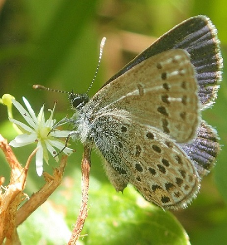
Distribution of Cranberry Blue Butterflies (Agriades optilete) and Their Responses to Forest Disturbance from In Situ Oil Sands and Wildfires

Department of Renewable Resources, Faculty of Agriculture, Life, and Environmental Sciences, University of Alberta, Edmonton, AB T6G 2H1, Canada
*
Author to whom correspondence should be addressed.
Diversity 2018, 10(4), 112; https://doi.org/10.3390/d10040112
Submission received: 26 September 2018 / Revised: 15 October 2018 / Accepted: 15 October 2018 / Published: 17 October 2018
(This article belongs to the Special Issue Butterfly Conservation)

Abstract

:
Cranberry blues (Agriades optilete) are butterflies of conservation interest worldwide. Less than 20 populations are known in Alberta, Canada, mostly inhabiting boreal forests that are increasingly fragmented by oil sands developments and subject to wildfires. We modeled the abundance of cranberry blues in the boreal forests of Alberta’s Wood Buffalo Region as a function of forest characteristics, presence of disturbances associated with in situ oil sands exploration, and wildfire disturbance, while accounting for butterfly detectability as a function of sampling conditions. We counted 188 cranberry blues during 1280 samples, discovering 14 unknown populations using a species distribution model based on forest wetness and canopy height. Probability of detection peaked around 5th July, and at higher temperatures and in the absence of wind, with cranberry blues preferring wetter treed peatland forests with low canopy heights. Seismic lines were positively related to the abundance of cranberry blues (400% increase), while exploratory well pads and wildfires were negatively related (60% and 90% loss, respectively). Overall, cranberry blue populations are small and locally sensitive to both natural and anthropogenic disturbances. Despite a narrow habitat specificity, cranberry blues seem more widely distributed than previously thought in northern Alberta (57% of the study area deemed suitable).

Graphical Abstract

1. Introduction

Anthropogenic variation in habitat amount, quality, and configuration affects the distribution and abundance of species worldwide [1,2,3,4,5,6], with evidence of declines in biodiversity emerging across a variety of taxa and environments [1,3,7,8,9,10]. Responses to habitat loss and fragmentation, pollution, and climatic change depend on species-specific ecological traits, with idiosyncrasies in magnitude and direction of effects [3,4,5,11,12]. The status of sensitive, “specialist” species, however, has been of particular concern [3,10,13]. Insects, including butterflies, mostly appear to be declining in the face of anthropogenic disturbances [1,8,10,13,14], and while some butterfly populations are indeed expanding [15,16], others are shrinking [13,17,18,19]. Lycaenids are among the most sensitive butterflies, including approximately one quarter of the European and one third of the North American butterflies on the “Red List” [20,21] due to localized populations, sensitivity to habitat quality, dispersal capacity, or obligate myrmecophilous associations [22,23,24]. One lycaenid of conservation interest is the cranberry blue, Agriades optilete (Figure 1).
In spite of its Holarctic distribution, cranberry blue populations are poorly known in Canada [25], seem sensitive to forest disturbance [16,26], and are expected to suffer the effects of climate change [6]. Cranberry blues are considered “imperiled” in Alberta [27], with less than 20 populations known [25]. Information on this species’ ecology is scarce and there are concerns that these few populations, generally inhabiting boreal treed peatlands [25], will be negatively affected by increasing natural and anthropogenic disturbances. Extraction of oil sands affects large areas of the Alberta boreal biome [16,28], while wildfires in these forests are becoming more frequent and severe [29], yet it is unknown which specific conditions and sites cranberry blues inhabit, and how this species responds to these different sources of forest disturbance.
Alberta’s boreal forests are “dissected” (sensu Jaeger [30]) across thousands of km2 by localized forest disturbances created during the location and extraction of a 142,000 km2 oil sands reserve. Because this reserve lies too deep for surface mining, oil extraction is performed with “in situ” techniques, using wells to reach the underground oil [12,31]. The most prevalent types of disturbances associated with in situ extraction are seismic lines (corridors cleared of trees and shrubs to facilitate seismic mapping of the underground reserve), and well pads (forest patches cleared to drill wells for exploration or extraction of oil sands). Seismic lines are narrow (usually <10 m) and widespread (up to 40 km/km2), while well pads are localized, rectangular clearings (usually 0.36–1 ha in the case of exploratory wells) [12,31]. While current best-management practices aim to reduce seismic line width (<5 m) [31], a legacy of wider (~10 m wide) corridors persist on the landscape after decades of their development [28], affecting forest structure and abiotic conditions [32], and in turn the distribution and behavior of organisms [12,31,33]. In previous studies of this system we found that butterfly diversity increased on well pads and 9-m wide lines, but not in 3-m wide, “low-impact”, lines when compared to reference undisturbed forests [16]. Both seismic line widths also conditioned the movement of a generalist butterfly [32].
Wildfire frequency is also increasing substantially in boreal forests, in part due to climate change [29], and while the effects of climate change on butterfly populations depend on the species’ ecology [13,15], increased frequency of extreme weather conditions are generally harmful [13]. Regardless, the boreal wildfire regime is necessary to maintain the spatial and temporal heterogeneity typical of this biome [33,34], yet responses to increases in frequency and severity of wildfire are difficult to predict, and may be negative even for boreal species that have evolved within this disturbance regime [33]. In 2016, approximately 6000 km2 of boreal forests burned (Figure 1) near Fort McMurray, Alberta, Canada [35], affecting a vast section of the boreal biome that could host cranberry blue populations. Cranberry blue is considered one of the least mobile butterflies in Canada [23] and depends on treed peatland habitats, which are particularly sensitive to wildfire disturbance [29]. Since insects generally suffer sharp population declines immediately after severe wildfires [36,37], wildfires could severely impact populations of cranberry blue, with these negative effects aggravated by cranberry blues’ limited mobility.
In 2015, while investigating the effects of in situ oil sands disturbances on butterflies [16], we discovered a population of cranberry blues. Unlike most butterfly species found in this area, cranberry blues were associated with undisturbed forests and avoided well pads and gravel roads. Given the rarity and sensitivity of cranberry blues, and because they rely on treed peatlands that are sensitive to both in situ oil sands developments and wildfires [28,29], we designed a series of follow-up studies to better understand this species’ ecology.
Specifically, we asked the following three questions:
(1)
Which forest types do cranberry blues inhabit?
(2)
What are the optimal conditions for observing cranberry blues?
(3)
How do cranberry blues respond to anthropogenic (i.e., clearing associated with in situ oil sands operations) and natural (i.e., wildfires) disturbance?
We hypothesized that cranberry blue prefers treed bogs and fens, i.e., “wet” peatland forests with short canopy heights [25], and that the narrow seismic line disturbances do not pose a threat to this species, while larger disturbances of well pads and severe wildfires negatively affect cranberry blue abundance [16,26,36,37].

2. Materials and Methods

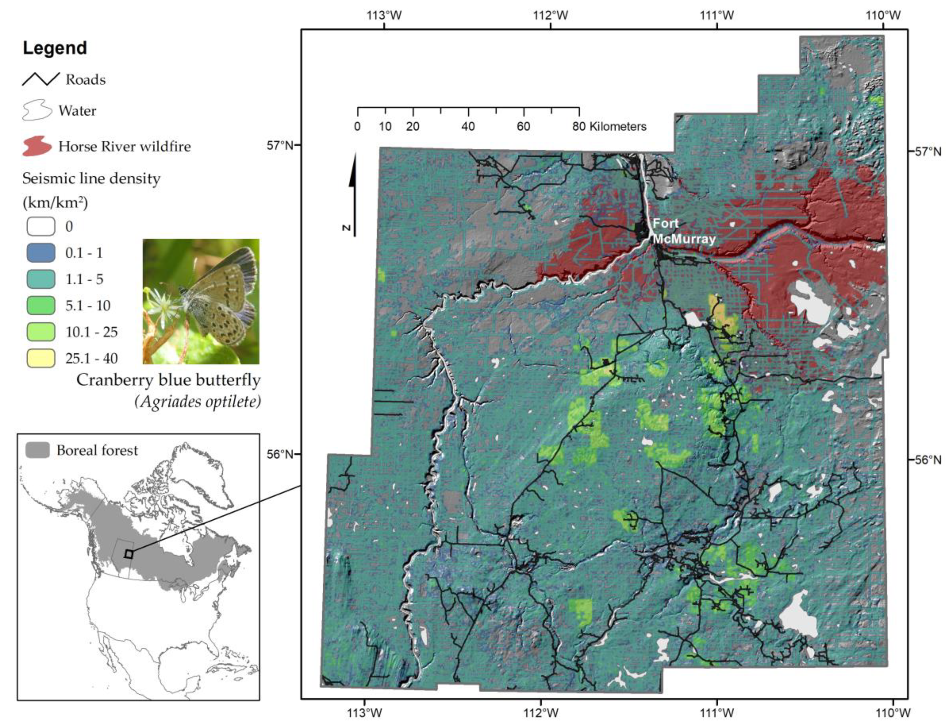
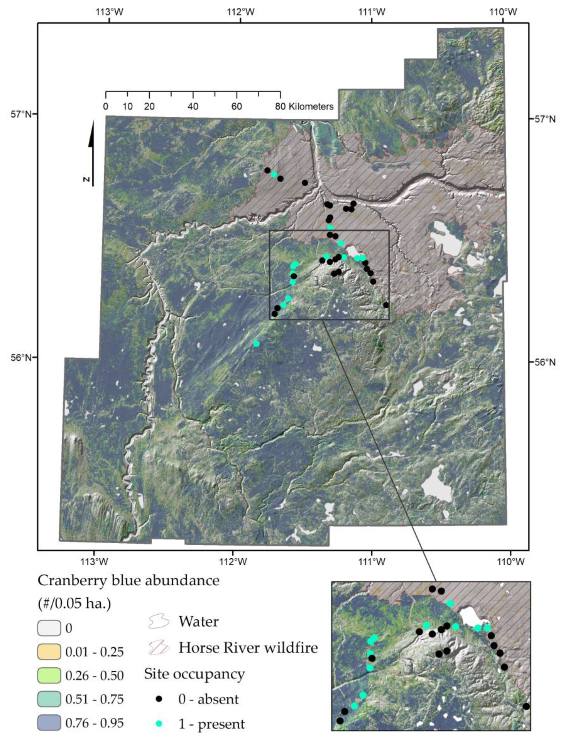
2.1. Study Area and Experimental Design

We conducted this research in the boreal forests of the Wood Buffalo region of northeast Alberta, Canada (Figure 1). There, forests are (i) heterogeneous, transitioning over short distances from wet, treed peatlands to drier, upland mixedwood forests; (ii) dissected by anthropogenic disturbances associated with oil sands exploration [16]; and (iii) extensively burned (approximately 6000 km2 of forests) during the 2016 Fort McMurray Horse River Wildfire [35]. We focused on treed peatlands dominated by black spruce (Picea mariana) and eastern larch (Larix laricina) which were hypothesized to provide suitable habitat for cranberry blues, but to further confirm this we also sampled a number of aspen (Populus tremuloides) mixedwood forest stands to verify that cranberry blues were not present in these forest types. We conducted two studies in the summers of 2016 and 2017 to identify which forests were inhabited by cranberry blues, and how this species responded to in situ oil sands exploration and wildfires. While the two studies differ in objectives and experimental design, in both studies we assessed boreal forest suitability for cranberry blues by stratifying sampling sites across different forest characteristics, using a Geographic Information System (GIS). We aimed to use indirect gradients to characterize the fundamental niche of cranberry blue in a “Grinnellian” fashion [38], creating a species distribution model across ~40,000 km2 of the Alberta Wood Buffalo region where anthropogenic disturbance associated with oil sands extraction is widespread (Figure 1).

2.2. Statistical Design and Sampling Conditions

Since traditional landcover data did not predict well the local abundance of cranberry blues, we used forest wetness and canopy height measured with Light Detection and Ranging (“LiDAR”, [39]) to describe more local variation in these boreal forest environments. We chose wetness and canopy height because they were potentially biologically meaningful (cranberry blues are found in bogs and fens characterized by a short coniferous canopy [16,25]) and because in this area they represent accurately the variation in forest characteristics [38]. Specifically, we used: (i) a distance-decay transformation of the depth-to-water index [40,41] (e−α×Depth-to-Water, with α = 4) as a measure of forest “wetness”, with wetness = 1 (depth-to-water = 0) indicating water at or near the surface in the whole raster cell, and (ii) a canopy height index ranging from 0 to 1, with all forests on average shorter than 5 m or taller than maximum tree height considered equal to 0 and 1 respectively. We transformed the depth-to-water index to minimize the effect of greater depths to water with many forests in the study area characterized by low depth-to-water, i.e., soils saturated in water for most of the year (50% quantile of the dept-to-water raster in the area = 0.03). Cranberry blues were sensitive to even subtle variation in forest wetness, and thus the distance-decay transformation better represented these slight variations. We also assumed that the effect of canopy height did not change at heights lower than 5 m. Statistical models included depth-to-water, canopy height, and their interaction. We did not observe high collinearity between wetness and canopy height (Pearson’s r = −0.59), although these relationships are known to occur [42]. Samples represented the number of cranberry blues observed at a point-count location (notice that sampling area and design differed between the two studies), and were modeled as counts assuming a Poisson distribution. All samples were conducted within controlled conditions following standard protocols (i.e., between 10 a.m. and 5 p.m., at temperature ≥17 °C, and wind speed <24 km/h (Beaufort scale ≤5)) to maximize detection rate [43,44]. While it is commonly assumed that variation in butterfly activity (detection) within this ranges is negligible, here we tested this assumption by quantifying how detection probability changes within these limits.

2.3. Responses to In Situ Oil Sands Disturbances

In 2016 (“oil sands study”) we focused on a ~30 km2 landscape in which we had previously located a population of cranberry blues [16], assessing at a local scale how forest wetness and canopy height determine the suitability of these forests for cranberry blues, and how different anthropogenic disturbance types affect abundance of cranberry blue butterflies. We stratified 120 sample sites on gradients of forest wetness and canopy height, and in four disturbance categories: control forests, 3-m wide (“low-impact”) seismic lines, 9-m wide (“conventional”) lines, and well pads, with 30 sample sites per category. Seismic lines and exploratory well pads had been cleared of trees and shrubs approximately 15 years before the study, resulting in early seral forests (i.e., disturbances were vegetated, but free of trees). No wildfires occurred in this area over the past 80 years, such that these anthropogenic clearings provide the only early seral sites in the 2016 study area. At each site we performed four point-counts (N = 480 samples) between 30th June and 16th July (supposed flight window in Alberta: 1st–30th July [25]), for three minutes/point, counting cranberry blues for each point-count in an area of 20 m2. While the general locations (i.e., the raster cell) where we conducted point-count samples were previously stratified in a GIS, point-counts were set in the field near microhabitats that seemed ideal to observe cranberry blues (e.g., ephemeral pools) within that raster cell. Therefore we chose a limited area of sampling to minimize the detection bias between forests and disturbances (and thus assume that different treatments did not affect probability of detecting cranberry blues), but increased the likelihood of observing cranberry blues by targeting micro-habitats deemed attractive for this species [16].

2.4. Responses to Wildfire and Distribution

Based on data collected in the 2016 study, we created a species distribution model for the Wood Buffalo Region, and designed a follow-up study in 2017 that concentrated on the effects of wildfire (“wildfire study”). We searched for unknown populations of cranberry blues across a larger landscape of ~10,000 km2, while assessing the response to severe wildfires, one year after disturbance. We visited 40 stratified sites each with a 250 m transect of five point-counts set every 50 m (200 total sample locations). Sites were set in seismic lines at early stages of forest succession and at a minimum distance of 1500 m apart to ensure independence among transects. We chose to set the point-counts in seismic lines because in 2016 we documented positive responses of cranberry blues to these disturbances, increasing our chances to detect new populations, and because it allowed us to access forests otherwise unreachable. To assess the effects of fire, 18 sites were set in forests severely burned during the 2016 Fort McMurray Horse River Wildfire (average tree mortality >85%). The 40 sites were selected in a GIS to represent a gradient of habitat suitability based on the results of part 1 (Supplementary Material). Sites were sampled twice between 22nd June and 15th July (because our first study suggested an earlier phenology then previously reported), for 15 min/transect, with two operators (FR and assistant) independently recording the number of cranberry blues observed in an area of ~500 m2 per point-count (N = 800 samples). Noticeably, while we sampled a larger area than in the oil sands study, i.e., five 50 × 10 m patches of early seral forests on each seismic line, these samples did not specifically target suitable microhabitat like those of the first study.

2.5. Statistical Analysis

We ran hierarchical Bayesian models using the package hSDM in R 3.4.3 [45]. We used a N-mixture model to predict the abundance of cranberry blues at each point-count location based on habitat suitability, spatial dependence between samples, and accounting for species detectability [46,47]. While habitat suitability is usually the main focus in species distribution models, ignoring spatial correlation and imperfect detection can lead to biased conclusions about ecological relationships [48,49,50,51]. We used this model because detection of cranberry blues varied within the sampling period, and point-count locations were closely spaced. Specifically, cranberry blue abundance (number of butterflies Ni; count response) is estimated as a function of habitat suitability, assuming a Poisson distribution, employing a Gaussian intrinsic conditional autoregressive (iCAR) model to capture spatial autocorrelation in the abundance of cranberry blues, while accounting for probability of detection assuming a Binomial distribution:
Habitat suitability process:
Ni ~ Poisson(λi)
log(λi) = Xi * β + ρi
Ni: Population size; Xi: Covariates explaining habitat suitability; ρi: spatial random effect.
Spatial autocorrelation:
ρi ~ Normal(μi, Vρ/ni)
μi: mean of ρi’ in the neighborhood; Vρ: variance of the spatial random effects; ni: number of neighbors.
Detectability process:
yit ~ Binomial(Ni, δit)
logit(δit) = Wit * γ
yit: Individuals counted at a location; δit: detection probability, t visits; Wit: Covariates explaining detection process.
We assumed that population density at a point-count location Ni did not change during the sampling period, with cranberry blues present either as eggs, larvae, pupae, or flying adults depending on the sampling day and individual variation in phenology (i.e., pupal eclosion date). Since we counted only cranberry blue adults (flying butterflies) in which abundance follows a unimodal distribution during the flight season (depending on pupae eclosion rate and adults mortality [51]), detection probability changed with time, and ordinal day was used as covariate in the detection process fitting a quadratic term. Note that the model does not account for butterfly death and replacement by newly-eclosed individuals over the sampling period, thus it underestimates the total abundance of cranberry blues. Assuming that mortality and eclosion rate do not vary between treatments, we can still use this model to compare relative abundance in different forest environments. Based on the preferred flying conditions for butterflies [44], we also included temperature (°C) in the detection process, hypothesizing a positive effect on detection probability, as well as a negative effect on detectability with increasing wind speed (km/h, classified following the Beaufort scale: 0 = 0 km/h; 1 = <4 km/h; 2 = 4–7 km/h; 3 = 8–12 km/h; 4 = 13–18 km/h; 5 = 19–24 km/h). Hour of the day was recorded during sampling but omitted from the final model due to poor fit, while an observer effect was included in part 2 to account for a potential bias in detection ability between the two observers (FR and assistant) in 2017.
Habitat suitability was estimated on the basis of: (i) forest wetness, canopy height, and their interactive term; (ii) anthropogenic disturbance categories (i.e., presence of well pad, low-impact line or conventional line vs. undisturbed forests); and (iii) wildfire disturbance (i.e., forests burned during the 2016 Fort McMurray Horse River Wildfire vs. forests that did not burn for at least 30 years). Posterior estimates of β coefficients refer to the average abundance of cranberry blues per point-count λi (which is not, but is relevant to, the distribution of the maximum abundance Ni given that Ni ~ Poisson(λi)). To assess the dependence between abundance of cranberry blues at neighbor sites we chose 300 m as a neighborhood distance, based on the dispersal capacities of other similar lycaenidae, and the low mobility of cranberry blues [23,37]. The intrinsic conditional autoregressive component of the model controls for spatial autocorrelation in the oil sands study (120 sites at a minimum distance of 50 m within the same landscape), while we used it as a “site” effect in the wildfire study (40 independent sites, i.e., 1.5 km or more from the other sites, composed by five “neighbor” point-count locations). Sensitivity analysis at neighborhood distances of 100 m and 500 m returned analogous results.
Continuous covariates were standardized by subtracting the mean and dividing by the standard deviation. Model parameters were estimated using a Gibbs sampler through an adaptive Metropolis algorithm, and the parameters’ conditional posterior distributions were assessed after 150,000 iterations, using a burn-in of 140,000 iterations and a thinning rate of 25 (400 posterior samples retained for analysis). We presented each parameter posterior mean and the 95% Highest Posterior Density (HPD) intervals (i.e., interval between 2.5% and 97.5% quantiles of posterior samples). Models were run using uninformative priors for the oil sands study, and using the posterior estimates of the oil sands study as priors for the wildfire study (only for covariates shared between the two, assuming equal mean and standard deviation of covariates between the two field seasons; intercepts were set with uninformative priors given different sampling efforts). Posterior estimates of parameters for the wildfire study were similar with informative and uninformative priors, with no change in estimated direction of effects. Given the normal distribution of the posterior samples (Supplementary Material), we calculated the probability p that a model parameter was equal to zero or opposed in sign to the mean posterior estimate by integrating the parameter normal distribution based on the posterior mean and standard deviation of each parameter, and comparing the areas before/after zero. Similarly, the 95% credible intervals of λi and δi (i.e., interval between 2.5% and 97.5% quantiles of predicted values) were obtained by simulating 100,000 times the linear predictors (i.e., log(λi) = Xi * β and logit(δit) = Wit * γ) generating random βs and γs from normal distributions described by the posterior estimates of each parameter mean and standard deviation.
Finally, cranberry blue average abundance (λi) was predicted for each raster cell in the study area to generate a distribution-abundance model based on forest wetness, canopy height, their interactive term, and the effects of wildfire disturbance (2016 Horse River Wildfire). We used the β estimated in part 2, ignoring the spatial component of the model ρ (losing the positive or negative effect associated with the random effect of each spatial entity), but maintaining the relative effect of the habitat covariates on cranberry blue abundance. Notice that these values refer to 500 m2 point-counts conducted in 3 min in seismic lines.

3. Results

We observed 64 cranberry blues during 480 point-counts in the 2016 oil sands study, and 124 cranberry blues during 800 point-counts in the 2017 wildfire study (Table 1).
Assessing the effects of in situ oil sands exploration, we observed 16 cranberry blues in forests vs. 12 in low-impact seismic lines, 33 in conventional seismic lines, and 3 in well pads, from 37 of the 120 point-count locations sampled (Table 1). Assessing the effects of wildfires, we observed 115 cranberry blues in unburned forests, from 34 point-count locations in 11 sites, and 9 cranberry blues in burned forests one year after disturbance, from 6 point-count locations in 3 sites (Table 1). Posterior estimates of the effect of covariates on detection (γ) and abundance (β) of cranberry blues are shown in Figure 2 and Table A1 (Appendix A), while probability of detection and predicted abundance at each point-count location are shown in Figure 3.

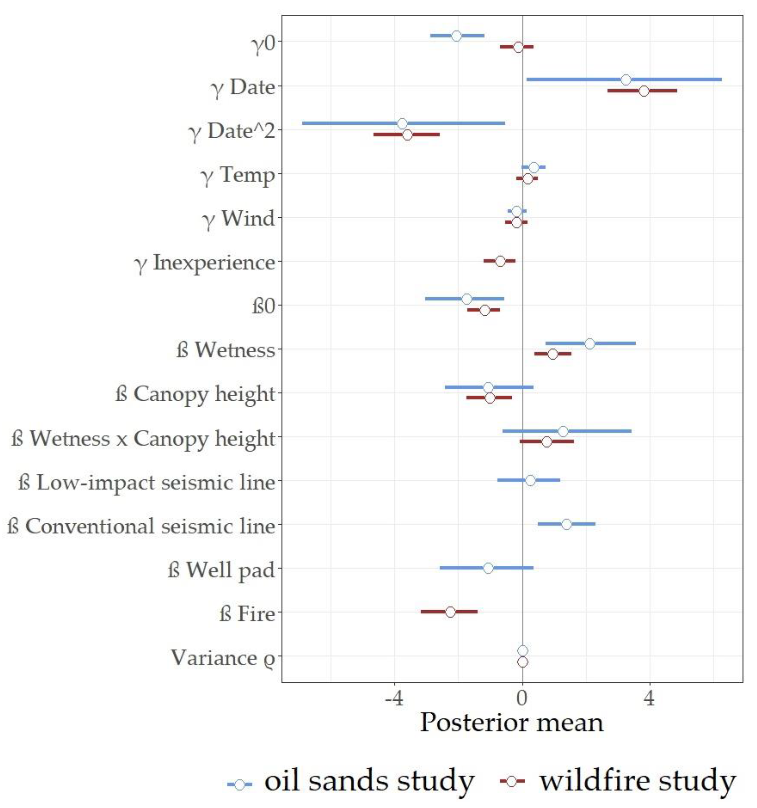
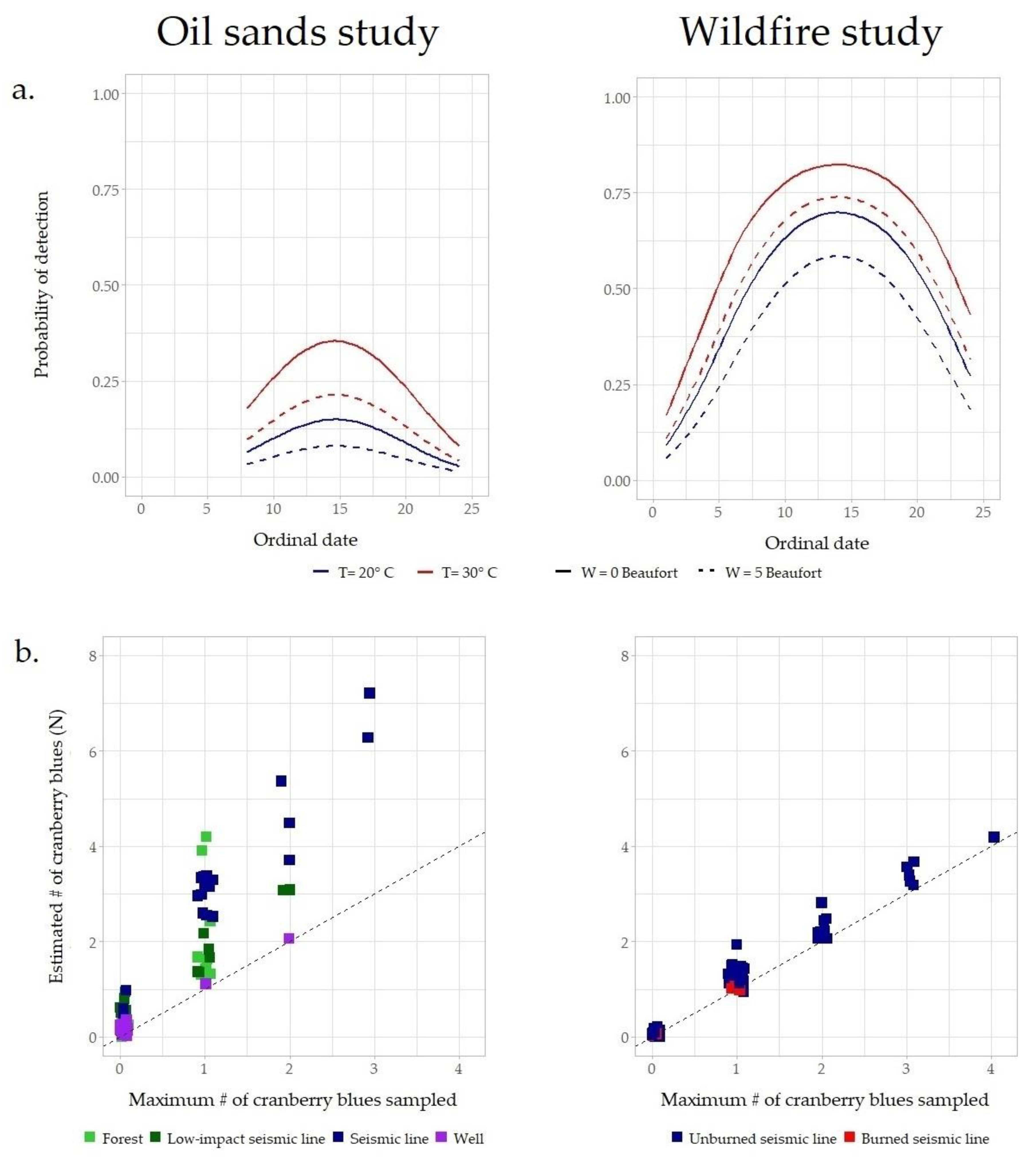
3.1. Probability of Detection of Cranberry Blues

Posterior mean detection probability (p) for FR was 11.4% (C.I: 5.2%–23%) in the oil sands study, and 46.7% (C.I: 34%–59.8%) in the wildfire study, while an unexperienced assistant had 30.5% (C.I: 17.6%–47.5%) mean probability of detection of cranberry blues in the wildfire study. Cranberry blues are more-easily observed at higher temperatures, lower wind speeds, and during the first two weeks of July (Figure 3). Around 5th July, at a temperature of 30 °C and an absence of wind, the estimated probability of detection reaches 34.9% (C.I: 3.7%–88%) in the oil sands study and 79.8% (C.I: 56.9%–92.2%) in the wildfire study. At a temperature of 20 °C and wind speed of ~20 km/h, probability of detection decreased to 8.1% (C.I: 1%–58.8%) in the oil sands study, and to 55.6% (C.I: 32.5%–76.5%) in the wildfire study.

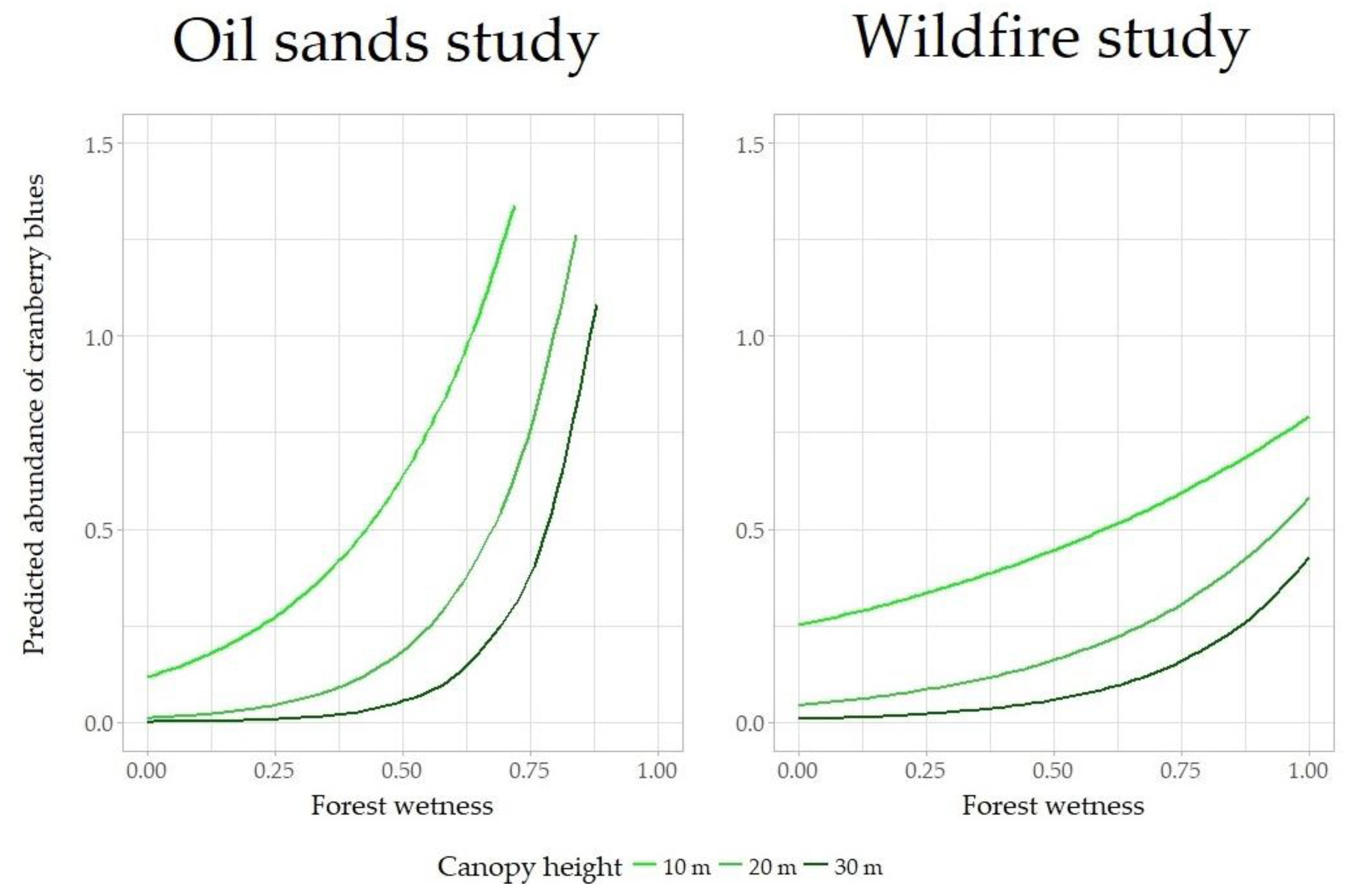
3.2. Abundance of Cranberry Blues

Posterior mean abundance (λ) was 0.17 cranberry blues per point-count sample (C.I: 0.05–0.60) in the oil sands study, and 0.31 cranberry blues per point-count sample (C.I: 0.19–0.50) in the wildfire study. Posterior mean variance associated to the spatial random effect ρ was ~0 in both part studies. Abundance of cranberry blues increased with forest wetness, decreased with canopy height, and increased with their interactive term (Figure 4). For instance, in wet forests (wetness = 0.8) with canopy heights of 10, 20, and 30 m, the model estimates in the oil sands study had a posterior mean abundance of 2.11 (C.I: 0.33–13.4), 1.37 (C.I: 0.27–6.87), and 0.88 (C.I: 0.11–6.84) cranberry blues per point-count sample in seismic lines, and in the wildfire study a posterior mean abundance of 0.67 (C.I: 0.33–1.35), 0.40 (C.I: 0.23–0.68), and 0.23 (C.I: 0.10–0.53) cranberry blues per point-count sample in seismic lines.
After accounting for forest characteristics, abundance was similar between control forests and low-impact seismic lines, increased in conventional seismic lines, and decreased with well pads and after the 2016 Horse River Wildfire (Figure 3b and Table A1). Assuming forest wetness = 0.8 and canopy height = 10 m, the model based on the oil sands study predicts an average of 0.53 cranberry blues per point-count sample (C.I.: 0.10–2.75) in undisturbed forests vs. 0.69 in low-impact lines (C.I.: 0.10–4.60), 2.11 per point-count sample in conventional seismic lines (C.I.: 0.33–13.5), and 0.19 per point-count sample in well pads (C.I.: 0.02–1.17). With analogous forest conditions, the model based on the wildfire study predicts 0.67 cranberry blues per point-count sample (C.I.: 0.33–1.35) in unburned seismic lines vs. 0.07 (C.I.: 0.02–0.22) per point-count sample in burned seismic lines (Figure 2 and Figure 3). The 14 cranberry blues populations were observed in forests that, based on the results of the oil sands study, have a predicted average abundance of cranberry blues per point-count sample (λ) >0.4, in approximately 56% of the sites suitable based on our results (Supplementary Material). Predicted average abundance of cranberry blues per point-count sample across the landscape based on the wildfire study is shown in Figure 5.

4. Discussion

This study investigated distribution, abundance, phenology, behavior, and responses to disturbance of habitat for cranberry blue butterflies (Agriades optilete), focusing on populations inhabiting the Alberta Wood Buffalo Region (Figure 1). We had three objectives: (i) assess responses to the different types of disturbance occurring in this area (i.e., anthropogenic disturbance associated with widespread in situ oil sand assessments, and natural disturbance due to wildfires); (ii) assess how abundance and distribution are affected by natural variation in wetness and canopy height; and (iii) clarify the flight period of these populations.
Cranberry blues were uncommon, with only 188 cranberry blues recorded in 1280 surveys across two field seasons. Yet, our results suggest that these butterflies are not as rare across the landscape as previously hypothesized (more than 50% of suitable sites occupied). Among many forms of rarity, therefore, it seems like cranberry blue belong to those species having a large geographic range, but a narrow habitat specificity and small local populations [52]. While less than 20 populations were previously known in Alberta [25], we discovered 14 new populations from ~25 sites deemed suitable based on a preliminary distribution model (Figure 5; Supplementary Material). Since an important portion of the area represents suitable forests (Figure 5), i.e., treed peatland forests with short canopies, cranberry blues could be relatively widely distributed in the Wood Buffalo Region. Indeed, 57% of the raster is predicted to be suitable habitat for cranberry blues, most broadly defined as treed peatlands. Still, cranberry blues were low in number in any occupied sites.
Further studies are necessary to estimate with more accuracy this species’ abundance in the Wood Buffalo Region, particularly because we lack data on mortality and eclosion rates for these populations [51]. Many factors hinder an estimation of the number of cranberry blues inhabiting the Wood Buffalo Region. First, the model assumption of a closed population is broken by butterflies, with individuals that died and were replaced by eclosing pupae during the sampling period. Then, differences in sampling design between seasons are hard to interpret because, while there could be differences between abundance of cranberry blues between 2016 and 2017, the two sampling designs differ in quality and quantity of area sampled. It was surprising that, despite a 25-times smaller area sampled, the estimated abundance of cranberry blues in seismic lines was slightly higher in the oil sands study (Figure 3). Yet, in our first study the point-count location where set in areas deemed optimal to observe cranberry blues, while in our second study the larger sampling area often included less-suitable sites. Cranberry blues seemed to depend on highly localized conditions, and were particularly stationary near small pools of water that we targeted in our first study (especially territorial males). As well, the lower probability of detection in the oil sands study could also have affected model estimates. Despite these limitations, the relationship between the abundance of cranberry blues and forest wetness and canopy height was consistent between our studies, suggesting that most of the peatland forests in the area are suitable for cranberry blues.
As previously reported [25], cranberry blues preferred boreal peatland forests (bogs and fens), here identified using forest wetness and canopy height measured with LiDAR. The effects of wetness and canopy height were consistent with expectations in both studies, while an interaction term between forest wetness and canopy height had a stronger effect in the oil sands study (Figure 4). Even though we assessed the effects of forest wetness and canopy height in both studies, to maximize our chances of discovering new populations we sampled only seismic lines in the wildfire study, because in the oil sands study cranberry blues were observed more frequently in these narrow early seral corridors. Seismic lines affect hydrology and canopy height at local scales (higher wetness, canopy removed [31]), and the 50 × 50 m raster cell used to describe habitat suitability diminished these effects. Therefore, we believe that the most likely relationship between forest wetness, canopy height, and cranberry blue abundance is that observed in the oil sands study, with cranberry blues mostly occurring in short forests (canopy height <20 m) with soils saturated in water for most of the year (Wetness >0.7). While any value of wetness >0.7 represents a wet environment, it appears that this species prefers environments where the peat is saturated with water, if not submerged (Wetness ~1, i.e., depth-to-water = 0). The canopy is low and open in these forests, usually with only a few, short, black spruce trees (Picea mariana) able to establish.
Cranberry blue caterpillars are thought to feed on Vaccinium spp., but the Low Bilberry (V. myrtillus) on which larvae are known to feed in North America are not present in Alberta’s boreal forests [25]. Yet, other Vaccinium spp. are among the early seral species that increase when the canopy is more open in boreal forests [53]. V. myrtilloides was observed in drier (unsuitable) upland conditions, and is thus unlikely to be the larval host plant in these forests. Bog cranberry or small bog cranberry (V. oxycoccos and V. vitis-idaea) are common in treed peatlands, yet we did not observe any correlation with these species and cranberry blues. Given that these plants were fairly common, particularly V. vitis-idaea, other factors likely limit the distribution of cranberry blues in these environments. We speculate that abiotic conditions (e.g., temperature, humidity) may play an important role, but future studies at local scales will be necessary to reveal the mechanisms underlying the differences in abundance of cranberry blues. One factor that potentially is increasing local abundance of cranberry blues (or their behavior) was higher availability of nectar sources on seismic lines. Seismic lines have higher plant diversity than adjacent forests [31] with noticeable lower floral resources in typical undisturbed peatland forests. However, we rarely observed cranberry blue nectaring during our study beyond a few individuals on small, white flowers such as chickweed (Stellaria longifolia) or bog cranberry (V. oxycoccos) flowers. Ultimately, cranberry blues seemed more related to the overall surrounding forest conditions than to the availability of larval host plants or nectar sources. Some lycaenids are known to have territorial behaviors such as perching on locations deemed attractive for mating [22]. Seismic lines might simply represent attractive sites for this behaviour, with males often observed in proximity of superficial water pools.
Knowing when and at which conditions species are more-easily detected is important when planning sampling designs and monitoring protocols [50]. We showed that cranberry blue populations in northeast Alberta fly approximately between 20th June and 20th July, with the highest probability of detection during the first ten days of July. Changes in detectability with all covariates were similar between 2016 and 2017, despite different probabilities of detection between field seasons due to different sampling designs (Figure 3; this is not surprising, since the area assessed in 2017 was ~25 times larger than the area assessed in 2016). Ordinal day was the most important covariate in explaining probability of detection of cranberry blues, with a shorter and earlier flight period than previously reported [25]. The effects of temperature (positive) and wind (negative) were consistent with our expectations, while the effect of time of day was not included in the final model because it was highly variable. Interestingly, despite conducting our point-counts during standard sampling conditions, the posterior average probability of detection varied by ~20% at the flight curve peak depending on temperature and wind conditions (Figure 3). These results suggest that the common assumption of equal detectability within standard environmental conditions (i.e., between 10 a.m. and 5 p.m., at temperature >17 °C, winds at Beaufort scale <5 [43,44]) may not always be met. Therefore, when possible, we recommend accounting for variation in detection probability due to sampling conditions in analyzing butterfly data obtained from repeated surveys of the same site (e.g., common monitoring protocols such as Pollard transects or point-counts [51]). Finally, the only other lycaenids that inhabit these environments at the end of June and beginning of July are dorcas coppers (Lycaena dorcas). Dorcas coppers are easily distinguishable from cranberry blues given pronounced color differences (i.e., golden and purple colors vs. silver and blue, respectively). In conclusion, we believe that our results represent the actual abundance of the target species, and not our inability to detect it or the confusion with other lycaenids.
Responses to disturbance differed in the direction and magnitude of effects depending on the disturbance type. Despite concerns regarding the density of seismic lines in the Wood Buffalo Region [12,31,32], our study confirms preliminary findings that cranberry blues—like most other butterflies—responded positively to seismic line corridors (4-times more cranberry blues than in reference forests), with no effect of the narrower “low-impact” seismic lines [16]. Yet, differently from the other butterfly species inhabiting these forests [16], we documented negative responses to exploratory well pads, i.e., 60 × 60 m anthropogenic forest clearings associated with oil sands exploration (less than half the cranberry blues were seen here in comparison to analogous forests). Openings in the forest canopy, such as seismic lines, allow early seral plant species, on which butterflies rely for nectar sources and larval host plants, to increase in abundance and diversity [53], and thus seem to benefit the whole butterfly community [16]. On the other hand, both seismic lines and well pads affect abiotic conditions by increasing illuminance and wind speeds [54]. While abiotic conditions in seismic lines are more similar to those of undisturbed forests, the effects of well pads are more substantial, with 16-times higher average wind speed, 4-times higher maximum wind speed, and 3-times higher illuminance [54]. These conditions may negatively affect cranberry blues, particularly due to wind speed that may limit the movement of these small (~25 mm wingspan) butterflies. Another study conducted in European boreal forests documented similar, negative responses to large clear cuts [26]. Yet, given the positive relationship observed between the abundance of cranberry blues and conventional (9-m wide) seismic line corridors, some types of disturbance could provide the conditions necessary for this species to thrive. Indeed, while in situ oil sands developments have only recently appeared in these forests, wildfires have long characterized the boreal biome with most boreal species being adapted to this disturbance regime [33]. Here, we found that recent wildfire had a substantial negative effect on cranberry blue abundance in the short term, with our model predicting a loss of 90% of cranberry blues in burned forests one year after disturbance. This type of response has been observed commonly in other butterfly and insect taxa [36,37]. However, wildfires may be particularly threatening to cranberry blues because the frequency and severity of wildfires are predicted to increase, and peatlands are one of the most sensitive habitats in the boreal biome [29]. Limited adult dispersal between patches and specialization of larval habitats limit small populations in disturbed landscapes [13], and while the genus Vaccinium is one of the most common plant taxa in the Alberta boreal biome, dispersal of cranberry blue may be too slow to effectively re-colonize burned peatlands, which may in turn require time to return to suitable conditions for cranberry blues. Indeed, the common opinion that cranberry blue mobility is low [23] was confirmed by our first study, where the spatial component of our model explained little variation in the predicted abundance of cranberry blues (Supplementary Material). On the other hand, follow-up studies will be necessary to reveal the number of years required post-fire before treed peatlands can support abundant cranberry blue populations.
Finally, while preliminary analyses with landcover data did not successfully predict cranberry blue abundance, forest wetness and canopy height did predict this species’ abundance, confirming that LiDAR data can be a valuable resource for conservation purposes (e.g., [39]). Note that we did not include climate variables and elevation in our analysis assuming secondary effects at this more regional scale (Figure 1). Future studies aiming to assess the distribution of cranberry blues at larger scales should account for potential effects on phenology and distribution of these factors.

5. Conclusions

This study was a first step toward documenting the ecology of cranberry blues in northeastern Alberta and assessing their conservation status. We described the relationships between cranberry blue abundance, forest characteristics, and natural and anthropogenic disturbances. Cranberry blues were not abundant, and most common in wet forests with low canopies, and on seismic lines. In contrast, cranberry blue abundance was substantially lower in well pads and burned forests. While our results suggest that cranberry blues are more common than previously hypothesized in this region (we doubled the number of known populations in Alberta), we stress that this species’ populations are generally scarce, and that both anthropogenic and natural disturbance will increase in these forests [12,29]. Not only will wildfires increase with climate change [29], but models also suggest that they will mediate a change in vegetation toward less-suitable upland forests [55]. Therefore, future studies should monitor the status of cranberry blues in northeastern Alberta to determine if there are reasons for concern for this species. Based on our results, future studies should focus on the period between 1st–10th July, and collecting data at temperatures >25 °C with no wind.

Supplementary Materials

The following are available online at https://www.mdpi.com/1424-2818/10/4/112/s1, s1: Riva et al., cranberry blues responses to disturbance and distribution in northeastern Alberta—zip file containing data and R script for analysis.

Author Contributions

F.R., J.H.A. and S.E.N. conceived the study; F.R. designed the experiment, collected the data and performed the analyses; F.R. wrote the manuscript with assistance from J.H.A. and S.E.N.

Funding

The project was supported by Xerces Society via the Joan Mosenthal DeWind Award (RES0036460), COSIA (CRDPJ 498955), Alberta Innovates—Energy and Environmental Solutions (ABIEES 2070), Alberta Agriculture and Forestry (15GRFFM12), NSERC-CRD and the LRIGS NSERC-CREATE programme (CRD 498955-16, CREATE 397892), and Alberta Conservation Association via the ACA Grants in Biodiversity (RES0034641).

Acknowledgments

We thank Shawn Eckert, Fionnuala Carrol and Marcel Schneider for assisting in field, and Peter Blenis for support with ggplot2 and analysis.

Conflicts of Interest

The authors declare no conflict of interest. The funders had no role in the design of the study; in the collection, analyses, or interpretation of data; in the writing of the manuscript, and in the decision to publish the results.

Appendix A

Table A1. Posterior mean, standard deviation, 2.5% quantile, and 97.5% quantile of the effects of model covariates on cranberry blue detection (γ coefficients) and abundance (β coefficients), including a conditional autoregressive component to account for spatial autocorrelation in abundance of cranberry blues between sampling locations closer than 300 m (Variance ρ); p = probability that a posterior estimate is equal to zero or opposite in sign to the posterior mean.
Case-StudyCoefficientMeanStandard Deviation2.5% Quantile97.5% Quantilep
Oil sandsβ (Intercept)−1.730.64−3.03−0.55<0.01
Oil sandsβ well pad−1.050.76−2.580.370.08
Oil sandsβ low-impact line0.250.50−0.761.190.31
Oil sandsβ conventional line1.370.460.512.29<0.01
Oil sandsβ Wetness2.120.720.743.58<0.01
Oil sandsβ Canopy height−1.060.70−2.400.350.06
Oil sandsβ Wetness × Canopy height1.281.06−0.613.440.11
Oil sandsγ (Intercept)−2.050.43−2.88−1.17<0.01
Oil sandsγ Date3.231.560.166.260.02
Oil sandsγ Date^2−3.771.62−6.89−0.520.01
Oil sandsγ Temperature0.350.19−0.010.730.04
Oil sandsγ Wind−0.160.15−0.440.160.14
Oil sandsVariance ρ<0.01<0.01<0.01<0.010.04
Wildfireβ (Intercept)−1.170.26−1.70−0.70<0.01
Wildfireβ Wetness0.950.300.391.54<0.01
Wildfireβ Canopy height−1.020.37−1.74−0.32<0.01
Wildfireβ Wetness × Canopy height0.770.44−0.071.640.04
Wildfireβ Fire−2.240.45−3.16−1.38<0.01
Wildfireγ (Intercept)−0.130.27−0.680.370.31
Wildfireγ Date3.800.572.674.86<0.01
Wildfireγ Date^2−3.590.54−4.65−2.56<0.01
Wildfireγ Temperature0.170.17−0.170.500.16
Wildfireγ Wind−0.170.18−0.520.170.16
Wildfireγ Observer−0.700.26−1.20−0.20<0.01
WildfireVariance ρ<0.01<0.01<0.01<0.01<0.01

References

  1. Dirzo, R.; Young, H.S.; Galetti, M.; Ceballos, G.; Isaac, N.J.B.; Collen, B. Defaunation in the Anthropocene. Science 2014, 345, 401–406. [Google Scholar] [CrossRef] [PubMed] [Green Version]
  2. Haddad, N.M.; Brudvig, L.A.; Clobert, J.; Davies, K.F.; Gonzalez, A.; Holt, R.D.; Lovejoy, T.E.; Sexton, J.O.; Austin, M.P.; Collins, C.D.; et al. Habitat fragmentation and its lasting impact on Earth’s ecosystems. Sci. Adv. 2015, 1, e1500052. [Google Scholar] [CrossRef] [PubMed]
  3. Pfeifer, M.; Lefebvre, V.; Peres, C.A.; Banks-Leite, C.; Wearn, O.R.; Marsh, C.J.; Butchart, S.H.M.; Arroyo-Rodríguez, V.; Barlow, J.; Cerezo, A.; et al. Creation of forest edges has a global impact on forest vertebrates. Nature 2017, 551, 187–191. [Google Scholar] [CrossRef] [PubMed]
  4. Fahrig, L. Ecological Responses to Habitat Fragmentation Per Se. Annu. Rev. Ecol. Evol. Syst. 2017, 48, 1–23. [Google Scholar] [CrossRef]
  5. Tylianakis, J.M.; Didham, R.K.; Bascompte, J.; Wardle, D.A. Global change and species interactions in terrestrial ecosystems. Ecol. Lett. 2008, 11, 1351–1363. [Google Scholar] [CrossRef] [PubMed] [Green Version]
  6. Devictor, V.; Van Swaay, C.; Brereton, T.; Brotons, L.; Chamberlain, D.; Heliölö, J.; Herrando, S.; Julliard, R.; Kuussaari, M.; Lindström, Å.; et al. Differences in the climatic debts of birds and butterflies at a continental scale. Nat. Clim. Chang. 2012, 2, 121–124. [Google Scholar] [CrossRef] [Green Version]
  7. Hanski, I. Habitat fragmentation and species richness. J. Biogeogr. 2015, 42, 989–993. [Google Scholar] [CrossRef] [Green Version]
  8. Potts, S.G.; Biesmeijer, J.C.; Kremen, C.; Neumann, P.; Schweiger, O.; Kunin, W.E. Global pollinator declines: Trends, impacts and drivers. Trends Ecol. Evol. 2010, 25, 345–353. [Google Scholar] [CrossRef] [PubMed]
  9. Fletcher, R.J.; Didham, R.K.; Banks-leite, C.; Barlow, J.; Ewers, R.M.; Rosindell, J.; Holt, R.D.; Gonzalez, A.; Pardini, R.; Damschen, E.I.; et al. Is habitat fragmentation good for biodiversity? Biol. Conserv. 2018, 226, 9–15. [Google Scholar] [CrossRef]
  10. Martinson, H.M.; Fagan, W.F. Trophic disruption: A meta-analysis of how habitat fragmentation affects resource consumption in terrestrial arthropod systems. Ecol. Lett. 2014, 17, 1178–1189. [Google Scholar] [CrossRef] [PubMed]
  11. Haddad, N.M.; Hudgens, B.; Damschen, E.I.; Levey, D.J.; Orrock, J.L.; Tewksbury, J.J.; Weldon, A.J. Assessing positive and negative ecological effects of corridors. In Sources, Sinks and Sustainability; Liu, J., Hull, V., Morzillo, A.T., Wiens, J.A., Eds.; Cambridge University Press: Cambridge, UK, 2011; pp. 475–503. ISBN 9780511842399. [Google Scholar]
  12. Fisher, J.T.; Burton, A.C. Wildlife winners and losers in an oil sands landscape. Front. Ecol. Environ. 2018, 16, 323–328. [Google Scholar] [CrossRef]
  13. Thomas, J.A. Butterfly communities under threat. Science 2016, 353, 216–218. [Google Scholar] [CrossRef] [PubMed]
  14. Hallmann, C.A.; Sorg, M.; Jongejans, E.; Siepel, H.; Hofland, N.; Schwan, H.; Stenmans, W.; Müller, A.; Sumser, H.; Hörren, T.; et al. More than 75 percent decline over 27 years in total flying insect biomass in protected areas. PLoS ONE 2017. [Google Scholar] [CrossRef] [PubMed]
  15. Menéndez, R.; González-Megías, A.; Lewis, O.T.; Shaw, M.R.; Thomas, C.D. Escape from natural enemies during climate-driven range expansion: A case study. Ecol. Entomol. 2008, 33, 413–421. [Google Scholar] [CrossRef]
  16. Riva, F.; Acorn, J.H.; Nielsen, S.E. Localized disturbances from oil sands developments increase butterfly diversity and abundance in Alberta’s boreal forests. Biol. Conserv. 2018, 217, 173–180. [Google Scholar] [CrossRef]
  17. Swengel, S.R.; Schlicht, D.; Olsen, F.; Swengel, A.B. Declines of prairie butterflies in the midwestern USA. J. Insect Conserv. 2011, 15, 327–339. [Google Scholar] [CrossRef]
  18. Van Swaay, C.; Van Strien, A.; Harpke, A. The European Grassland Butterfly Indicator: 1990–2011; Lund University: Lund, Sweden, 2013. [Google Scholar]
  19. Sands, D.P.A.; New, T.R. Conservation of the Richmond Birdwing Butterfly in Australia; Springer: Dordrecht, The Netherlands, 2013; ISBN 9789400771703. [Google Scholar]
  20. Van Swaay, C.; Cuttelod, A.; Collins, S.; Maes, D.; López Munguira, M.; Šašić, M.; Settele, J.; Verovnik, R.; Verstrael, T.; Warren, M.; et al. European Red List of Butterfies; International Union for Conservation of Nature: Gland, Switzerland, 2010; ISBN 9789279141515. [Google Scholar]
  21. Xerces Society Red Listed butterflies of North America. Available online: https://xerces.org/red-lists/ (accessed on 16 October 2018).
  22. New, T.R. Conservation Biology of Lycaenidae (Butterflies); IUCN Species Survival Commission: Gland, Switzerland, 1993. [Google Scholar]
  23. Burke, R.J.; Fitzsimmons, J.M.; Kerr, J.T. A mobility index for Canadian butterfly species based on naturalists’ knowledge. Biodivers. Conserv. 2011, 20, 2273–2295. [Google Scholar] [CrossRef]
  24. Riva, F.; Barbero, F.; Bonelli, S.; Balletto, E.; Casacci, L.P. The acoustic repertoire of lycaenid butterfly larvae. Bioacoustics 2017, 26, 77–90. [Google Scholar] [CrossRef]
  25. Bird, C.D.; Hilchie, G.J.; Kondla, N.G.; Pike, E.M.; Sperling, F.A.H. Alberta Butterflies; Alberta Public Affairs Bureau/Queens Printer, The Provincial Museum of Alberta: Edmonton, AL, USA, 1995; ISBN 0-7732-1672-3. [Google Scholar]
  26. Viljur, M.L.; Teder, T. Butterflies take advantage of contemporary forestry: Clear-cuts as temporary grasslands. For. Ecol. Manag. 2016, 376, 118–125. [Google Scholar] [CrossRef]
  27. NatureServe Explorer: An Online Encyclopedia of Life [Web Application]. Version 7.1. 2017. Available online: http://www.natureserve.org/explorer (accessed on 16 October 2018).
  28. Van Rensen, C.K.; Nielsen, S.E.; White, B.; Vinge, T.; Lieffers, V.J. Natural regeneration of forest vegetation on legacy seismic lines in boreal habitats in Alberta’s oil sands region. Biol. Conserv. 2015, 184, 127–135. [Google Scholar] [CrossRef]
  29. Flannigan, M.D.; Krawchuk, M.A.; de Groot, W.J.; Wotton, M.B.; Gowman, L.M. Implications of changing climate for global wildland fire. Int. J. Wildl. Fire 2009, 18, 483–507. [Google Scholar] [CrossRef]
  30. Jaeger, J.A.G. Landscape division, splitting index, and effective mesh size: New measures of landscape fragmentation. Landsc. Ecol. 2000, 15, 115–130. [Google Scholar] [CrossRef]
  31. Dabros, A.; Pyper, M.; Castilla, G. Seismic lines in the boreal and arctic ecosystems of North America: Environmental impacts, challenges, and opportunities. Environ. Rev. 2018, 16, 1–16. [Google Scholar] [CrossRef]
  32. Riva, F.; Acorn, J.H.; Nielsen, S.E. Narrow anthropogenic corridors direct the movement of a generalist boreal butterfly. Biol. Lett. 2018. [Google Scholar] [CrossRef] [PubMed]
  33. Weber, M.G.; Stocks, B.J. Forest fires and sustainability in the boreal forests of Canada. Ambio 1998, 27, 545–550. [Google Scholar]
  34. Burton, P.J.; Parisien, M.A.; Hicke, J.A.; Hall, R.J.; Freeburn, J.T. Large fires as agents of ecological diversity in the North American boreal forest. Int. J. Wildl. Fire 2008, 17, 754–767. [Google Scholar] [CrossRef]
  35. Simms, C.D. Canada’s Fort McMurray fire: Mitigating global risks. Lancet Glob. Health 2016, 4, e520. [Google Scholar] [CrossRef]
  36. New, T.R. Insects, Fire and Conservation; Springer: Basel, Switzerland, 2014; ISBN 9783319080963. [Google Scholar]
  37. Swengel, A.B. A literature review of insect responses to fire, compared to other conservation managements of open habitat. Biodivers. Conserv. 2001, 10, 1141–1169. [Google Scholar] [CrossRef]
  38. Guisan, A.; Zimmermann, N.E. Predictive habitat distribution models in ecology. Ecol. Model. 2000, 135, 147–186. [Google Scholar] [CrossRef]
  39. Guo, X.; Coops, N.C.; Tompalski, P.; Nielsen, S.E.; Bater, C.W.; John Stadt, J. Regional mapping of vegetation structure for biodiversity monitoring using airborne lidar data. Ecol. Inform. 2017, 38, 50–61. [Google Scholar] [CrossRef]
  40. Oltean, G.S.; Comeau, P.G.; White, B. Linking the depth-to-water topographic index to soil moisture on boreal forest sites in Alberta. For. Sci. 2016, 62, 154–165. [Google Scholar] [CrossRef]
  41. Murphy, P.N.C.; Ogilvie, J.; Connor, K.; Arp, P.A. Mapping wetlands: A comparison of two different approaches for New Brunswick, Canada. Wetlands 2007, 27, 846–854. [Google Scholar] [CrossRef]
  42. Mao, L.; Bater, C.W.; Stadt, J.J.; White, B.; Tompalski, P.; Coops, N.C.; Nielsen, S.E. Environmental landscape determinants of maximum forest canopy height of boreal forests. J. Plant Ecol. 2017. [Google Scholar] [CrossRef]
  43. Pollard, E.; Yates, T.J. Monitoring Butterflies for Ecology and Conservation: The British Butterfly Monitoring Scheme; Chapman and Hall: London, UK, 1993; ISBN 0412402203. [Google Scholar]
  44. Van Swaay, C.A.M.; Nowicki, P.; Settele, J.; Van Strien, A.J. Butterfly monitoring in Europe: Methods, applications and perspectives. Biodivers. Conserv. 2008, 17, 3455–3469. [Google Scholar] [CrossRef]
  45. R Core Team. R: A Language and Environment for Statistical Computing; R Foundation for Statistical Computing: Vienna, Austria, 2018; ISBN 3-900051-07-0. Available online: http://www.R-project.org (accessed on 17 October 2018).
  46. Royle, J.A. N-Mixture Models for Estimating Population Size from Spatially Replicated Counts. Biometrics 2004, 60, 108–115. [Google Scholar] [CrossRef] [PubMed]
  47. Latimer, A.M.; Wu, S.; Gelfand, A.E.; Silander, J.A. Building statistical models to analyze species distributions. Ecol. Appl. 2006, 16, 33–50. [Google Scholar] [CrossRef] [PubMed]
  48. Lichstein, J.W.; Simons, T.R.; Shriner, S.A.; Franzreb, K.E. Spatial autocorrelation and autoregressive models in ecology. Ecol. Monogr. 2002, 72, 445–463. [Google Scholar] [CrossRef]
  49. Lahoz-Monfort, J.J.; Guillera-Arroita, G.; Wintle, B.A. Imperfect detection impacts the performance of species distribution models. Glob. Ecol. Biogeogr. 2014, 23, 504–515. [Google Scholar] [CrossRef]
  50. MacKenzie, D.I.; Nichols, J.D.; Lachman, G.B.; Droege, S.; Royle, A.A.; Langtimm, C.A. Estimating site occupancy rates when detection probabilities are less than one. Ecology 2002, 83, 2248–2255. [Google Scholar] [CrossRef]
  51. Nowicki, P.; Settele, J.; Henry, P.-Y.; Woyciechowski, M. Butterfly Monitoring Methods: The ideal and the Real World. Isr. J. Ecol. Evol. 2008, 54, 69–88. [Google Scholar] [CrossRef]
  52. Rabinowitz, D.; Cairns, S.; Dillon, T. Seven forms of rarity and their frequency in the flora of the British Isles. In Conservation Biology: The Science of Scarcity and Diversity; Elsevier: Amsterdam, The Netherlands, 1986; ISBN 0-87893-794-3. [Google Scholar]
  53. Hart, S.A.; Chen, H.Y.H. Fire, Logging, and Overstory Affect Understory Abundance, Diversity, and Composition in Boreal Forest. Ecol. Monogr. 2008, 78, 123–140. [Google Scholar] [CrossRef]
  54. Stern, E.; Riva, F.; Nielsen, S. Effects of Narrow Linear Disturbances on Light and Wind Patterns in Fragmented Boreal Forests in Northeastern Alberta. Forests 2018, 9, 486. [Google Scholar] [CrossRef]
  55. Stralberg, D.; Wang, X.; Parisien, M.-A.; Robinne, F.-N.; Sólymos, P.; Mahon, C.L.; Nielsen, S.E.; Bayne, E.M. Wildfire-mediated vegetation change in boreal forests of Alberta, Canada. Ecosphere 2018, 9, e02156. [Google Scholar] [CrossRef]
Figure 1. Cranberry blue butterfly (Agriades optilete) nectaring on chickweed (Stellaria longifolia), and map of the study area, encompassing ~40,000 km2 of the Wood Buffalo Region of northeastern Alberta. These forests show a high degree of forest fragmentation due to seismic lines (3–10 m wide forest clearings) used for seismic assessments of the underground oil sands reserve, as well as a recent ~6000 km2 wildfire (2016 Horse River wildfire) near the Town of Fort McMurray. Photograph by F. Riva.
Diversity 10 00112 g001
Figure 2. Posterior estimates of the effects of model covariates on cranberry blue detection (γ coefficients) and abundance (β coefficients), including a conditional autoregressive component to account for spatial autocorrelation in abundance of cranberry blues between sampling locations closer than 300 m (Variance ρ). Posterior mean estimates on the left/right side of the zero line (grey) represent negative/positive effects on cranberry blue abundance.
Diversity 10 00112 g002
Figure 3. (a) Detection probability (y axis) as a function of ordinal day (x axis; 22nd June = 1), temperature (line color), and wind (line type). Both studies suggest that cranberry blue detectability peaks around 5th July (14th ordinal day), with a negative effect of wind and a positive effect of temperature, and a flight curve lasting approximately four weeks. (b) Predicted abundance (Ni; y axis) at each point-count location vs. highest number of cranberry blues observed at each point-count location (yi max; x axis). Colors represent the treatments included in the experimental design (oil sands study: N = 120 point-counts stratified in control forests, low-impact seismic lines, conventional seismic lines and well pads; wildfire study: N = 200 point-counts stratified in burned and unburned seismic lines). Note that a lower probability of detection (oil sands study) entails a larger difference between the cranberry blues observed at a site and the predicted abundance of cranberry blues.
Diversity 10 00112 g003
Figure 4. Predicted posterior mean of the abundance of cranberry blues (λ, y axis, with N ~ Poisson(λ)) as a function of forest wetness (x axis) and canopy height (line color). Model predictions refer to point-count samples conducted in seismic lines.
Diversity 10 00112 g004
Figure 5. Predicted posterior mean of the abundance of cranberry blues (λ, with N ~ Poisson(λ)) associated to a habitat suitability process based on forest wetness, canopy height, their interactive term, as well as the 2016 Horse River Wildfire. Blue cells represent the most suitable forests for cranberry blues.
Diversity 10 00112 g005
Table 1. Summary of experimental design and summarized results for point-counts that estimate abundance of Cranberry blue butterflies.
Oil sands Study (2016)Wildfire Study (2017)
Point-count area20 m2 (5 m × 4 m)500 m2 (50 m × 10 m)
TreatmentForestLow-impact seismic lineConventional seismic lineExploratory well padsUnburned seismic lineBurned seismic line
Number of point-count locations303030305 per site, in 22 sites (N = 110)5 per site, in 18 sites (N = 90)
Number of visits per point-count4, with one observer4, with one observer4, with one observer4, with one observer2, with two observers2, with two observers
Samples per treatment120120120120440360
Number of cranberry blues observed16123331159
Point-counts with cranberry blues10/30 (33%)7/30 (23%)16/30 (53%)2/30 (7%)34/110 (31%)6/90 (7%)
Sites with cranberry bluesn.a.11/22 (50%)3/18 (17%)

