Figure 1.
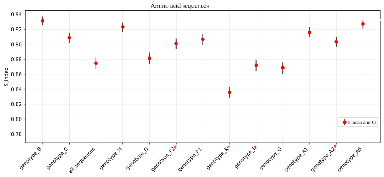
Aggregate values for amino acid sequence alignments of different HIV-1 subtypes. Red asterisks indicate subtypes represented by a limited number of sequences in the alignment.
Figure 1.
Aggregate values for amino acid sequence alignments of different HIV-1 subtypes. Red asterisks indicate subtypes represented by a limited number of sequences in the alignment.
Figure 2.
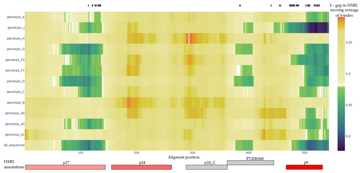
Averaged S-index panorama for the alignment of Gag amino acid sequences obtained using a sliding window of 50 amino acids. The colors correspond to the mean S-index value according to the color scale to the right of the figure. The marks above the figure indicate MSA regions corresponding to gaps in the HXB2 sequence. Below the figure, annotations of the HXB2 sequence are shown in alignment coordinates, with colors chosen randomly for contrast.
Figure 2.
Averaged S-index panorama for the alignment of Gag amino acid sequences obtained using a sliding window of 50 amino acids. The colors correspond to the mean S-index value according to the color scale to the right of the figure. The marks above the figure indicate MSA regions corresponding to gaps in the HXB2 sequence. Below the figure, annotations of the HXB2 sequence are shown in alignment coordinates, with colors chosen randomly for contrast.
Figure 3.
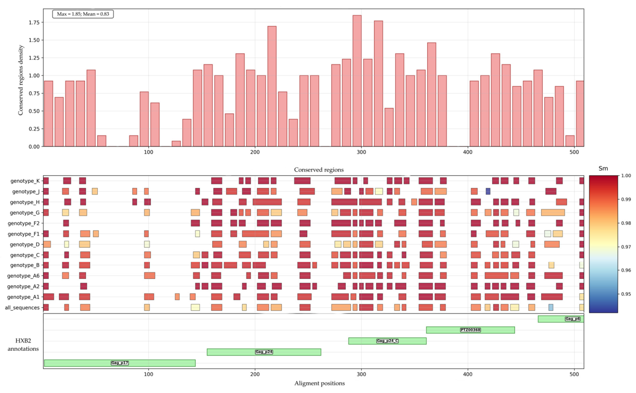
Generalized representation of conserved regions identified in Gag amino acid sequence alignments. The colors correspond to the mean S-index value according to the color scale to the right of the figure. Below the figure, annotations of the HXB2 sequence are shown in alignment coordinates.
Figure 3.
Generalized representation of conserved regions identified in Gag amino acid sequence alignments. The colors correspond to the mean S-index value according to the color scale to the right of the figure. Below the figure, annotations of the HXB2 sequence are shown in alignment coordinates.
Figure 4.
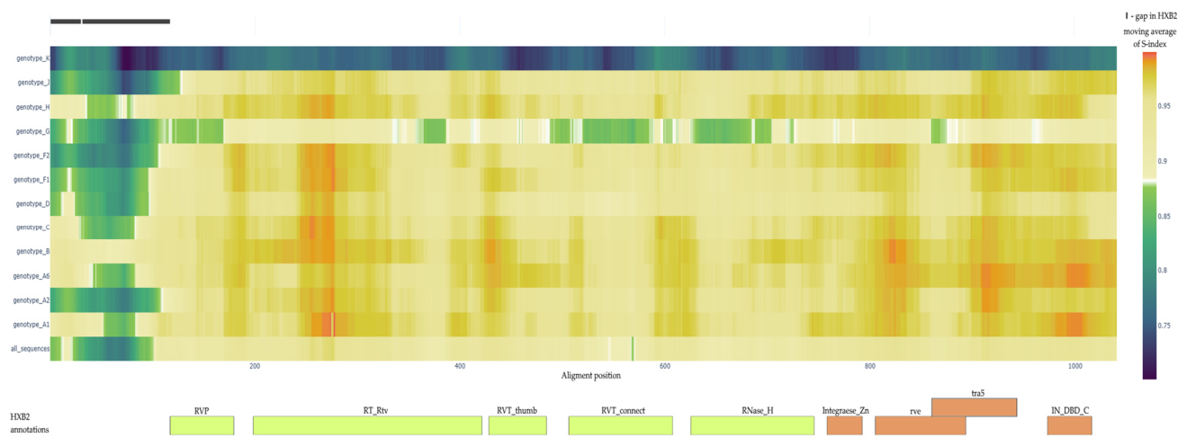
Averaged S-index panorama for the alignment of Pol amino acid sequences obtained using a sliding window of 50 amino acids. The colors correspond to the mean S-index value according to the color scale to the right of the figure. The marks above the figure indicate MSA regions corresponding to gaps in the HXB2 sequence. Below the figure, annotations of the HXB2 sequence are shown in alignment coordinates, with colors chosen randomly for contrast.
Figure 4.
Averaged S-index panorama for the alignment of Pol amino acid sequences obtained using a sliding window of 50 amino acids. The colors correspond to the mean S-index value according to the color scale to the right of the figure. The marks above the figure indicate MSA regions corresponding to gaps in the HXB2 sequence. Below the figure, annotations of the HXB2 sequence are shown in alignment coordinates, with colors chosen randomly for contrast.
Figure 5.
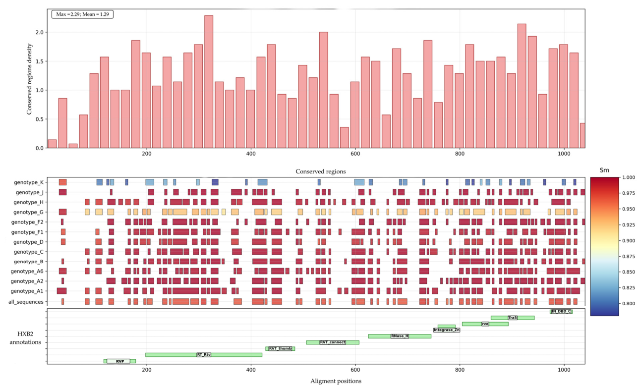
Generalized representation of conserved regions identified in Pol amino acid sequence alignments. The colors correspond to the mean S-index value according to the color scale to the right of the figure. Below the figure, annotations of the HXB2 sequence are shown in alignment coordinates.
Figure 5.
Generalized representation of conserved regions identified in Pol amino acid sequence alignments. The colors correspond to the mean S-index value according to the color scale to the right of the figure. Below the figure, annotations of the HXB2 sequence are shown in alignment coordinates.
Figure 6.
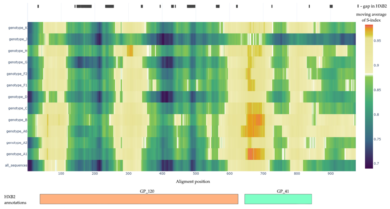
Averaged S-index panorama for the alignment of Env amino acid sequences obtained using a sliding window of 50 amino acids. The colors correspond to the mean S-index value according to the color scale to the right of the figure. The marks above the figure indicate MSA regions corresponding to gaps in the HXB2 sequence. Below the figure, annotations of the HXB2 sequence are shown in alignment coordinates, with colors chosen randomly for contrast.
Figure 6.
Averaged S-index panorama for the alignment of Env amino acid sequences obtained using a sliding window of 50 amino acids. The colors correspond to the mean S-index value according to the color scale to the right of the figure. The marks above the figure indicate MSA regions corresponding to gaps in the HXB2 sequence. Below the figure, annotations of the HXB2 sequence are shown in alignment coordinates, with colors chosen randomly for contrast.
Figure 7.
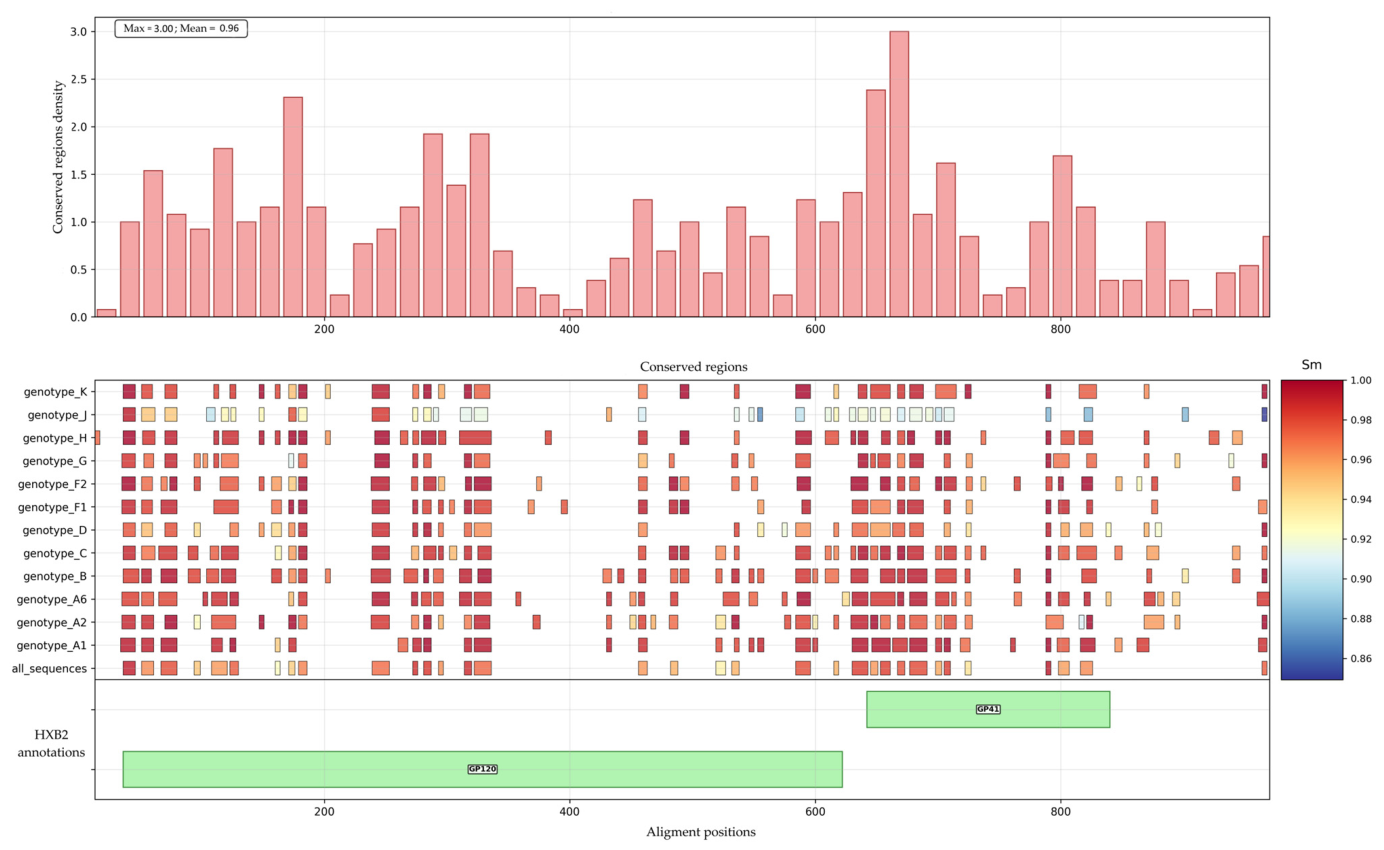
Generalized representation of conserved regions identified in Env amino acid sequence alignments. The colors correspond to the mean S-index value according to the color scale to the right of the figure. Below the figure, annotations of the HXB2 sequence are shown in alignment coordinates.
Figure 7.
Generalized representation of conserved regions identified in Env amino acid sequence alignments. The colors correspond to the mean S-index value according to the color scale to the right of the figure. Below the figure, annotations of the HXB2 sequence are shown in alignment coordinates.
Figure 8.
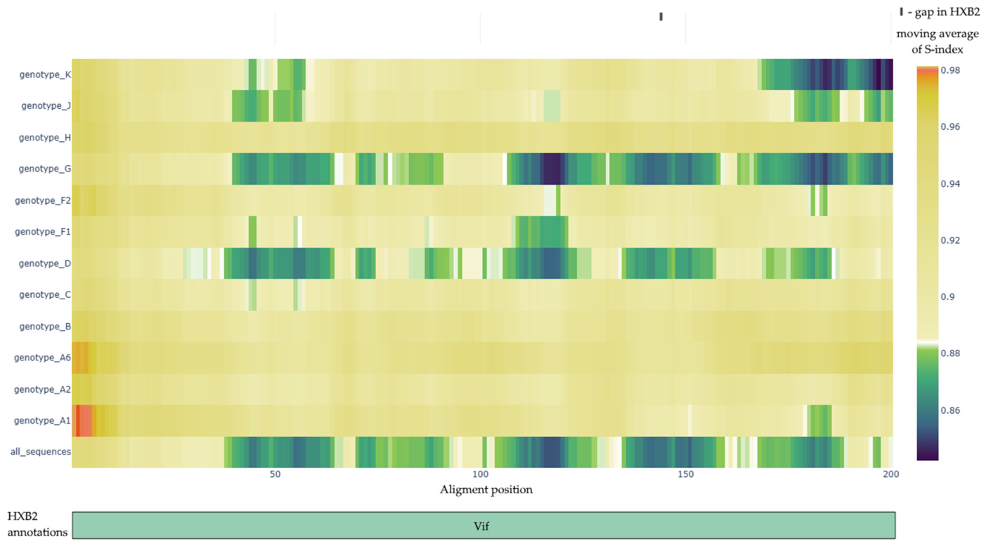
Averaged S-index panorama for the alignment of Vif amino acid sequences obtained using a sliding window of 50 amino acids. The colors correspond to the mean S-index value according to the color scale to the right of the figure. The marks above the figure indicate MSA regions corresponding to gaps in the HXB2 sequence. Below the figure, annotations of the HXB2 sequence are shown in alignment coordinates, with colors chosen randomly for contrast.
Figure 8.
Averaged S-index panorama for the alignment of Vif amino acid sequences obtained using a sliding window of 50 amino acids. The colors correspond to the mean S-index value according to the color scale to the right of the figure. The marks above the figure indicate MSA regions corresponding to gaps in the HXB2 sequence. Below the figure, annotations of the HXB2 sequence are shown in alignment coordinates, with colors chosen randomly for contrast.
Figure 9.
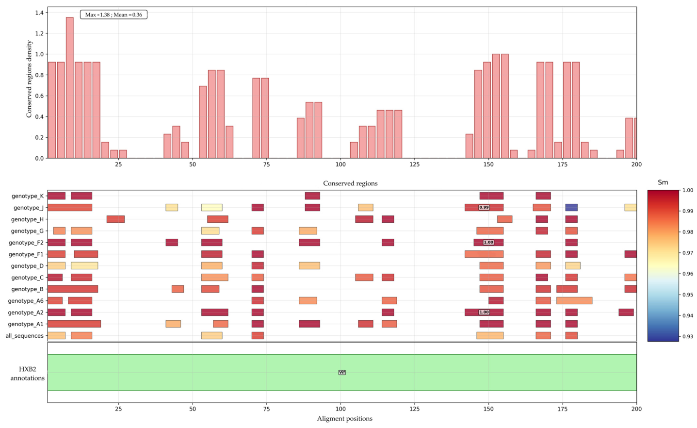
Generalized representation of conserved regions identified in Vif amino acid sequence alignments. The colors correspond to the mean S-index value according to the color scale to the right of the figure. Below the figure, annotations of the HXB2 sequence are shown in alignment coordinates.
Figure 9.
Generalized representation of conserved regions identified in Vif amino acid sequence alignments. The colors correspond to the mean S-index value according to the color scale to the right of the figure. Below the figure, annotations of the HXB2 sequence are shown in alignment coordinates.
Figure 10.
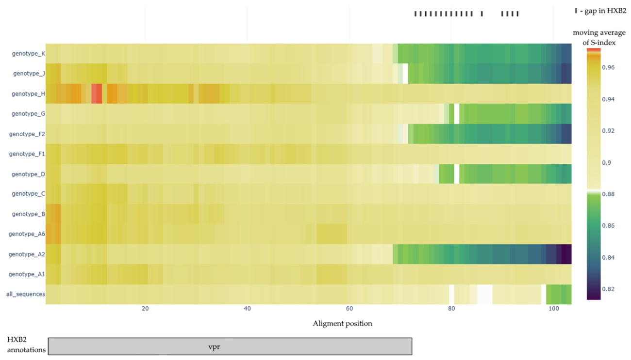
Averaged S-index panorama for the alignment of Vpr amino acid sequences obtained using a sliding window of 50 amino acids. The colors correspond to the mean S-index value according to the color scale to the right of the figure. The marks above the figure indicate MSA regions corresponding to gaps in the HXB2 sequence. Below the figure, annotations of the HXB2 sequence are shown in alignment coordinates, with colors chosen randomly for contrast.
Figure 10.
Averaged S-index panorama for the alignment of Vpr amino acid sequences obtained using a sliding window of 50 amino acids. The colors correspond to the mean S-index value according to the color scale to the right of the figure. The marks above the figure indicate MSA regions corresponding to gaps in the HXB2 sequence. Below the figure, annotations of the HXB2 sequence are shown in alignment coordinates, with colors chosen randomly for contrast.
Figure 11.
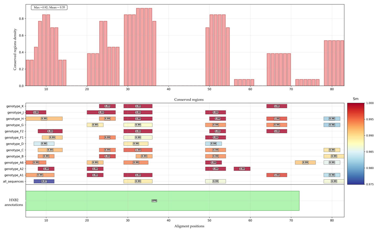
Generalized representation of conserved regions identified in Vpr amino acid sequence alignments. The colors correspond to the mean S-index value according to the color scale to the right of the figure. Below the figure, annotations of the HXB2 sequence are shown in alignment coordinates.
Figure 11.
Generalized representation of conserved regions identified in Vpr amino acid sequence alignments. The colors correspond to the mean S-index value according to the color scale to the right of the figure. Below the figure, annotations of the HXB2 sequence are shown in alignment coordinates.
Figure 12.
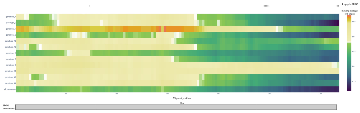
Averaged S-index panorama for the alignment of Rev amino acid sequences obtained using a sliding window of 50 amino acids. The colors correspond to the mean S-index value according to the color scale to the right of the figure. The marks above the figure indicate MSA regions corresponding to gaps in the HXB2 sequence. Below the figure, annotations of the HXB2 sequence are shown in alignment coordinates, with colors chosen randomly for contrast.
Figure 12.
Averaged S-index panorama for the alignment of Rev amino acid sequences obtained using a sliding window of 50 amino acids. The colors correspond to the mean S-index value according to the color scale to the right of the figure. The marks above the figure indicate MSA regions corresponding to gaps in the HXB2 sequence. Below the figure, annotations of the HXB2 sequence are shown in alignment coordinates, with colors chosen randomly for contrast.
Figure 13.
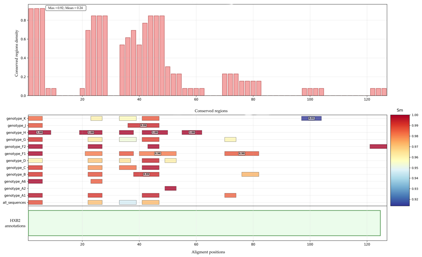
Generalized representation of conserved regions identified in Rev amino acid sequence alignments. The colors correspond to the mean S-index value according to the color scale to the right of the figure. Below the figure, annotations of the HXB2 sequence are shown in alignment coordinates.
Figure 13.
Generalized representation of conserved regions identified in Rev amino acid sequence alignments. The colors correspond to the mean S-index value according to the color scale to the right of the figure. Below the figure, annotations of the HXB2 sequence are shown in alignment coordinates.
Figure 14.
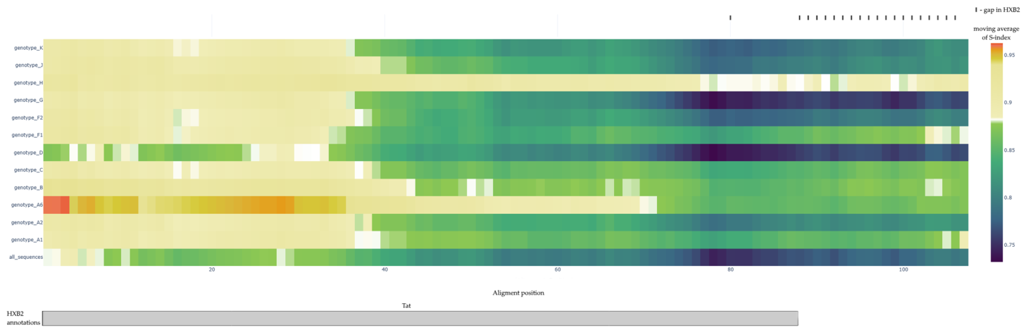
Averaged S-index panorama for the alignment of Tat amino acid sequences obtained using a sliding window of 50 amino acids. The colors correspond to the mean S-index value according to the color scale to the right of the figure. The marks above the figure indicate MSA regions corresponding to gaps in the HXB2 sequence. Below the figure, annotations of the HXB2 sequence are shown in alignment coordinates, with colors chosen randomly for contrast.
Figure 14.
Averaged S-index panorama for the alignment of Tat amino acid sequences obtained using a sliding window of 50 amino acids. The colors correspond to the mean S-index value according to the color scale to the right of the figure. The marks above the figure indicate MSA regions corresponding to gaps in the HXB2 sequence. Below the figure, annotations of the HXB2 sequence are shown in alignment coordinates, with colors chosen randomly for contrast.
Figure 15.
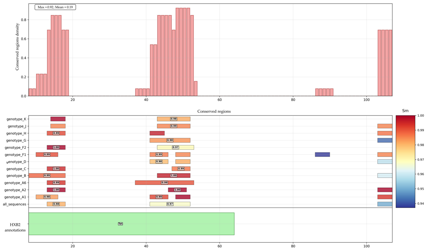
Generalized representation of conserved regions identified in Tat amino acid sequence alignments. The colors correspond to the mean S-index value according to the color scale to the right of the figure. Below the figure, annotations of the HXB2 sequence are shown in alignment coordinates.
Figure 15.
Generalized representation of conserved regions identified in Tat amino acid sequence alignments. The colors correspond to the mean S-index value according to the color scale to the right of the figure. Below the figure, annotations of the HXB2 sequence are shown in alignment coordinates.
Figure 16.
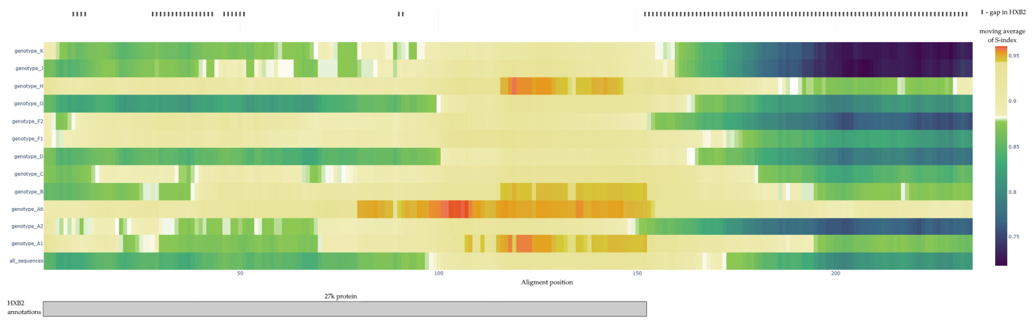
Averaged S-index panorama for the alignment of Nef amino acid sequences obtained using a sliding window of 50 amino acids. The colors correspond to the mean S-index value according to the color scale to the right of the figure. The marks above the figure indicate MSA regions corresponding to gaps in the HXB2 sequence. Below the figure, annotations of the HXB2 sequence are shown in alignment coordinates, with colors chosen randomly for contrast.
Figure 16.
Averaged S-index panorama for the alignment of Nef amino acid sequences obtained using a sliding window of 50 amino acids. The colors correspond to the mean S-index value according to the color scale to the right of the figure. The marks above the figure indicate MSA regions corresponding to gaps in the HXB2 sequence. Below the figure, annotations of the HXB2 sequence are shown in alignment coordinates, with colors chosen randomly for contrast.
Figure 17.
Generalized representation of conserved regions identified in Nef amino acid sequence alignments. The colors correspond to the mean S-index value according to the color scale to the right of the figure. Below the figure, annotations of the HXB2 sequence are shown in alignment coordinates.
Figure 17.
Generalized representation of conserved regions identified in Nef amino acid sequence alignments. The colors correspond to the mean S-index value according to the color scale to the right of the figure. Below the figure, annotations of the HXB2 sequence are shown in alignment coordinates.
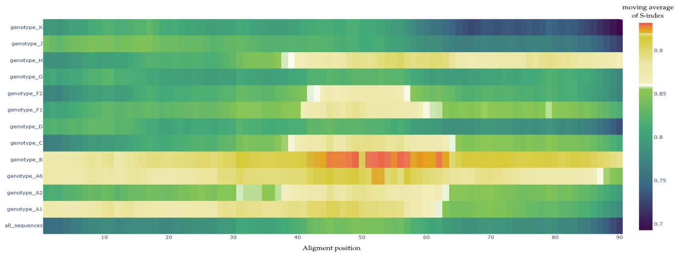
Figure 18.
Averaged S-index panorama for the alignment of Vpu amino acid sequences obtained using a sliding window of 50 amino acids. The colors correspond to the mean S-index value according to the color scale to the right of the figure. The marks above the figure indicate MSA regions corresponding to gaps in the HXB2 sequence. Below the figure, annotations of the HXB2 sequence are shown in alignment coordinates, with colors chosen randomly for contrast.
Figure 18.
Averaged S-index panorama for the alignment of Vpu amino acid sequences obtained using a sliding window of 50 amino acids. The colors correspond to the mean S-index value according to the color scale to the right of the figure. The marks above the figure indicate MSA regions corresponding to gaps in the HXB2 sequence. Below the figure, annotations of the HXB2 sequence are shown in alignment coordinates, with colors chosen randomly for contrast.
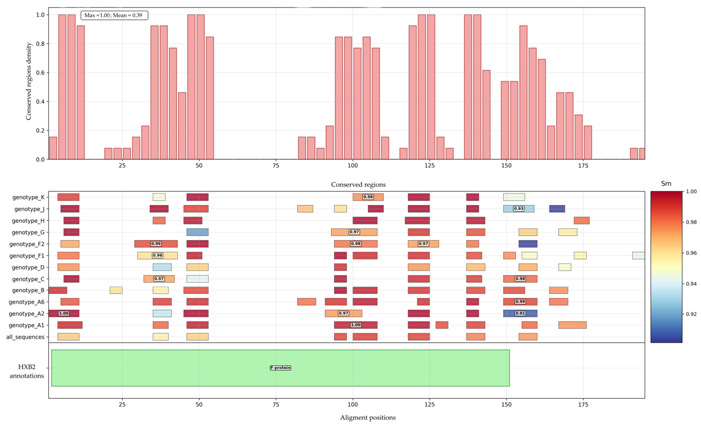
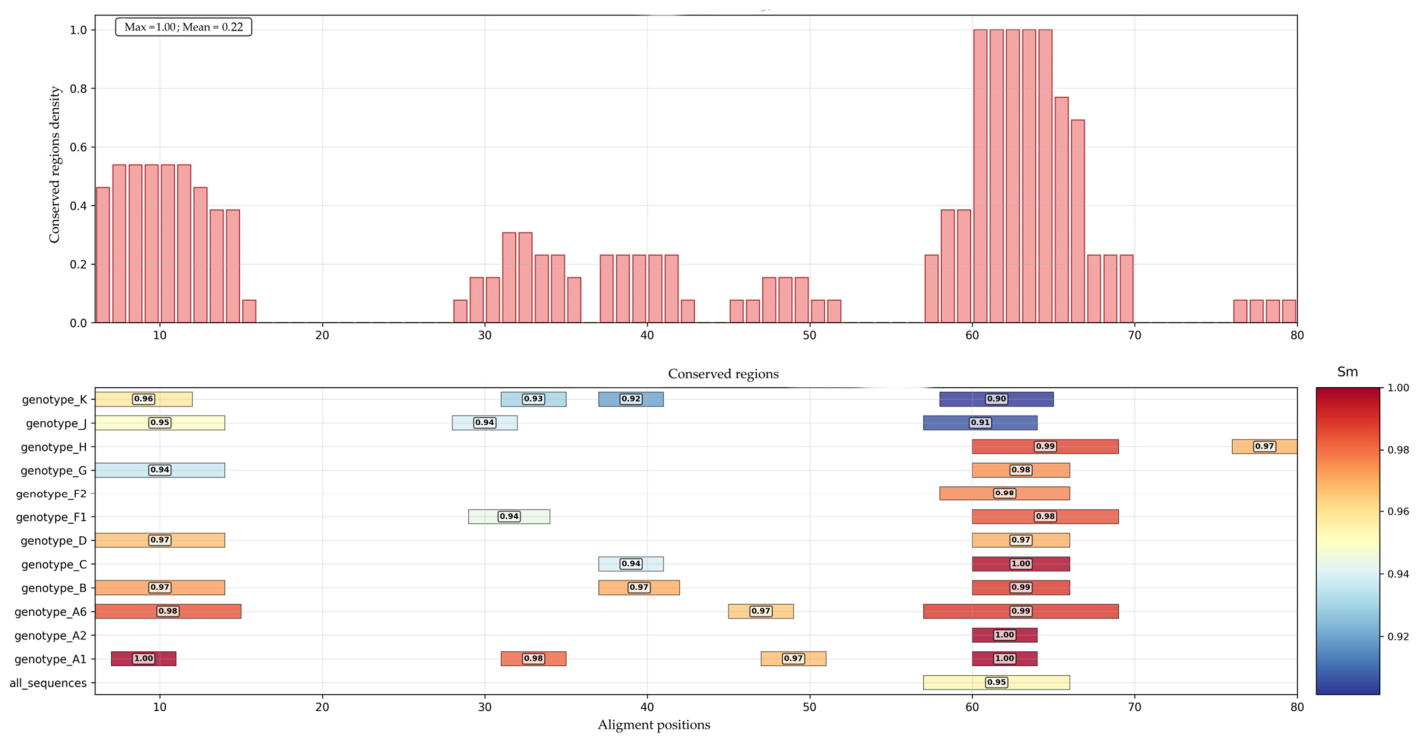
Figure 19.
Generalized representation of conserved regions identified in Vpu amino acid sequence alignments. The colors correspond to the mean S-index value according to the color scale to the right of the figure. Below the figure, annotations of the HXB2 sequence are shown in alignment coordinates.
Figure 19.
Generalized representation of conserved regions identified in Vpu amino acid sequence alignments. The colors correspond to the mean S-index value according to the color scale to the right of the figure. Below the figure, annotations of the HXB2 sequence are shown in alignment coordinates.
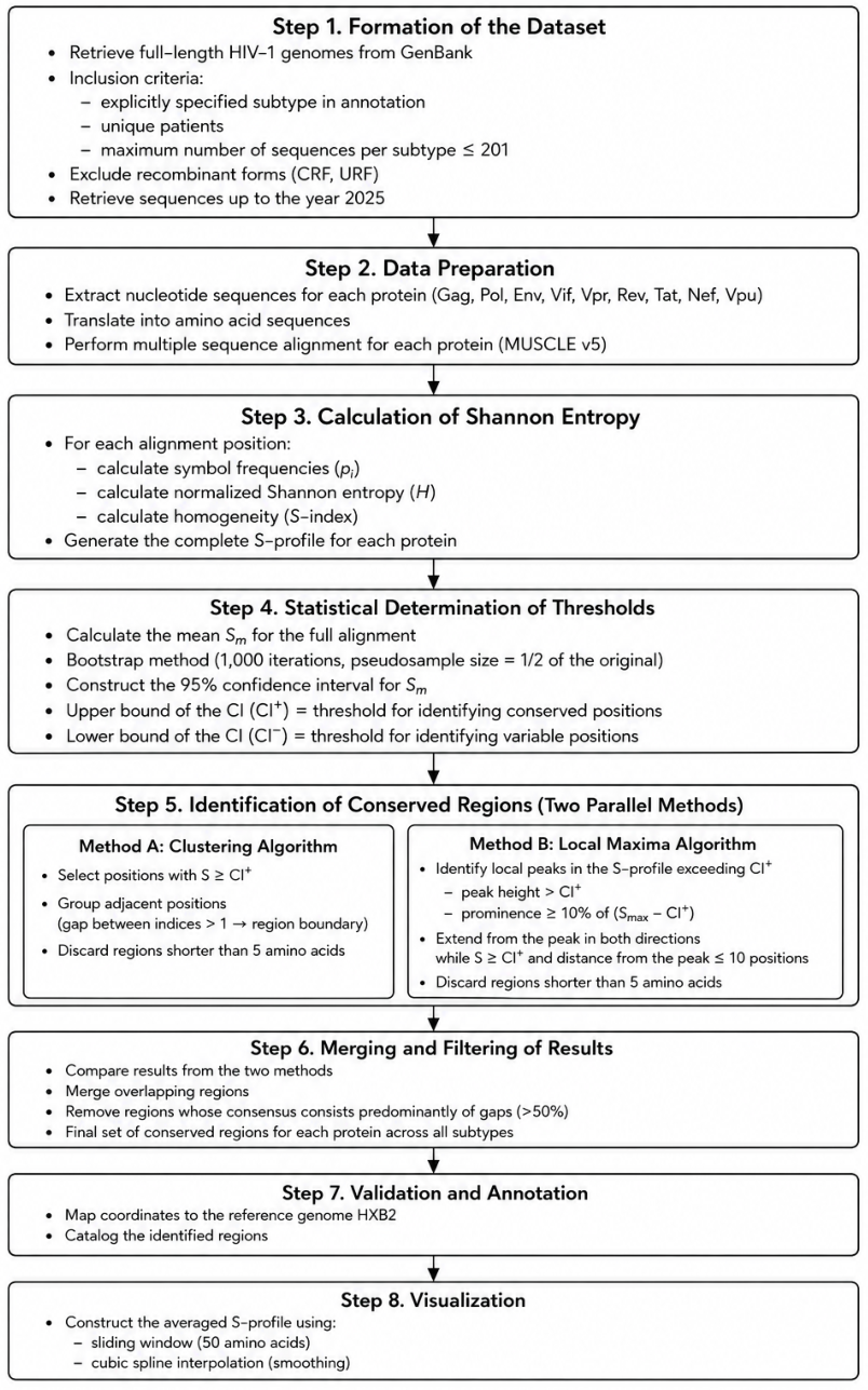
Figure 20.
Workflow of the computational pipeline used for identification of conserved regions in HIV-1 proteins.
Figure 20.
Workflow of the computational pipeline used for identification of conserved regions in HIV-1 proteins.
Table 1.
Statistical analysis of S-index values for establishing cutoff thresholds for subsequent analysis.
Table 1.
Statistical analysis of S-index values for establishing cutoff thresholds for subsequent analysis.
| Subtype | Sm | CI− | CI+ |
|---|
| All sequences | 0.8746 | 0.8671 | 0.8822 |
| A1 | 0.9158 | 0.9098 | 0.9227 |
| A2 | 0.9030 | 0.8961 | 0.9095 |
| A6 | 0.9270 | 0.9208 | 0.9327 |
| B | 0.9312 | 0.9257 | 0.9370 |
| C | 0.9086 | 0.9017 | 0.9153 |
| D | 0.8812 | 0.8733 | 0.8890 |
| F1 | 0.9063 | 0.8989 | 0.9133 |
| F2 | 0.9008 | 0.8933 | 0.9075 |
| G | 0.8685 | 0.8602 | 0.8757 |
| H | 0.9230 | 0.9163 | 0.9289 |
| J | 0.8717 | 0.8642 | 0.8792 |
| K | 0.8356 | 0.8287 | 0.8427 |
Table 2.
S-index statistics for Gag protein aligns.
Table 2.
S-index statistics for Gag protein aligns.
| Subtype | Sm | CI− | CI+ |
|---|
| All sequences | 0.9058 | 0.8896 | 0.9209 |
| A1 | 0.9393 | 0.9269 | 0.9516 |
| A2 | 0.9248 | 0.9105 | 0.9383 |
| A6 | 0.9459 | 0.9348 | 0.9560 |
| B | 0.9517 | 0.9423 | 0.9605 |
| C | 0.9242 | 0.9087 | 0.9374 |
| D | 0.9087 | 0.8937 | 0.9223 |
| F1 | 0.9216 | 0.9074 | 0.9347 |
| F2 | 0.9216 | 0.9064 | 0.9368 |
| G | 0.9143 | 0.8991 | 0.9300 |
| H | 0.9432 | 0.9309 | 0.9547 |
| J | 0.9087 | 0.8951 | 0.9228 |
| K | 0.9270 | 0.9128 | 0.9404 |
Table 3.
Statistics of conserved regions detected in Gag.
Table 3.
Statistics of conserved regions detected in Gag.
| Subtype | Conserved Regions | Mean Conserved Region Length | Sm in Conserved Regions |
|---|
| All sequences | 26 | 8.35 | 0.9856 |
| A1 | 24 | 10.67 | 0.9953 |
| A2 | 27 | 7.67 | 1.0000 |
| A6 | 24 | 9.08 | 0.9957 |
| B | 30 | 8.13 | 0.9949 |
| C | 26 | 8.12 | 0.9952 |
| D | 25 | 7.92 | 0.9863 |
| F1 | 25 | 9.24 | 0.9912 |
| F2 | 23 | 8.52 | 1.0000 |
| G | 28 | 8.71 | 0.9896 |
| H | 24 | 10.04 | 0.9982 |
| J | 25 | 8.04 | 0.9909 |
| K | 23 | 7.96 | 1.0000 |
Table 4.
Conserved region summary for Gag polyprotein aligns.
Table 4.
Conserved region summary for Gag polyprotein aligns.
| Region Name | HXB2 Coordinates | Alignment Coordinates | Length | Sm |
|---|
| Gag_CR_1 | 1–6 | 1–6 | 6 | 0.9979 |
| Gag_CR_2 | 21–25 | 21–25 | 5 | 0.9916 |
| Gag_CR_3 | 36–45 | 36–45 | 10 | 0.9871 |
| Gag_CR_4 | 96–101 | 96–101 | 6 | 0.9812 |
| Gag_CR_5 | 128–136 | 140–148 | 9 | 0.9708 |
| Gag_CR_6 | 147–157 | 159–169 | 11 | 0.9900 |
| Gag_CR_7 | 176–180 | 188–192 | 5 | 0.9777 |
| Gag_CR_8 | 190–201 | 202–213 | 12 | 0.9878 |
| Gag_CR_9 | 203–213 | 215–225 | 11 | 0.9830 |
| Gag_CR_10 | 230–240 | 242–252 | 11 | 0.9959 |
| Gag_CR_11 | 260–278 | 272–290 | 19 | 0.9841 |
| Gag_CR_12 | 280–284 | 292–296 | 5 | 0.9858 |
| Gag_CR_13 | 286–299 | 298–311 | 14 | 0.9972 |
| Gag_CR_14 | 303–308 | 315–320 | 6 | 0.9880 |
| Gag_CR_15 | 319–324 | 331–336 | 6 | 0.9843 |
| Gag_CR_16 | 326–330 | 338–342 | 5 | 0.9924 |
| Gag_CR_17 | 342–355 | 354–367 | 14 | 0.9938 |
| Gag_CR_18 | 362–367 | 374–379 | 6 | 0.9928 |
| Gag_CR_19 | 389–398 | 403–412 | 10 | 0.9876 |
| Gag_CR_20 | 402–407 | 416–421 | 6 | 0.9800 |
| Gag_CR_21 | 410–415 | 424–429 | 6 | 0.9967 |
| Gag_CR_22 | 417–424 | 431–438 | 8 | 0.9885 |
| Gag_CR_23 | 425–433 | 440–448 | 9 | 0.9741 |
| Gag_CR_24 | 440–446 | 457–463 | 7 | 0.9836 |
| Gag_CR_25 | 487–495 | 532–540 | 9 | 0.9821 |
Table 5.
S-index statistics for Pol protein aligns.
Table 5.
S-index statistics for Pol protein aligns.
| Subtype | Sm | CI− | CI+ |
|---|
| All sequences | 0.9200 | 0.9102 | 0.9286 |
| A1 | 0.9592 | 0.9523 | 0.9661 |
| A2 | 0.9463 | 0.9376 | 0.9547 |
| A6 | 0.9617 | 0.9544 | 0.9683 |
| B | 0.9654 | 0.9593 | 0.9711 |
| C | 0.9544 | 0.9466 | 0.9613 |
| D | 0.9360 | 0.9271 | 0.9444 |
| F1 | 0.9462 | 0.9377 | 0.9546 |
| F2 | 0.9444 | 0.9357 | 0.9532 |
| G | 0.8812 | 0.8732 | 0.8887 |
| H | 0.9565 | 0.9491 | 0.9635 |
| J | 0.9357 | 0.9265 | 0.9452 |
| K | 0.7588 | 0.7517 | 0.7661 |
Table 6.
Statistics of conserved regions detected in Pol.
Table 6.
Statistics of conserved regions detected in Pol.
| Subtype | Conserved Regions | Mean Conserved Region Length | Sm in Conserved Regions |
|---|
| All sequences | 50 | 9.96 | 0.9709 |
| A1 | 50 | 11.74 | 0.9971 |
| A2 | 54 | 10.15 | 1.0000 |
| A6 | 53 | 10.21 | 0.9963 |
| B | 49 | 11.14 | 0.9965 |
| C | 46 | 11.17 | 0.9965 |
| D | 47 | 9.89 | 0.9890 |
| F1 | 51 | 9.98 | 0.9945 |
| F2 | 48 | 9.85 | 1.0000 |
| G | 48 | 10.46 | 0.9278 |
| H | 50 | 10.52 | 0.9961 |
| J | 44 | 8.18 | 1.0000 |
| K | 30 | 8.60 | 0.8091 |
Table 7.
Conserved region summary for Pol polyprotein aligns.
Table 7.
Conserved region summary for Pol polyprotein aligns.
| Region Name | HXB2 Coordinates | Alignment Coordinates | Length | Sm |
|---|
| Pol_CR_1 | | 82–90 | 9 | 0.9703 |
| Pol_CR_2 | | 102–115 | 14 | 0.9696 |
| Pol_CR_3 | 11–21 | 127–137 | 11 | 0.9713 |
| Pol_CR_4 | 48–53 | 164–169 | 6 | 0.9723 |
| Pol_CR_5 | 59–67 | 175–183 | 9 | 0.9730 |
| Pol_CR_6 | 78–83 | 194–199 | 6 | 0.9728 |
| Pol_CR_7 | 85–95 | 201–211 | 11 | 0.9656 |
| Pol_CR_8 | 114–123 | 230–239 | 10 | 0.9710 |
| Pol_CR_9 | 127–131 | 243–247 | 5 | 0.9645 |
| Pol_CR_10 | 134–165 | 250–281 | 32 | 0.9684 |
| Pol_CR_11 | 168–184 | 284–300 | 17 | 0.9684 |
| Pol_CR_12 | 188–198 | 304–314 | 11 | 0.9771 |
| Pol_CR_13 | 207–221 | 323–337 | 15 | 0.9770 |
| Pol_CR_14 | 249–259 | 367–382 | 11 | 0.9666 |
| Pol_CR_15 | 279–301 | 402–424 | 23 | 0.9744 |
| Pol_CR_16 | 303–308 | 426–431 | 6 | 0.9695 |
| Pol_CR_17 | 316–335 | 440–459 | 20 | 0.9739 |
| Pol_CR_18 | 362–367 | 486–491 | 6 | 0.9729 |
| Pol_CR_19 | 369–374 | 493–498 | 6 | 0.9690 |
| Pol_CR_20 | 400–408 | 524–532 | 9 | 0.9720 |
| Pol_CR_21 | 411–419 | 535–543 | 9 | 0.9700 |
| Pol_CR_22 | 425–429 | 549–553 | 5 | 0.9640 |
| Pol_CR_23 | 469–476 | 593–600 | 8 | 0.9762 |
| Pol_CR_24 | 478–494 | 602–618 | 17 | 0.9683 |
| Pol_CR_25 | 505–509 | 629–633 | 5 | 0.9769 |
| Pol_CR_26 | 517–521 | 641–645 | 5 | 0.9679 |
| Pol_CR_27 | 536–540 | 660–664 | 5 | 0.9726 |
| Pol_CR_28 | 548–553 | 672–677 | 6 | 0.9664 |
| Pol_CR_29 | 557–575 | 681–699 | 19 | 0.9665 |
| Pol_CR_30 | 599–611 | 723–735 | 13 | 0.9776 |
| Pol_CR_31 | 613–617 | 737–741 | 5 | 0.9768 |
| Pol_CR_32 | 628–634 | 752–758 | 7 | 0.9634 |
| Pol_CR_33 | 650–654 | 774–778 | 5 | 0.9576 |
| Pol_CR_34 | 657–662 | 781–786 | 6 | 0.9697 |
| Pol_CR_35 | 675–683 | 799–807 | 9 | 0.9711 |
| Pol_CR_36 | 688–695 | 812–819 | 8 | 0.9727 |
| Pol_CR_37 | 699–707 | 823–831 | 9 | 0.9755 |
| Pol_CR_38 | 709–720 | 833–844 | 12 | 0.9675 |
| Pol_CR_39 | 738–742 | 862–866 | 5 | 0.9774 |
| Pol_CR_40 | 751–757 | 875–881 | 7 | 0.9755 |
| Pol_CR_41 | 761–779 | 885–903 | 19 | 0.9719 |
| Pol_CR_42 | 781–786 | 905–910 | 6 | 0.9681 |
| Pol_CR_43 | 792–796 | 916–920 | 5 | 0.9756 |
| Pol_CR_44 | 801–811 | 925–935 | 11 | 0.9680 |
| Pol_CR_45 | 818–824 | 942–948 | 7 | 0.9674 |
| Pol_CR_46 | 847–857 | 971–981 | 11 | 0.9708 |
| Pol_CR_47 | 859–874 | 983–998 | 16 | 0.9762 |
| Pol_CR_48 | 881–888 | 1005–1012 | 8 | 0.9766 |
| Pol_CR_49 | 894–901 | 1018–1025 | 8 | 0.9707 |
Table 8.
S-index statistics for Env protein aligns.
Table 8.
S-index statistics for Env protein aligns.
| Subtype | Sm | CI− | CI+ |
|---|
| All sequences | 0.8320 | 0.8142 | 0.8487 |
| A1 | 0.8754 | 0.8611 | 0.8900 |
| A2 | 0.8716 | 0.8564 | 0.8858 |
| A6 | 0.8886 | 0.8742 | 0.9013 |
| B | 0.9000 | 0.8872 | 0.9120 |
| C | 0.8731 | 0.8591 | 0.8867 |
| D | 0.8340 | 0.8177 | 0.8506 |
| F1 | 0.8733 | 0.8582 | 0.8878 |
| F2 | 0.8679 | 0.8529 | 0.8826 |
| G | 0.8466 | 0.8302 | 0.8619 |
| H | 0.8868 | 0.8723 | 0.9002 |
| J | 0.7989 | 0.7829 | 0.8126 |
| K | 0.8652 | 0.8497 | 0.8799 |
Table 9.
Statistics of conserved regions detected in Env.
Table 9.
Statistics of conserved regions detected in Env.
| Subtype | Conserved Regions | Mean Conserved Region Length | Sm in Conserved Regions |
|---|
| All sequences | 33 | 8.70 | 0.9666 |
| A1 | 34 | 8.94 | 0.9885 |
| A2 | 40 | 8.75 | 0.9746 |
| A6 | 40 | 9.20 | 0.9815 |
| B | 41 | 9.15 | 0.9840 |
| C | 41 | 8.68 | 0.9794 |
| D | 34 | 8.18 | 0.9642 |
| F1 | 32 | 8.88 | 0.9846 |
| F2 | 39 | 8.08 | 0.9806 |
| G | 33 | 7.97 | 0.9749 |
| H | 37 | 8.54 | 0.9881 |
| J | 36 | 7.42 | 0.9192 |
| K | 31 | 8.48 | 0.9831 |
Table 10.
Conserved region summary for Env polyprotein aligns.
Table 10.
Conserved region summary for Env polyprotein aligns.
| Region Name | HXB2 Coordinates | Alignment Coordinates | Length | Sm |
|---|
| Env_CR_1 | 34–44 | 36–46 | 11 | 0.9920 |
| Env_CR_2 | 49–59 | 51–61 | 11 | 0.9635 |
| Env_CR_3 | 65–78 | 67–80 | 14 | 0.9791 |
| Env_CR_4 | 92–97 | 94–99 | 6 | 0.9478 |
| Env_CR_5 | 106–119 | 108–121 | 14 | 0.9603 |
| Env_CR_6 | 121–128 | 123–130 | 8 | 0.9752 |
| Env_CR_7 | 202–206 | 272–276 | 5 | 0.9872 |
| Env_CR_8 | 211–217 | 281–287 | 7 | 0.9846 |
| Env_CR_9 | 223–227 | 293–297 | 5 | 0.9624 |
| Env_CR_10 | 244–250 | 314–320 | 7 | 0.9882 |
| Env_CR_11 | 252–266 | 322–336 | 15 | 0.9718 |
| Env_CR_12 | 377–384 | 456–463 | 8 | 0.9603 |
| Env_CR_13 | 417–425 | 519–527 | 9 | 0.9303 |
| Env_CR_14 | 430–436 | 532–538 | 7 | 0.9540 |
| Env_CR_15 | 474–486 | 584–596 | 13 | 0.9790 |
| Env_CR_16 | 505–509 | 615–619 | 5 | 0.9542 |
| Env_CR_17 | 518–531 | 630–643 | 14 | 0.9834 |
| Env_CR_18 | 533–539 | 645–651 | 7 | 0.9601 |
| Env_CR_19 | 541–549 | 653–661 | 9 | 0.9828 |
| Env_CR_20 | 555–561 | 667–673 | 7 | 0.9774 |
| Env_CR_21 | 565–579 | 677–691 | 15 | 0.9796 |
| Env_CR_22 | 586–591 | 698–703 | 6 | 0.9559 |
| Env_CR_23 | 593–598 | 705–710 | 6 | 0.9829 |
| Env_CR_24 | 610–614 | 722–727 | 6 | 0.9378 |
| Env_CR_25 | 675–679 | 788–792 | 5 | 0.9937 |
| Env_CR_26 | 685–694 | 798–807 | 10 | 0.9584 |
| Env_CR_27 | 703–713 | 816–826 | 11 | 0.9630 |
| Env_CR_28 | 843–847 | 964–968 | 5 | 0.9748 |
Table 11.
S-index statistics for Vif protein aligns.
Table 11.
S-index statistics for Vif protein aligns.
| Subtype | Sm | CI− | CI+ |
|---|
| All sequences | 0.8809 | 0.8538 | 0.9075 |
| A1 | 0.9183 | 0.8950 | 0.9372 |
| A2 | 0.9132 | 0.8869 | 0.9366 |
| A6 | 0.9322 | 0.9137 | 0.9497 |
| B | 0.9221 | 0.9013 | 0.9434 |
| C | 0.9081 | 0.8833 | 0.9299 |
| D | 0.8838 | 0.8577 | 0.9101 |
| F1 | 0.8999 | 0.8760 | 0.9254 |
| F2 | 0.9084 | 0.8808 | 0.9317 |
| G | 0.8795 | 0.8529 | 0.9070 |
| H | 0.9314 | 0.9119 | 0.9503 |
| J | 0.9010 | 0.8735 | 0.9251 |
| K | 0.8982 | 0.8700 | 0.9239 |
Table 12.
Statistics of conserved regions detected in Vif.
Table 12.
Statistics of conserved regions detected in Vif.
| Subtype | Conserved Regions | Mean Conserved Region Length | Sm in Conserved Regions |
|---|
| All sequences | 7 | 7.00 | 0.9832 |
| A1 | 10 | 7.40 | 0.9941 |
| A2 | 9 | 7.22 | 1.0000 |
| A6 | 8 | 7.13 | 0.9900 |
| B | 8 | 7.88 | 0.9930 |
| C | 10 | 6.40 | 0.9913 |
| D | 8 | 7.25 | 0.9794 |
| F1 | 8 | 7.38 | 0.9955 |
| F2 | 8 | 7.00 | 1.0000 |
| G | 8 | 6.38 | 0.9854 |
| H | 7 | 5.86 | 0.9958 |
| J | 10 | 7.60 | 0.9785 |
| K | 5 | 7.00 | 1.0000 |
Table 13.
Conserved region summary for Vif polyprotein aligns.
Table 13.
Conserved region summary for Vif polyprotein aligns.
| Region Name | HXB2 Coordinates | Alignment Coordinates | Length | Sm |
|---|
| VIf_CR_1 | 1–16 | 1–16 | 16 | 0.9761 |
| VIf_CR_2 | 52–59 | 53–60 | 8 | 0.9738 |
| VIf_CR_3 | 68–72 | 70–74 | 5 | 0.9923 |
| VIf_CR_4 | 141–150 | 146–155 | 10 | 0.9777 |
| VIf_CR_5 | 161–166 | 166–171 | 6 | 0.9877 |
| VIf_CR_6 | 171–175 | 176–180 | 5 | 0.9906 |
Table 14.
S-index statistics for Vpr protein aligns.
Table 14.
S-index statistics for Vpr protein aligns.
| Subtype | Sm | CI− | CI+ |
|---|
| All sequences | 0.9091 | 0.8680 | 0.9441 |
| A1 | 0.9378 | 0.9068 | 0.9649 |
| A2 | 0.9026 | 0.8602 | 0.9398 |
| A6 | 0.9434 | 0.9134 | 0.9697 |
| B | 0.9400 | 0.9079 | 0.9663 |
| C | 0.9290 | 0.8976 | 0.9554 |
| D | 0.9093 | 0.8655 | 0.9447 |
| F1 | 0.9336 | 0.9058 | 0.9589 |
| F2 | 0.9070 | 0.8697 | 0.9429 |
| G | 0.9063 | 0.8649 | 0.9403 |
| H | 0.9442 | 0.9166 | 0.9666 |
| J | 0.9100 | 0.8742 | 0.9442 |
| K | 0.9024 | 0.8641 | 0.9392 |
Table 15.
Statistics of conserved regions detected in Vpr.
Table 15.
Statistics of conserved regions detected in Vpr.
| Subtype | Conserved Regions | Mean Conserved Region Length | Sm in Conserved Regions |
|---|
| All sequences | 4 | 6.50 | 0.9843 |
| A1 | 5 | 6.40 | 0.9946 |
| A2 | 4 | 5.25 | 1.0000 |
| A6 | 6 | 5.66 | 0.9929 |
| B | 5 | 5.40 | 0.9937 |
| C | 5 | 6.20 | 0.9935 |
| D | 3 | 6.00 | 0.9854 |
| F1 | 4 | 6.25 | 0.9932 |
| F2 | 4 | 6.50 | 1.0000 |
| G | 5 | 6.00 | 0.9892 |
| H | 6 | 6.50 | 0.9940 |
| J | 4 | 7.00 | 1.0000 |
| K | 3 | 6.33 | 1.0000 |
Table 16.
Conserved region summary for Vpr polyprotein aligns.
Table 16.
Conserved region summary for Vpr polyprotein aligns.
| Region Name | HXB2 Coordinates | Alignment Coordinates | Length | Sm |
|---|
| Vpr_CR_1 | 7–12 | 7–12 | 6 | 0.9749 |
| Vpr_CR_2 | 29–36 | 29–36 | 8 | 0.9891 |
| Vpr_CR_3 | 49–54 | 49–54 | 6 | 0.9864 |
| Vpr_CR_4 | | 78–83 | 6 | 0.9867 |
Table 17.
S-index statistics for Rev protein aligns.
Table 17.
S-index statistics for Rev protein aligns.
| Subtype | Sm | CI− | CI+ |
|---|
| All sequences | 0.8246 | 0.7866 | 0.8613 |
| A1 | 0.8713 | 0.8358 | 0.9057 |
| A2 | 0.8622 | 0.8260 | 0.8968 |
| A6 | 0.9064 | 0.8826 | 0.9306 |
| B | 0.9047 | 0.8750 | 0.9320 |
| C | 0.8562 | 0.8187 | 0.8868 |
| D | 0.8365 | 0.8018 | 0.8696 |
| F1 | 0.8751 | 0.8384 | 0.9079 |
| F2 | 0.8772 | 0.8421 | 0.9111 |
| G | 0.8408 | 0.8026 | 0.8778 |
| H | 0.9295 | 0.9092 | 0.9493 |
| J | 0.8524 | 0.8161 | 0.8871 |
| K | 0.8610 | 0.8287 | 0.8932 |
Table 18.
Statistics of conserved regions detected in Rev.
Table 18.
Statistics of conserved regions detected in Rev.
| Subtype | Conserved Regions | Mean Conserved Region Length | Sm in Conserved Regions |
|---|
| All sequences | 4 | 6.50 | 0.9694 |
| A1 | 4 | 6.00 | 0.9919 |
| A2 | 1 | 5.00 | 1.0000 |
| A6 | 2 | 5.50 | 0.9928 |
| B | 4 | 7.25 | 0.9864 |
| C | 4 | 6.50 | 0.9877 |
| D | 5 | 5.80 | 0.9702 |
| F1 | 5 | 9.20 | 0.9872 |
| F2 | 4 | 6.00 | 1.0000 |
| G | 5 | 6.20 | 0.9715 |
| H | 5 | 8.40 | 1.0000 |
| J | 2 | 9.00 | 0.9905 |
| K | 5 | 6.60 | 0.9603 |
Table 19.
Conserved region summary for Rev polyprotein aligns.
Table 19.
Conserved region summary for Rev polyprotein aligns.
| Region Name | HXB2 Coordinates | Alignment Coordinates | Length | Sm |
|---|
| Rev_CR_1 | 1–6 | 1–6 | 6 | 0.9877 |
| Rev_CR_2 | 22–27 | 22–27 | 6 | 0.9711 |
| Rev_CR_3 | 33–39 | 33–39 | 7 | 0.9466 |
| Rev_CR_4 | 41–47 | 41–47 | 7 | 0.9721 |
Table 20.
S-index statistics for Tat protein aligns.
Table 20.
S-index statistics for Tat protein aligns.
| Subtype | Sm | CI− | CI+ |
|---|
| All sequences | 0.8205 | 0.7731 | 0.8662 |
| A1 | 0.8752 | 0.8389 | 0.9083 |
| A2 | 0.8532 | 0.8128 | 0.8922 |
| A6 | 0.9045 | 0.8728 | 0.9330 |
| B | 0.8912 | 0.8560 | 0.9208 |
| C | 0.8726 | 0.8358 | 0.9102 |
| D | 0.8179 | 0.7730 | 0.8641 |
| F1 | 0.8675 | 0.8273 | 0.9058 |
| F2 | 0.8414 | 0.7996 | 0.8810 |
| G | 0.8285 | 0.7876 | 0.8695 |
| H | 0.9045 | 0.8724 | 0.9327 |
| J | 0.8539 | 0.8068 | 0.8912 |
| K | 0.8413 | 0.8002 | 0.8797 |
Table 21.
Statistics of conserved regions detected in Tat.
Table 21.
Statistics of conserved regions detected in Tat.
| Subtype | Conserved Regions | Mean Conserved Region Length | Sm in Conserved Regions |
|---|
| All sequences | 3 | 7.66 | 0.9659 |
| A1 | 4 | 5.75 | 0.9922 |
| A2 | 3 | 5.66 | 1.0000 |
| A6 | 2 | 11.50 | 0.9923 |
| B | 3 | 8.66 | 0.9821 |
| C | 2 | 6.00 | 0.9910 |
| D | 3 | 5.33 | 0.9729 |
| F1 | 5 | 5.60 | 0.9770 |
| F2 | 2 | 8.50 | 0.9849 |
| G | 2 | 8.50 | 0.9631 |
| H | 3 | 5.33 | 0.9917 |
| J | 3 | 6.66 | 0.9855 |
| K | 2 | 7.50 | 0.9907 |
Table 22.
Conserved region summary for Tat polyprotein aligns.
Table 22.
Conserved region summary for Tat polyprotein aligns.
| Region Name | HXB2 Coordinates | Alignment Coordinates | Length | Sm |
|---|
| Tat_CR_1 | 13–18 | 13–18 | 6 | 0.9807 |
| Tat_CR_2 | 41–52 | 41–52 | 12 | 0.9676 |
Table 23.
S-index statistics for Nef protein aligns.
Table 23.
S-index statistics for Nef protein aligns.
| Subtype | Sm | CI− | CI+ |
|---|
| All sequences | 0.8662 | 0.8381 | 0.8936 |
| A1 | 0.9016 | 0.8773 | 0.9254 |
| A2 | 0.8601 | 0.8365 | 0.8837 |
| A6 | 0.9263 | 0.9058 | 0.9442 |
| B | 0.9047 | 0.8825 | 0.9274 |
| C | 0.8920 | 0.8694 | 0.9156 |
| D | 0.8562 | 0.8292 | 0.8826 |
| F1 | 0.8911 | 0.8688 | 0.9127 |
| F2 | 0.8689 | 0.8436 | 0.8926 |
| G | 0.8548 | 0.8267 | 0.8806 |
| H | 0.9117 | 0.8890 | 0.9317 |
| J | 0.8511 | 0.8228 | 0.8766 |
| K | 0.8474 | 0.8219 | 0.8716 |
Table 24.
Statistics of conserved regions detected in Nef.
Table 24.
Statistics of conserved regions detected in Nef.
| Subtype | Conserved Regions | Mean Conserved Region Length | Sm in Conserved Regions |
|---|
| All sequences | 8 | 7.25 | 0.9755 |
| A1 | 9 | 8.22 | 0.9889 |
| A2 | 7 | 9.28 | 0.9736 |
| A6 | 10 | 7.50 | 0.9895 |
| B | 10 | 7.10 | 0.9836 |
| C | 7 | 8.00 | 0.9823 |
| D | 8 | 6.88 | 0.9657 |
| F1 | 11 | 7.00 | 0.9754 |
| F2 | 7 | 9.71 | 0.9705 |
| G | 7 | 8.42 | 0.9700 |
| H | 7 | 7.00 | 0.9940 |
| J | 10 | 7.00 | 0.9747 |
| K | 7 | 7.57 | 0.9797 |
Table 25.
Conserved region summary for Nef polyprotein aligns.
Table 25.
Conserved region summary for Nef polyprotein aligns.
| Region Name | HXB2 Coordinates | Alignment Coordinates | Length | Sm |
|---|
| Nef_CR_1 | 1–7 | 1–7 | 8 | 0.9654 |
| Nef_CR_2 | 66–70 | 94–98 | 5 | 0.9885 |
| Nef_CR_3 | 72–80 | 100–108 | 9 | 0.9893 |
| Nef_CR_4 | 90–97 | 118–125 | 8 | 0.9887 |
| Nef_CR_5 | 109–115 | 137–143 | 7 | 0.9784 |
| Nef_CR_6 | | 154–160 | 7 | 0.9745 |
Table 26.
S-index statistics for Vpu protein aligns.
Table 26.
S-index statistics for Vpu protein aligns.
| Genotype | Sm | CI− | CI+ |
|---|
| All sequences | 0.7839 | 0.7307 | 0.8321 |
| A1 | 0.8602 | 0.8155 | 0.9004 |
| A2 | 0.8446 | 0.8025 | 0.8844 |
| A6 | 0.8861 | 0.8448 | 0.9221 |
| B | 0.9046 | 0.8722 | 0.9346 |
| C | 0.8327 | 0.7889 | 0.8733 |
| D | 0.7975 | 0.7504 | 0.8457 |
| F1 | 0.8412 | 0.7982 | 0.8820 |
| F2 | 0.8167 | 0.7654 | 0.8665 |
| G | 0.8029 | 0.7593 | 0.8437 |
| H | 0.8479 | 0.8069 | 0.8862 |
| J | 0.8025 | 0.7604 | 0.8412 |
| K | 0.7725 | 0.7232 | 0.8194 |
Table 27.
Statistics of conserved regions detected in Vpu.
Table 27.
Statistics of conserved regions detected in Vpu.
| Genotype | Conserved Regions | Mean Conserved Region Length | Sm in Conserved Regions |
|---|
| All sequences | 1 | 10.00 | 0.9541 |
| A1 | 4 | 5.00 | 0.9873 |
| A2 | 1 | 5.00 | 1.0000 |
| A6 | 3 | 9.33 | 0.9799 |
| B | 3 | 7.33 | 0.9778 |
| C | 2 | 6.00 | 0.9687 |
| D | 2 | 8.00 | 0.9687 |
| F1 | 2 | 8.00 | 0.9642 |
| F2 | 1 | 9.00 | 0.9766 |
| G | 2 | 8.00 | 0.9553 |
| H | 2 | 7.50 | 0.9783 |
| J | 3 | 7.33 | 0.9315 |
| K | 4 | 6.25 | 0.9270 |
Table 28.
Number of analyzed sequences by region, protein, and genotype.
Table 28.
Number of analyzed sequences by region, protein, and genotype.
| Subtype | Env | Gag | Nef | Pol | Rev | Tat | Vpu |
|---|
| A1 | 111 | 105 | 106 | 106 | 105 | 105 | 106 |
| A2 | 8 | 9 | 8 | 9 | 9 | 9 | 8 |
| A6 | 193 | 196 | 196 | 194 | 194 | 195 | 195 |
| B | 199 | 200 | 199 | 196 | 197 | 200 | 200 |
| C | 190 | 197 | 196 | 189 | 191 | 201 | 200 |
| D | 93 | 98 | 97 | 99 | 95 | 93 | 95 |
| F1 | 61 | 62 | 61 | 56 | 55 | 60 | 61 |
| F2 | 11 | 13 | 10 | 12 | 9 | 13 | 10 |
| G | 89 | 91 | 93 | 96 | 96 | 96 | 92 |
| H | 100 | 98 | 97 | 99 | 10 | 98 | 96 |
| J | 16 | 22 | 10 | 16 | 16 | 16 | 16 |
| K | 12 | 12 | 12 | 16 | 11 | 11 | 11 |
| All subtypes | 1083 | 1103 | 1085 | 1088 | 988 | 1097 | 1090 |



 ,
,