
Residue Folding Degree—Relationship to Secondary Structure Categories and Use as Collective Variable


Abstract
:1. Introduction
2. Results and Discussions
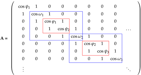
2.1. Calculation of the Residue Folding Degree
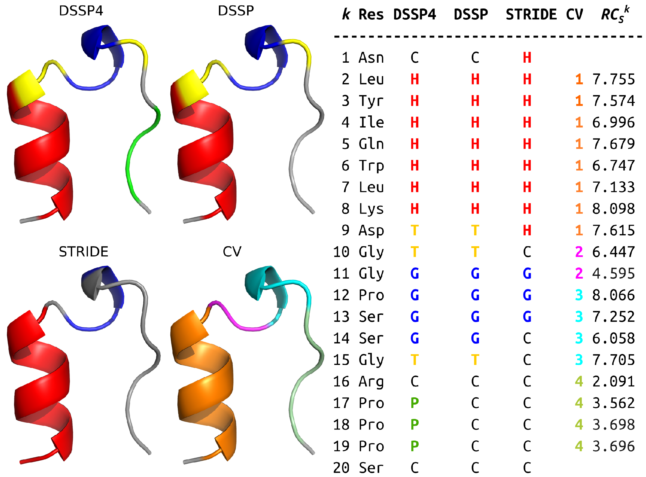
2.2. and SS Categories
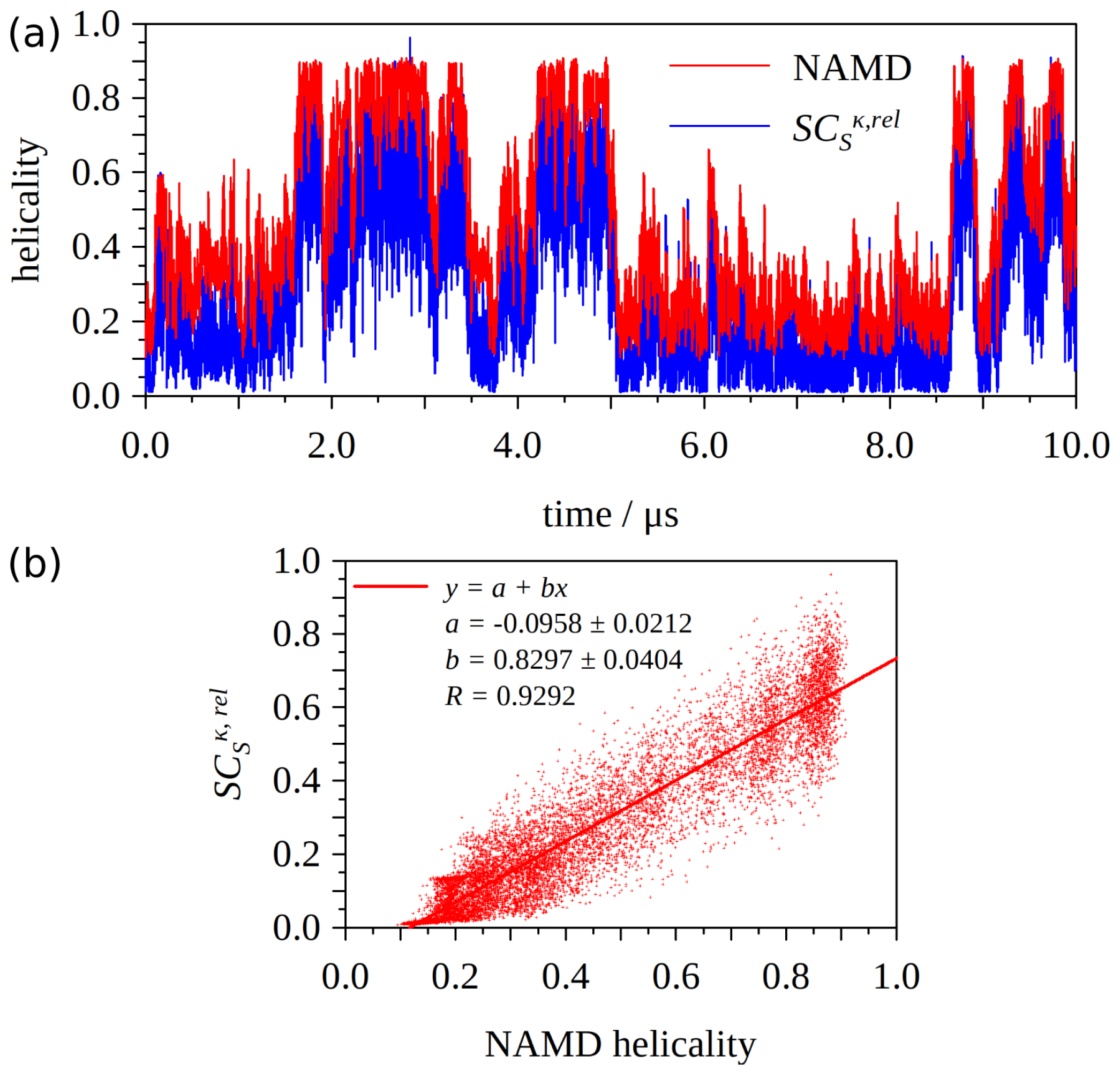
2.3. and Helical Content
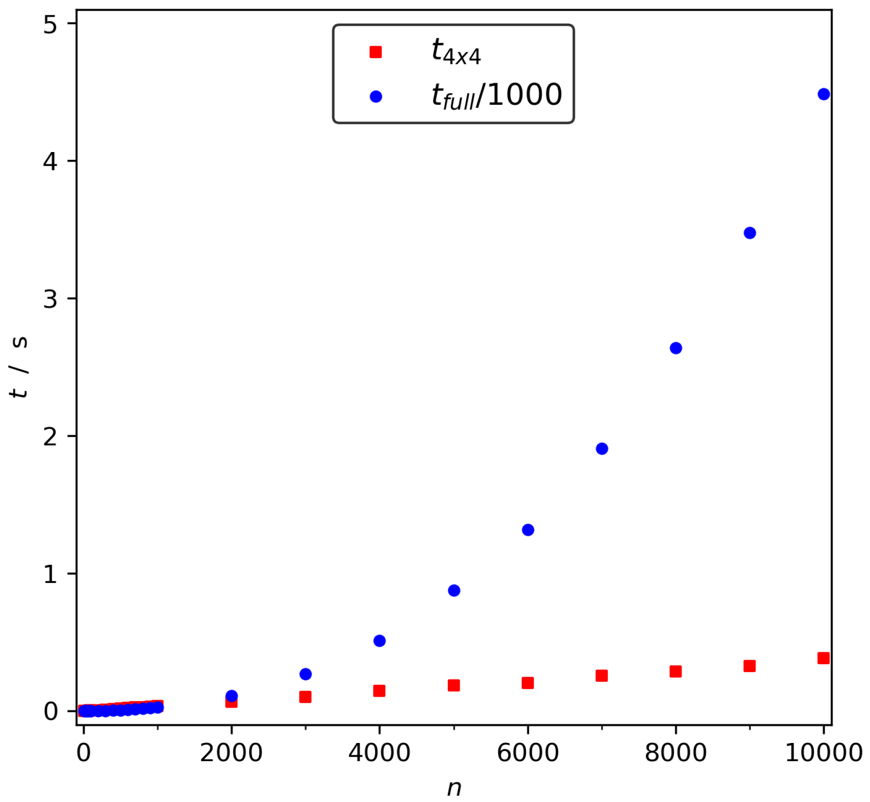
2.4. as a General Collective Variable
3. Materials and Methods
3.1. Selection of the Protein Structure Database
3.2. Molecular Dynamics
Supplementary Materials
Author Contributions
Funding
Institutional Review Board Statement
Informed Consent Statement
Data Availability Statement
Conflicts of Interest
References
- Senior, A.W.; Evans, R.; Jumper, J.; Kirkpatrick, J.; Sifre, L.; Green, T.; Qin, C.; Žídek, A.; Nelson, A.W.R.; Bridgland, A.; et al. Improved protein structure prediction using potentials from deep learning. Nature 2020, 577, 706–710. [Google Scholar] [CrossRef] [PubMed]
- Lane, T.J.; Shukla, D.; Beauchamp, K.A.; Pande, V.S. To milliseconds and beyond: Challenges in the simulation of protein folding. Curr. Opin. Struct. Biol. 2013, 23, 58–65. [Google Scholar] [CrossRef] [Green Version]
- Finkelstein, A.V.; Badretdin, A.J.; Galzitskaya, O.V.; Ivankov, D.N.; Bogatyreva, N.S.; Garbuzynskiy, S.O. There and back again: Two views on the protein folding puzzle. Phys. Life Rev. 2017, 21, 56–71. [Google Scholar] [CrossRef] [PubMed]
- Bowman, G.R.; Vijay, P.S.; Noé, F. An Introduction to Markov State Models and Their Application to Long Timescale Molecular Simulation; Springer: Heidelberg, Germany, 2014. [Google Scholar] [CrossRef]
- Kumar, S.; Rosenberg, J.M.; Bouzida, D.; Swendsen, R.H.; Kollman, P.A. The weighted histogram analysis method for free-energy calculations on biomolecules. I. The method. J. Comput. Chem. 1992, 13, 1011–1021. [Google Scholar] [CrossRef]
- Harada, R.; Sladek, V.; Shigeta, Y. Nontargeted Parallel Cascade Selection Molecular Dynamics Using Time-Localized Prediction of Conformational Transitions in Protein Dynamics. J. Chem. Theory Comput. 2019, 15, 5144–5153. [Google Scholar] [CrossRef] [PubMed]
- Phillips, J.C.; Braun, R.; Wang, W.; Gumbart, J.; Tajkhorshid, E.; Villa, E.; Chipot, C.; Skeel, R.D.; Kale, L.; Schulten, K. Scalable molecular dynamics with NAMD. J. Comput. Chem. 2005, 26, 1781–1802. [Google Scholar] [CrossRef] [Green Version]
- Pietrucci, F.; Laio, A. A Collective Variable for the Efficient Exploration of Protein Beta-Sheet Structures: Application to SH3 and GB1. J. Chem. Theory Comput. 2009, 5, 2197–2201. [Google Scholar] [CrossRef] [PubMed]
- Sladek, V.; Harada, R.; Shigeta, Y. Protein Dynamics and the Folding Degree. J. Chem. Inf. Model. 2020, 60, 1559–1567. [Google Scholar] [CrossRef] [PubMed]
- Estrada, E. Characterization of 3D molecular structure. Chem. Phys. Lett. 2000, 319, 713–718. [Google Scholar] [CrossRef]
- De la Peña, J.A.; Gutman, I.; Rada, J. Estimating the Estrada index. Linear Algebra Appl. 2007, 427, 70–76. [Google Scholar] [CrossRef] [Green Version]
- Estrada, E. Characterization of the folding degree of proteins. Bioinformatics 2002, 18, 697–704. [Google Scholar] [CrossRef]
- Estrada, E. Characterization of the amino acid contribution to the folding degree of proteins. Proteins 2004, 54, 727–737. [Google Scholar] [CrossRef]
- Estrada, E. The Many Facets of the Estrada Indices of Graphs and Networks; Springer Nature: Cham, Switzerland, 2021. [Google Scholar] [CrossRef]
- Estrada, E.; Rodríguez-Velázquez, J.A. Subgraph centrality in complex networks. Phys. Rev. E 2005, 71, 056103. [Google Scholar] [CrossRef] [Green Version]
- Hamelryck, T.; Manderick, B. PDB file parser and structure class implemented in Python. Bioinformatics 2003, 19, 2308–2310. [Google Scholar] [CrossRef] [PubMed] [Green Version]
- Frishman, D.; Argos, P. Knowledge-Based Protein Secondary Structure Assignment. Proteins 1995, 23, 566–579. [Google Scholar] [CrossRef] [PubMed]
- Zacharias, J.; Knapp, E.W. Protein Secondary Structure Classification Revisited: Processing DSSP Information with PSSC. J. Chem. Inf. Model. 2014, 54, 2166–2179. [Google Scholar] [CrossRef] [PubMed]
- Martin, J.; Letellier, G.; Marin, A.; Taly, J.F.; de Brevern, A.G.; Gibrat, J.F. Protein secondary structure assignment revisited: A detailed analysis of different assignment methods. BMC Struct. Biol. 2005, 5, 17. [Google Scholar] [CrossRef] [Green Version]
- Chebrek, R.; Leonard, S.; de Brevern, A.G.; Gelly, J.C. PolyprOnline: Polyproline helix II and secondary structure assignment database. Database 2014, 2014, bau102. [Google Scholar] [CrossRef] [Green Version]
- Neidigh, J.W.; Fesinmeyer, R.M.; Andersen, N.H. Designing a 20-residue protein. Nat. Struct. Biol. 2002, 9, 425–430. [Google Scholar] [CrossRef]
- Sladek, V.; Yamamoto, Y.; Harada, R.; Shoji, M.; Shigeta, Y.; Sladek, V. pyProGA-A PyMOL plugin for protein residue network analysis. PLoS ONE 2021, 16, e0255167. [Google Scholar] [CrossRef] [PubMed]
- Marcos-Alcalde, I.; Setoain, J.; Mendieta-Moreno, J.I.; Mendieta, J.; Gómez-Puertas, P. MEPSA: Minimum energy pathway analysis for energy landscapes. Bioinformatics 2015, 31, 3853–3855. [Google Scholar] [CrossRef] [Green Version]
- Marcos-Alcalde, I.; López-Viñas, E.; Gómez-Puertas, P. MEPSAnd: Minimum energy path surface analysis over n-dimensional surfaces. Bioinformatics 2019, 36, 956–958. [Google Scholar] [CrossRef]
- Streicher, W.W.; Makhatadze, G.I. Unfolding Thermodynamics of Trp-Cage, a 20 Residue Miniprotein, Studied by Differential Scanning Calorimetry and Circular Dichroism Spectroscopy. Biochemistry 2007, 46, 2876–2880. [Google Scholar] [CrossRef] [PubMed]
- Barua, B.; Lin, J.C.; Williams, V.D.; Kummler, P.; Neidigh, J.W.; Andersen, N.H. The Trp-cage: Optimizing the stability of a globular miniprotein. Protein Eng. Des. Sel. 2008, 21, 171–185. [Google Scholar] [CrossRef] [Green Version]
- Zhou, R. Trp-cage: Folding free energy landscape in explicit water. Proc. Natl. Acad. Sci. USA 2003, 100, 13280–13285. [Google Scholar] [CrossRef] [PubMed] [Green Version]
- Sidky, H.; Chen, W.; Ferguson, A.L. High-Resolution Markov State Models for the Dynamics of Trp-Cage Miniprotein Constructed Over Slow Folding Modes Identified by State-Free Reversible VAMPnets. J. Phys. Chem. B 2019, 123, 7999–8009. [Google Scholar] [CrossRef] [PubMed] [Green Version]
- D’Abramo, M.; Galdo, S.D.; Amadei, A. Theoretical–computational modelling of thetemperature dependence of the folding–unfolding thermodynamics and kinetics: The case of a Trp-cage. Phys. Chem. Chem. Phys. 2019, 21, 23162. [Google Scholar] [CrossRef]
- Yasuda, T.; Shigeta, Y.; Harada, R. The Folding of Trp-cage is Regulated by Stochastic Flip of the Side Chain of Tryptophan. Chem. Lett. 2021, 50, 162–165. [Google Scholar] [CrossRef]
- Harada, R.; Takano, Y.; Shigeta, Y. Common folding processes of mini-proteins: Partial formations of secondary structures initiate the immediate protein folding. J. Comput. Chem. 2017, 38, 790–797. [Google Scholar] [CrossRef]
- Pande, V.S.; Rokhsar, D.S. Is the molten globule a third phase of proteins? Proc. Natl. Acad. Sci. USA 1998, 95, 1490–1494. [Google Scholar] [CrossRef] [Green Version]
- Pérez-Hernández, G.; Noé, F. Hierarchical Time-Lagged Independent Component Analysis: Computing Slow Modes and Reaction Coordinates for Large Molecular Systems. J. Chem. Theory Comput. 2016, 12, 6118–6129. [Google Scholar] [CrossRef] [PubMed]
- Scherer, M.K.; Trendelkamp-Schroer, B.; Paul, F.; Pérez-Hernández, G.; Hoffmann, M.; Plattner, N.; Wehmeyer, C.; Prinz, J.H.; Noé, F. PyEMMA 2: A Software Package for Estimation, Validation, and Analysis of Markov Models. J. Chem. Theory Comput. 2015, 11, 5525–5542. [Google Scholar] [CrossRef] [PubMed]
- Beauchamp, K.A.; Bowman, G.R.; Lane, T.J.; Maibaum, L.; Haque, I.S.; Pande, V.S. MSMBuilder2: Modeling Conformational Dynamics on the Picosecond to Millisecond Scale. J. Chem. Theory Comput. 2011, 7, 3412–3419. [Google Scholar] [CrossRef] [PubMed] [Green Version]
- Porter, J.R.; Zimmerman, M.I.; Bowman, G.R. Enspara: Modeling molecular ensembles with scalable data structures and parallel computing. J. Chem. Phys. 2019, 150, 044108. [Google Scholar] [CrossRef]
- Husic, B.E.; Pande, V.S. Markov State Models: From an Art to a Science. J. Am. Chem. Soc. 2018, 7, 2386–2396. [Google Scholar] [CrossRef]
- Pande, V.S.; Beauchamp, K.; Bowman, G.R. Everything you wanted to know about Markov State Models but were afraid to ask. Methods 2010, 52, 99–105. [Google Scholar] [CrossRef] [Green Version]
- Pérez-Hernández, G.; Paul, F.; Giorgino, T.; De Fabritiis, G.; Noé, F. Identification of slow molecular order parameters for Markov model construction. J. Chem. Phys. 2013, 139, 015102. [Google Scholar] [CrossRef] [PubMed]
- Kabsch, W.; Sander, C. Dictionary of protein secondary structure: Pattern recognition of hydrogen-bonded and geometrical features. Biopolymers 1983, 22, 2577–2637. [Google Scholar] [CrossRef] [PubMed]
- Fodje, M.; Al-Karadaghi, S. Occurrence, conformational features and amino acid propensities for the π-helix. Protein Eng. Des. Sel. 2002, 15, 353–358. [Google Scholar] [CrossRef]
- Richards, F.M.; Kundrot, C.E. Identification of structural motifs from protein coordinate data: Secondary structure and first-level supersecondary structure*. Proteins Struct. Funct. Bioinform. 1988, 3, 71–84. [Google Scholar] [CrossRef] [PubMed]
- Sklenar, H.; Etchebest, C.; Lavery, R. Describing protein structure: A general algorithm yielding complete helicoidal parameters and a unique overall axis. Proteins Struct. Funct. Bioinform. 1989, 6, 46–60. [Google Scholar] [CrossRef] [PubMed]
- Labesse, G.; Colloc’h, N.; Pothier, J.; Mornon, J.P. P-SEA: A new efficient assignment of secondary structure from Cα trace of proteins. Bioinformatics 1997, 13, 291–295. [Google Scholar] [CrossRef] [PubMed] [Green Version]
- King, S.M.; Johnson, W.C. Assigning secondary structure from protein coordinate data. Proteins Struct. Funct. Bioinform. 1999, 35, 313–320. [Google Scholar] [CrossRef]
- Dupuis, F.; Sadoc, J.F.; Mornon, J.P. Protein secondary structure assignment through Voronoï tessellation. Proteins Struct. Funct. Bioinform. 2004, 55, 519–528. [Google Scholar] [CrossRef] [PubMed]
- Aksianov, E.; Alexeevski, A. Sheep: A tool for description of β-Sheets in protein 3D structures. J. Bioinform. Comput. Biol. 2012, 10, 1241003. [Google Scholar] [CrossRef] [PubMed]
- Aksianov, E. Motif Analyzer for protein 3D structures. J. Struct. Biol. 2014, 186, 62–67. [Google Scholar] [CrossRef] [PubMed]
- Adzhubei, A.A.; Sternberg, M.J.; Makarov, A.A. Polyproline-II Helix in Proteins: Structure and Function. J. Mol. Biol. 2013, 425, 2100–2132. [Google Scholar] [CrossRef] [PubMed]
- Narwani, T.J.; Santuz, H.; Shinada, N.; Vattekatte, A.M.; Ghouzam, Y.; Srinivasan, N.; Gelly, J.C.; de Brevern, A.G. Recent advances on polyproline II. Amino Acids 2017, 49, 705–713. [Google Scholar] [CrossRef] [PubMed] [Green Version]
- Van Beusekom, B.; Touw, W.G.; Tatineni, M.; Somani, S.; Rajagopal, G.; Luo, J.; Gilliland, G.L.; Perrakis, A.; Joosten, R.P. Homology-based hydrogen bond information improves crystallographic structures in the PDB. Protein Sci. 2018, 27, 798–808. [Google Scholar] [CrossRef] [PubMed] [Green Version]
- Culka, M.; Kalvoda, T.; Gutten, O.; Rulíšek, L. Mapping Conformational Space of All 8000 Tripeptides by Quantum Chemical Methods: What Strain Is Affordable within Folded Protein Chains? J. Phys. Chem. B 2021, 125, 58–69. [Google Scholar] [CrossRef]
- Culka, M.; Rulíšek, L. Factors Stabilizing beta-Sheets in Protein Structures from a Quantum-Chemical Perspective. J. Phys. Chem. B 2019, 123, 6453–6461. [Google Scholar] [CrossRef] [PubMed]
- Culka, M.; Galgonek, J.; Vymětal, J.; Vondrášek, J.; Rulíšek, L. Toward Ab Initio Protein Folding: Inherent Secondary Structure Propensity of Short Peptides from the Bioinformatics and Quantum-Chemical Perspective. J. Phys. Chem. B 2019, 123, 1215–1227. [Google Scholar] [CrossRef]
- Jorgensen, W.L.; Chandrasekhar, J.; Madura, J.D.; Impey, R.W.; Klein, M.L. Comparison of simple potential functions for simulating liquid water. J. Chem. Phys. 1983, 79, 926–935. [Google Scholar] [CrossRef]
- Hess, B.; Bekker, H.; Berendsen, H.J.C.; Fraaije, J.G.E.M. LINCS: A linear constraint solver for molecular simulations. J. Comput. Chem. 1997, 18, 1463–1472. [Google Scholar] [CrossRef]
- Miyamoto, S.; Kollman, P.A. SETTLE: An analytical version of the SHAKE and RATTLE algorithm for rigid water models. J. Comput. Chem. 1992, 13, 952–962. [Google Scholar] [CrossRef]
- Bussi, G.; Donadio, D.; Parrinello, M. Canonical sampling through velocity rescaling. J. Chem. Phys. 2007, 126, 014101. [Google Scholar] [CrossRef] [PubMed] [Green Version]
- Parrinello, M.; Rahman, A. Crystal-Structure and Pair Potentials—A Molecular-Dynamics Study. Phys. Rev. Lett. 1980, 45, 1196–1199. [Google Scholar] [CrossRef]
- Essmann, U.; Perera, L.; Berkowitz, M.L.; Darden, T.; Lee, H.; Pedersen, L.G. A smooth particle mesh Ewald method. J. Chem. Phys. 1995, 103, 8577–8593. [Google Scholar] [CrossRef] [Green Version]
- Abraham, M.J.; van der Spoel, D.; Lindahl, E.; Hess, B.; The GROMACS Development Team. GROMACS User Manual Version 2018. 2018. Available online: www.gromacs.org (accessed on 24 July 2021).
- Duan, Y.; Wu, C.; Chowdhury, S.; Lee, M.C.; Xiong, G.; Zhang, W.; Yang, R.; Cieplak, P.; Luo, R.; Lee, T.; et al. A point-charge force field for molecular mechanics simulations of proteins based on condensed-phase quantum mechanical calculations. J. Comput. Chem. 2003, 24, 1999–2012. [Google Scholar] [CrossRef]


| SS Cat. | Count | |||
|---|---|---|---|---|
| H | −64.70 (11.84) | −39.56 (11.39) | 7.273 (0.421) | 412,071 |
| G | −66.05 (34.16) | −15.55 (29.33) | 7.523 (0.840) | 51,822 |
| I | −79.15 (25.74) | −41.63 (20.41) | 6.516 (0.999) | 7086 |
| E | −110.89 (42.62) | 122.38 (58.10) | 2.730 (0.966) | 282,196 |
| B | −96.98 (49.29) | 122.90 (67.45) | 2.976 (0.898) | 15,416 |
| T | −39.33 (70.25) | 6.23 (51.49) | 6.923 (1.223) | 151,631 |
| S | −69.26 (73.32) | 44.16 (97.63) | 4.850 (2.166) | 113,536 |
| P | −72.33 (13.05) | 144.79 (13.85) | 3.660 (0.498) | 24,764 |
| C | −82.97 (55.81) | 97.00 (83.52) | 3.835 (1.574) | 218,948 |
| SS Cat. | H | G | I | E | B | T | S | P | C |
|---|---|---|---|---|---|---|---|---|---|
| 1.00 | 0.74 | 0.24 | 0.01 | 0.01 | 0.59 | 0.03 | 0.01 | 0.01 |
Publisher’s Note: MDPI stays neutral with regard to jurisdictional claims in published maps and institutional affiliations. |
© 2021 by the authors. Licensee MDPI, Basel, Switzerland. This article is an open access article distributed under the terms and conditions of the Creative Commons Attribution (CC BY) license (https://creativecommons.org/licenses/by/4.0/).
Share and Cite
Sladek, V.; Harada, R.; Shigeta, Y. Residue Folding Degree—Relationship to Secondary Structure Categories and Use as Collective Variable. Int. J. Mol. Sci. 2021, 22, 13042. https://doi.org/10.3390/ijms222313042
Sladek V, Harada R, Shigeta Y. Residue Folding Degree—Relationship to Secondary Structure Categories and Use as Collective Variable. International Journal of Molecular Sciences. 2021; 22(23):13042. https://doi.org/10.3390/ijms222313042
Chicago/Turabian StyleSladek, Vladimir, Ryuhei Harada, and Yasuteru Shigeta. 2021. "Residue Folding Degree—Relationship to Secondary Structure Categories and Use as Collective Variable" International Journal of Molecular Sciences 22, no. 23: 13042. https://doi.org/10.3390/ijms222313042
APA StyleSladek, V., Harada, R., & Shigeta, Y. (2021). Residue Folding Degree—Relationship to Secondary Structure Categories and Use as Collective Variable. International Journal of Molecular Sciences, 22(23), 13042. https://doi.org/10.3390/ijms222313042