
Unsupervised Representation Learning for Proteochemometric Modeling


Abstract
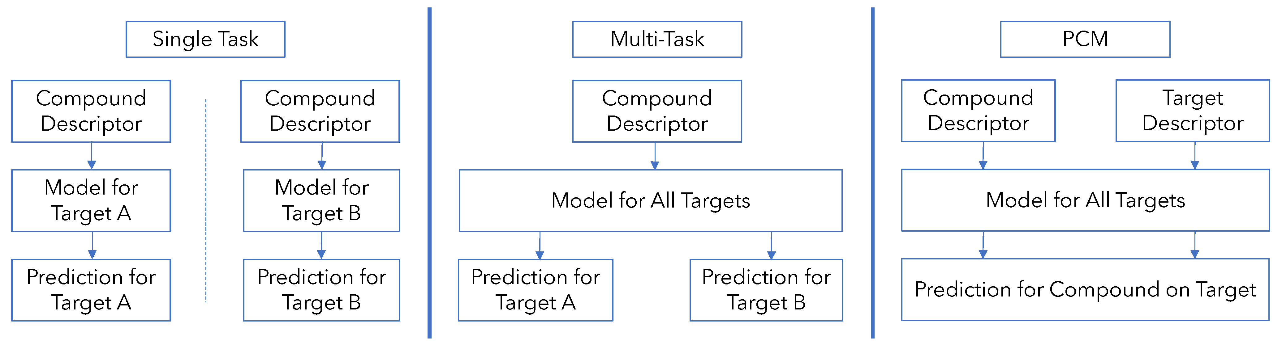
1. Introduction
2. Methods
2.1. Embeddings
2.2. Dataset and Evaluation
2.3. Development of Models
2.4. Model Quality Evaluation Metrics
3. Results and Discussion
4. Conclusions
Supplementary Materials
Author Contributions
Funding
Institutional Review Board Statement
Informed Consent Statement
Data Availability Statement
Acknowledgments
Conflicts of Interest
Appendix A. Data Splitting Implementation Details
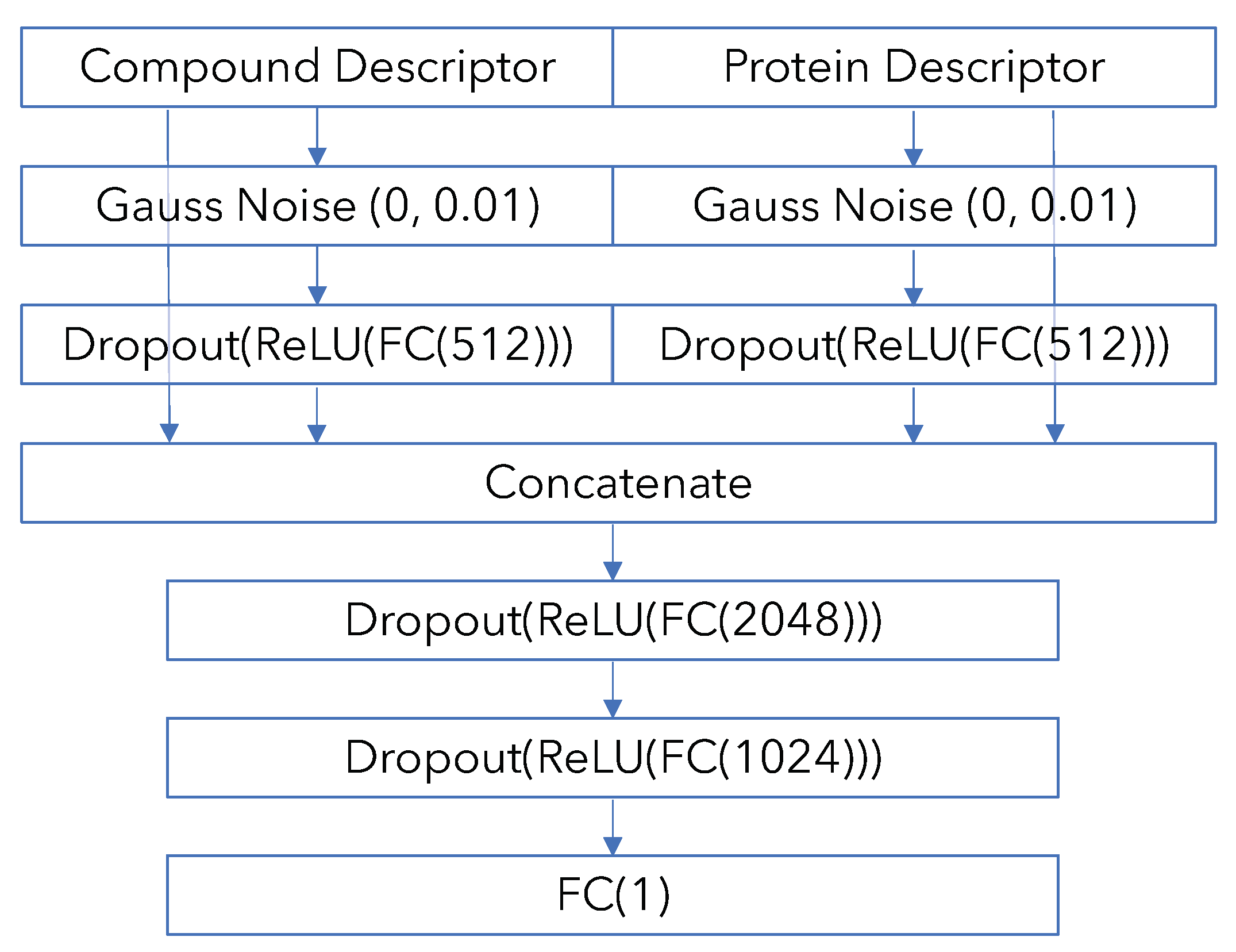
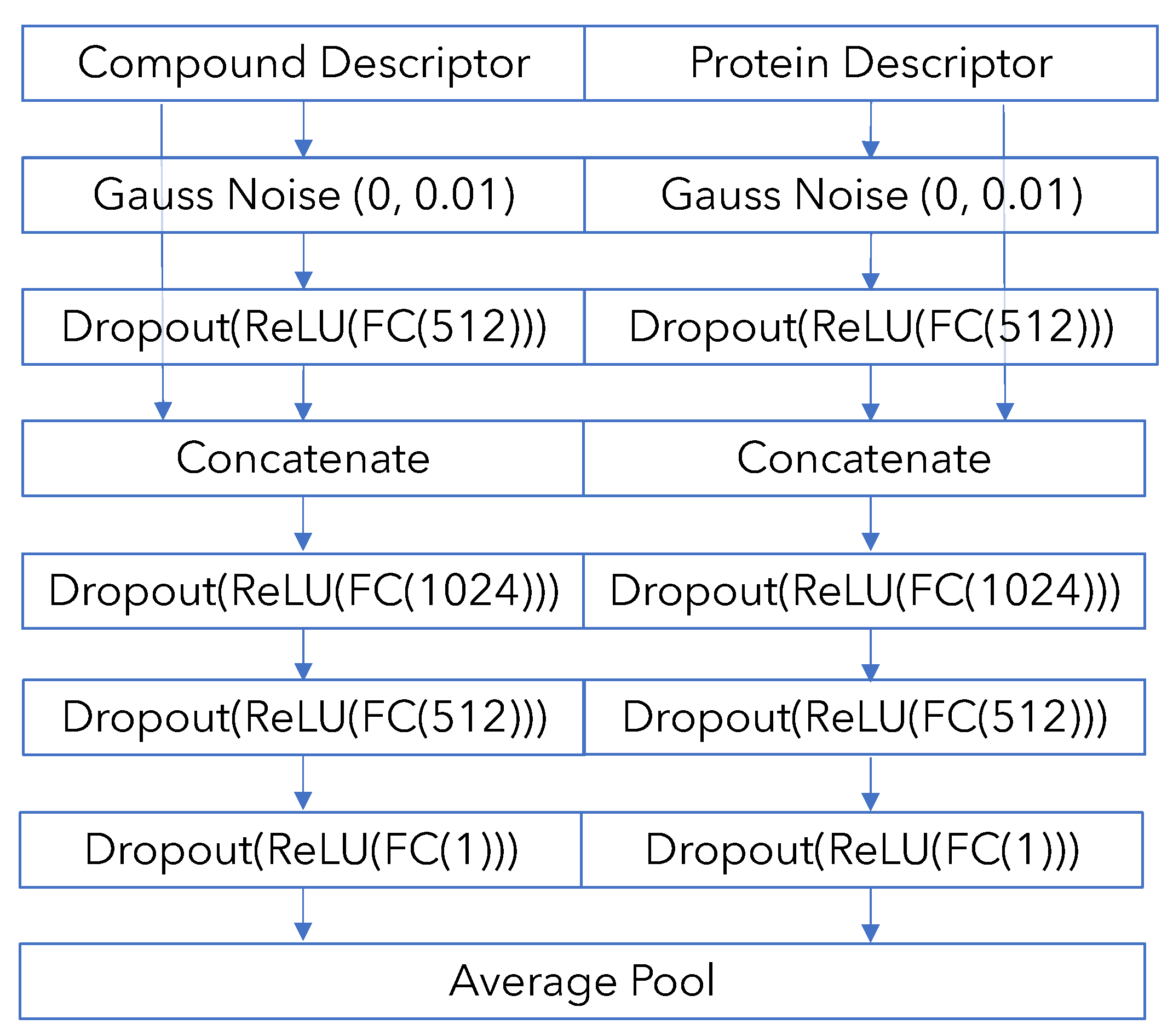
Appendix B. Model Architecture and Training Details


References
- Cortés-Ciriano, I.; Ain, Q.U.; Subramanian, V.; Lenselink, E.B.; Méndez-Lucio, O.; IJzerman, A.P.; Wohlfahrt, G.; Prusis, P.; Malliavin, T.E.; van Westen, G.J.; et al. Polypharmacology modelling using proteochemometrics (PCM): Recent methodological developments, applications to target families, and future prospects. MedChemComm 2015, 6, 24–50. [Google Scholar] [CrossRef]
- Van Westen, G.J.; Wegner, J.K.; IJzerman, A.P.; van Vlijmen, H.W.; Bender, A. Proteochemometric modeling as a tool to design selective compounds and for extrapolating to novel targets. MedChemComm 2011, 2, 16–30. [Google Scholar] [CrossRef]
- Lenselink, E.B.; Ten Dijke, N.; Bongers, B.; Papadatos, G.; Van Vlijmen, H.W.; Kowalczyk, W.; IJzerman, A.P.; Van Westen, G.J. Beyond the hype: Deep neural networks outperform established methods using a ChEMBL bioactivity benchmark set. J. Cheminform. 2017, 9, 45. [Google Scholar] [CrossRef]
- Cherkasov, A.; Muratov, E.N.; Fourches, D.; Varnek, A.; Baskin, I.I.; Cronin, M.; Dearden, J.; Gramatica, P.; Martin, Y.C.; Todeschini, R.; et al. QSAR modeling: Where have you been? Where are you going to? J. Med. Chem. 2014, 57, 4977–5010. [Google Scholar] [CrossRef]
- Caruana, R. Multitask learning. Mach. Learn. 1997, 28, 41–75. [Google Scholar] [CrossRef]
- Yuan, H.; Paskov, I.; Paskov, H.; González, A.J.; Leslie, C.S. Multitask learning improves prediction of cancer drug sensitivity. Sci. Rep. 2016, 6, 31619. [Google Scholar] [CrossRef] [PubMed]
- Simões, R.S.; Maltarollo, V.G.; Oliveira, P.R.; Honorio, K.M. Transfer and multi-task learning in QSAR modeling: Advances and challenges. Front. Pharmacol. 2018, 9, 74. [Google Scholar] [CrossRef]
- Dahl, G.E.; Jaitly, N.; Salakhutdinov, R. Multi-task neural networks for QSAR predictions. arXiv 2014, arXiv:1406.1231. [Google Scholar]
- Lima, A.N.; Philot, E.A.; Trossini, G.H.G.; Scott, L.P.B.; Maltarollo, V.G.; Honorio, K.M. Use of machine learning approaches for novel drug discovery. Expert Opin. Drug Discov. 2016, 11, 225–239. [Google Scholar] [CrossRef]
- Mitchell, J.B. Machine learning methods in chemoinformatics. Wiley Interdiscip. Rev. Comput. Mol. Sci. 2014, 4, 468–481. [Google Scholar] [CrossRef]
- Ballester, P.J.; Mitchell, J.B. A machine learning approach to predicting protein–ligand binding affinity with applications to molecular docking. Bioinformatics 2010, 26, 1169–1175. [Google Scholar] [CrossRef] [PubMed]
- Weill, N.; Valencia, C.; Gioria, S.; Villa, P.; Hibert, M.; Rognan, D. Identification of Nonpeptide Oxytocin Receptor Ligands by Receptor-Ligand Fingerprint Similarity Search. Mol. Inform. 2011, 30, 521–526. [Google Scholar] [CrossRef] [PubMed]
- Van Westen, G.J.; Swier, R.F.; Wegner, J.K.; IJzerman, A.P.; van Vlijmen, H.W.; Bender, A. Benchmarking of protein descriptor sets in proteochemometric modeling (part 1): Comparative study of 13 amino acid descriptor sets. J. Cheminform. 2013, 5, 41. [Google Scholar] [CrossRef] [PubMed]
- Shiraishi, A.; Niijima, S.; Brown, J.; Nakatsui, M.; Okuno, Y. Chemical Genomics Approach for GPCR–Ligand Interaction Prediction and Extraction of Ligand Binding Determinants. J. Chem. Inform. Model. 2013, 53, 1253–1262. [Google Scholar] [CrossRef]
- Cheng, T.; Li, Q.; Zhou, Z.; Wang, Y.; Bryant, S.H. Structure-based virtual screening for drug discovery: A problem-centric review. AAPS J. 2012, 14, 133–141. [Google Scholar] [CrossRef]
- Menden, M.P.; Iorio, F.; Garnett, M.; McDermott, U.; Benes, C.H.; Ballester, P.J.; Saez-Rodriguez, J. Machine learning prediction of cancer cell sensitivity to drugs based on genomic and chemical properties. PLoS ONE 2013, 8, e61318. [Google Scholar] [CrossRef]
- LeCun, Y.; Bengio, Y.; Hinton, G. Deep learning. Nature 2015, 521, 436. [Google Scholar]
- Schmidhuber, J. Deep learning in neural networks: An overview. Neural Netw. 2015, 61, 85–117. [Google Scholar] [CrossRef] [PubMed]
- Glen, R.C.; Bender, A.; Arnby, C.H.; Carlsson, L.; Boyer, S.; Smith, J. Circular fingerprints: Flexible molecular descriptors with applications from physical chemistry to ADME. IDrugs 2006, 9, 199. [Google Scholar]
- Rogers, D.; Hahn, M. Extended-connectivity fingerprints. J. Chem. Inf. Model. 2010, 50, 742–754. [Google Scholar] [CrossRef]
- Mauri, A.; Consonni, V.; Pavan, M.; Todeschini, R. Dragon software: An easy approach to molecular descriptor calculations. Match 2006, 56, 237–248. [Google Scholar]
- Yap, C.W. PaDEL-descriptor: An open source software to calculate molecular descriptors and fingerprints. J. Comput. Chem. 2011, 32, 1466–1474. [Google Scholar] [CrossRef]
- Sandberg, M.; Eriksson, L.; Jonsson, J.; Sjöström, M.; Wold, S. New chemical descriptors relevant for the design of biologically active peptides. A multivariate characterization of 87 amino acids. J. Med. Chem. 1998, 41, 2481–2491. [Google Scholar] [CrossRef]
- Lapins, M.; Worachartcheewan, A.; Spjuth, O.; Georgiev, V.; Prachayasittikul, V.; Nantasenamat, C.; Wikberg, J.E. A unified proteochemometric model for prediction of inhibition of cytochrome P450 isoforms. PLoS ONE 2013, 8, e66566. [Google Scholar] [CrossRef]
- Subramanian, V.; Prusis, P.; Xhaard, H.; Wohlfahrt, G. Predictive proteochemometric models for kinases derived from 3D protein field-based descriptors. MedChemComm 2016, 7, 1007–1015. [Google Scholar] [CrossRef][Green Version]
- Kruger, F.A.; Overington, J.P. Global analysis of small molecule binding to related protein targets. PLoS Comput. Biol. 2012, 8, e1002333. [Google Scholar] [CrossRef] [PubMed]
- Lapinsh, M.; Veiksina, S.; Uhlén, S.; Petrovska, R.; Mutule, I.; Mutulis, F.; Yahorava, S.; Prusis, P.; Wikberg, J.E. Proteochemometric mapping of the interaction of organic compounds with melanocortin receptor subtypes. Mol. Pharmacol. 2005, 67, 50–59. [Google Scholar] [PubMed]
- Nabu, S.; Nantasenamat, C.; Owasirikul, W.; Lawung, R.; Isarankura-Na-Ayudhya, C.; Lapins, M.; Wikberg, J.E.; Prachayasittikul, V. Proteochemometric model for predicting the inhibition of penicillin-binding proteins. J. Comput.-Aided Mol. Des. 2015, 29, 127–141. [Google Scholar] [CrossRef]
- Srivastava, N.; Mansimov, E.; Salakhudinov, R. Unsupervised learning of video representations using lstms. Int. Conf. Mach. Learn. 2015, 37, 843–852. [Google Scholar]
- Erhan, D.; Bengio, Y.; Courville, A.; Manzagol, P.A.; Vincent, P.; Bengio, S. Why does unsupervised pre-training help deep learning? J. Mach. Learn. Res. 2010, 11, 625–660. [Google Scholar]
- Mikolov, T.; Sutskever, I.; Chen, K.; Corrado, G.S.; Dean, J. Distributed representations of words and phrases and their compositionality. In Advances in Neural Information Processing Systems; MIT Press: Cambridge, MA, USA, 2013; pp. 3111–3119. [Google Scholar]
- Winter, R.; Montanari, F.; Noé, F.; Clevert, D.A. Learning continuous and data-driven molecular descriptors by translating equivalent chemical representations. Chem. Sci. 2019, 10, 1692–1701. [Google Scholar] [CrossRef] [PubMed]
- Fabian, B.; Edlich, T.; Gaspar, H.; Segler, M.; Meyers, J.; Fiscato, M.; Ahmed, M. Molecular representation learning with language models and domain-relevant auxiliary tasks. arXiv 2020, arXiv:2011.13230. [Google Scholar]
- Alley, E.C.; Khimulya, G.; Biswas, S.; AlQuraishi, M.; Church, G.M. Unified rational protein engineering with sequence-only deep representation learning. bioRxiv 2019, 589333. [Google Scholar] [CrossRef]
- Heinzinger, M.; Elnaggar, A.; Wang, Y.; Dallago, C.; Nechaev, D.; Matthes, F.; Rost, B. Modeling aspects of the language of life through transfer-learning protein sequences. BMC Bioinform. 2019, 20, 723. [Google Scholar]
- Rives, A.; Meier, J.; Sercu, T.; Goyal, S.; Lin, Z.; Liu, J.; Guo, D.; Ott, M.; Zitnick, C.L.; Ma, J.; et al. Biological structure and function emerge from scaling unsupervised learning to 250 million protein sequences. Proc. Natl. Acad. Sci. USA 2021, 118, e2016239118. [Google Scholar] [CrossRef]
- Krause, B.; Lu, L.; Murray, I.; Renals, S. Multiplicative LSTM for sequence modelling. arXiv 2016, arXiv:1609.07959. [Google Scholar]
- Vaswani, A.; Shazeer, N.; Parmar, N.; Uszkoreit, J.; Jones, L.; Gomez, A.N.; Kaiser, Ł.; Polosukhin, I. Attention is all you need. In Advances in Neural Information Processing Systems; MIT Press: Cambridge, MA, USA, 2017; pp. 5998–6008. [Google Scholar]
- Cho, K.; Van Merriënboer, B.; Gulcehre, C.; Bahdanau, D.; Bougares, F.; Schwenk, H.; Bengio, Y. Learning phrase representations using RNN encoder-decoder for statistical machine translation. arXiv 2014, arXiv:1406.1078. [Google Scholar]
- Hochreiter, S.; Schmidhuber, J. Long Short-Term Memory. Neural Comput. 1997, 9, 1735–1780. [Google Scholar] [CrossRef]
- Kim, P.; Winter, R.; Clevert, D.A. Deep Protein-Ligand Binding Prediction Using Unsupervised Learned Representations. ChemRxiv 2020. [Google Scholar] [CrossRef]
- Kingma, D.P.; Ba, J. Adam: A method for stochastic optimization. arXiv 2014, arXiv:1412.6980. [Google Scholar]
- Truchon, J.F.; Bayly, C.I. Evaluating virtual screening methods: Good and bad metrics for the “early recognition” problem. J. Chem. Inf. Model. 2007, 47, 488–508. [Google Scholar] [CrossRef] [PubMed]


| Marginal Performance | Model Info | |||||
|---|---|---|---|---|---|---|
| Random MCC | LCCO MCC | LPO MCC | Repr Size | # Params | Type | |
| CDDD | 0.610 | 0.483 | 0.309 | 512 | 26 M | GRU-Autoencoder |
| MolBert | 0.630 | 0.497 | 0.306 | 768 | 85 M | Transformer |
| UniRep | 0.649 | 0.498 | 0.306 | 256 | 1.8 M | m-LSTM |
| SeqVec | 0.591 | 0.481 | 0.317 | 1024 | 93 M | Stacked LSTM |
| ESM | 0.629 | 0.492 | 0.296 | 1280 | 650 M | Transformer |
| Random | LCCO | LPO | ||||
|---|---|---|---|---|---|---|
| MCC | BedROC | MCC | BedROC | MCC | BedROC | |
| CDDD + UniRep | 0.645 (0.004) | 0.979 (0.002) | 0.490 (0.061) | 0.941 (0.017) | 0.307 (0.031) | 0.847 (0.038) |
| CDDD + SeqVec | 0.575 (0.079) | 0.967 (0.012) | 0.475 (0.060) | 0.930 (0.021) | 0.322(0.028) | 0.851 (0.041) |
| CDDD + ESM | 0.609 (0.014) | 0.974 (0.003) | 0.484 (0.054) | 0.930 (0.023) | 0.297 (0.093) | 0.834 (0.093) |
| MolBert + UniRep | 0.654 (0.005) | 0.980 (0.002) | 0.505 (0.053) | 0.943 (0.018) | 0.312 (0.024) | 0.847 (0.040) |
| MolBert + SeqVec | 0.607 (0.030) | 0.973 (0.007) | 0.487 (0.062) | 0.938 (0.017) | 0.311 (0.035) | 0.842 (0.049) |
| MolBert + ESM | 0.630 (0.009) | 0.977 (0.002) | 0.499 (0.053) | 0.937 (0.022) | 0.294 (0.118) | 0.832 (0.090) |
| Handcrafted | 0.337 (0.003) | 0.819 (0.007) | 0.276 (0.024) | 0.753 (0.058) | 0.132 (0.051) | 0.655 (0.061) |
| MCC | BedROC | |
|---|---|---|
| CDDD + UniRep | 0.633 (0.021) | 0.931 (0.023) |
| CDDD + SeqVec | 0.626 (0.016) | 0.922 (0.022) |
| CDDD + ESM | 0.634 (0.023) | 0.927 (0.022) |
| MolBert + UniRep | 0.645 (0.013) | 0.936 (0.018) |
| MolBert + SeqVec | 0.639 (0.012) | 0.928 (0.021) |
| MolBert + ESM | 0.646 (0.021) | 0.932 (0.021) |
| Random | LCCO | LPO | |||||||
|---|---|---|---|---|---|---|---|---|---|
| No-Int | Full | % Imp | No-Int | Full | % Imp | No-Int | Full | % Imp | |
| CDDD + UniRep | 0.565 | 0.645 | 14.3 | 0.424 | 0.490 | 15.6 | 0.281 | 0.307 | 9.3 |
| CDDD + SeqVec | 0.548 | 0.575 | 4.9 | 0.411 | 0.475 | 15.6 | 0.287 | 0.322 | 12.2 |
| CDDD + ESM | 0.557 | 0.609 | 9.4 | 0.416 | 0.484 | 16.3 | 0.287 | 0.297 | 3.5 |
| MolBert + UniRep | 0.574 | 0.654 | 13.8 | 0.439 | 0.505 | 15.0 | 0.283 | 0.312 | 10.2 |
| MolBert + SeqVec | 0.558 | 0.607 | 8.7 | 0.430 | 0.487 | 13.3 | 0.290 | 0.311 | 7.2 |
| MolBert + ESM | 0.567 | 0.630 | 11.2 | 0.434 | 0.499 | 15.0 | 0.292 | 0.294 | 0.7 |
Publisher’s Note: MDPI stays neutral with regard to jurisdictional claims in published maps and institutional affiliations. |
© 2021 by the authors. Licensee MDPI, Basel, Switzerland. This article is an open access article distributed under the terms and conditions of the Creative Commons Attribution (CC BY) license (https://creativecommons.org/licenses/by/4.0/).
Share and Cite
Kim, P.T.; Winter, R.; Clevert, D.-A. Unsupervised Representation Learning for Proteochemometric Modeling. Int. J. Mol. Sci. 2021, 22, 12882. https://doi.org/10.3390/ijms222312882
Kim PT, Winter R, Clevert D-A. Unsupervised Representation Learning for Proteochemometric Modeling. International Journal of Molecular Sciences. 2021; 22(23):12882. https://doi.org/10.3390/ijms222312882
Chicago/Turabian StyleKim, Paul T., Robin Winter, and Djork-Arné Clevert. 2021. "Unsupervised Representation Learning for Proteochemometric Modeling" International Journal of Molecular Sciences 22, no. 23: 12882. https://doi.org/10.3390/ijms222312882
APA StyleKim, P. T., Winter, R., & Clevert, D.-A. (2021). Unsupervised Representation Learning for Proteochemometric Modeling. International Journal of Molecular Sciences, 22(23), 12882. https://doi.org/10.3390/ijms222312882