
Mathematical Modelling of p53 Signalling during DNA Damage Response: A Survey


Abstract
1. Introduction
2. Mathematical Modelling of p53
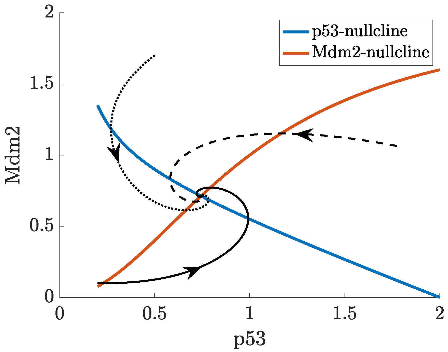
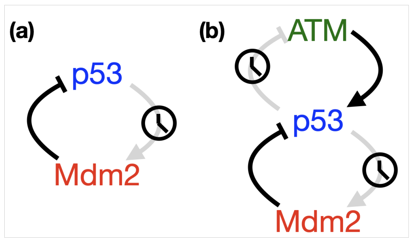
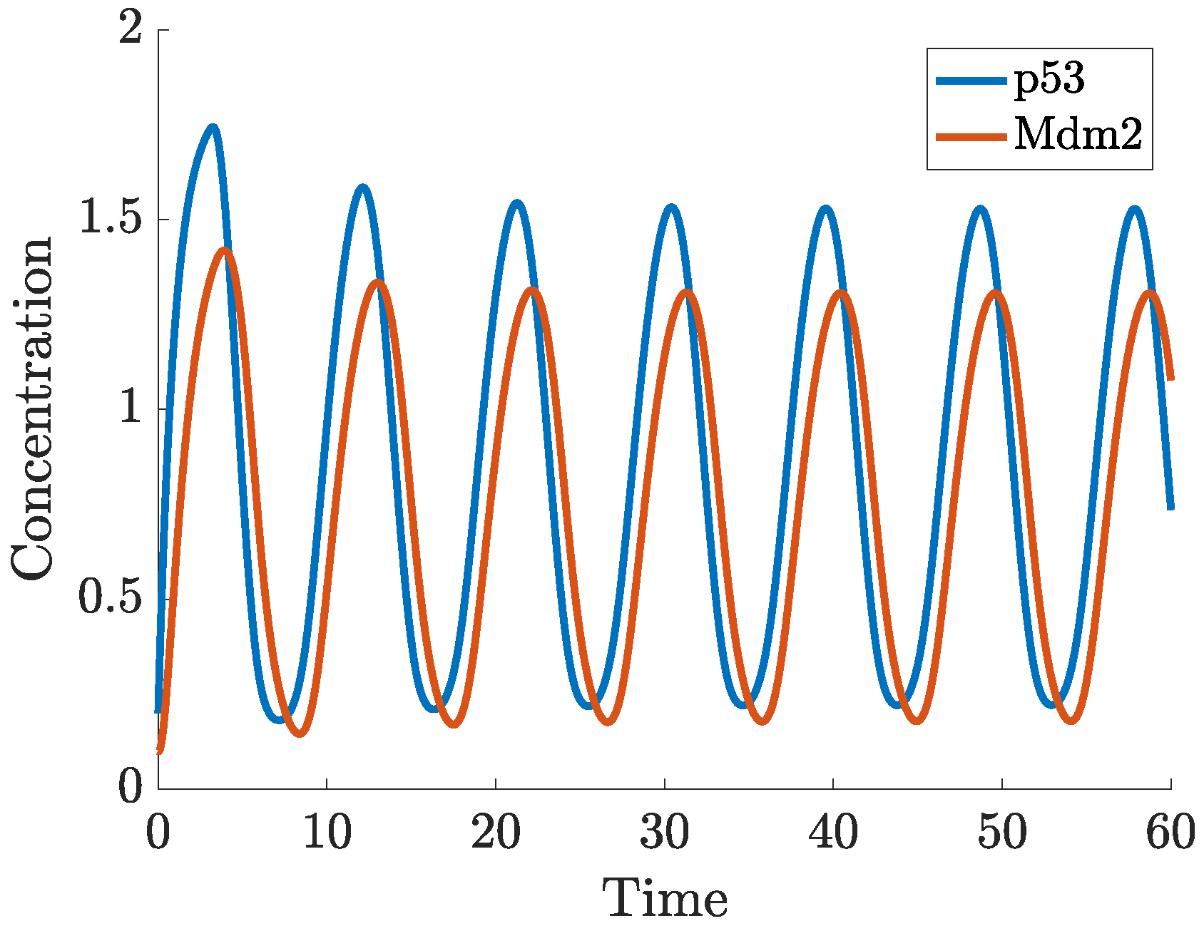
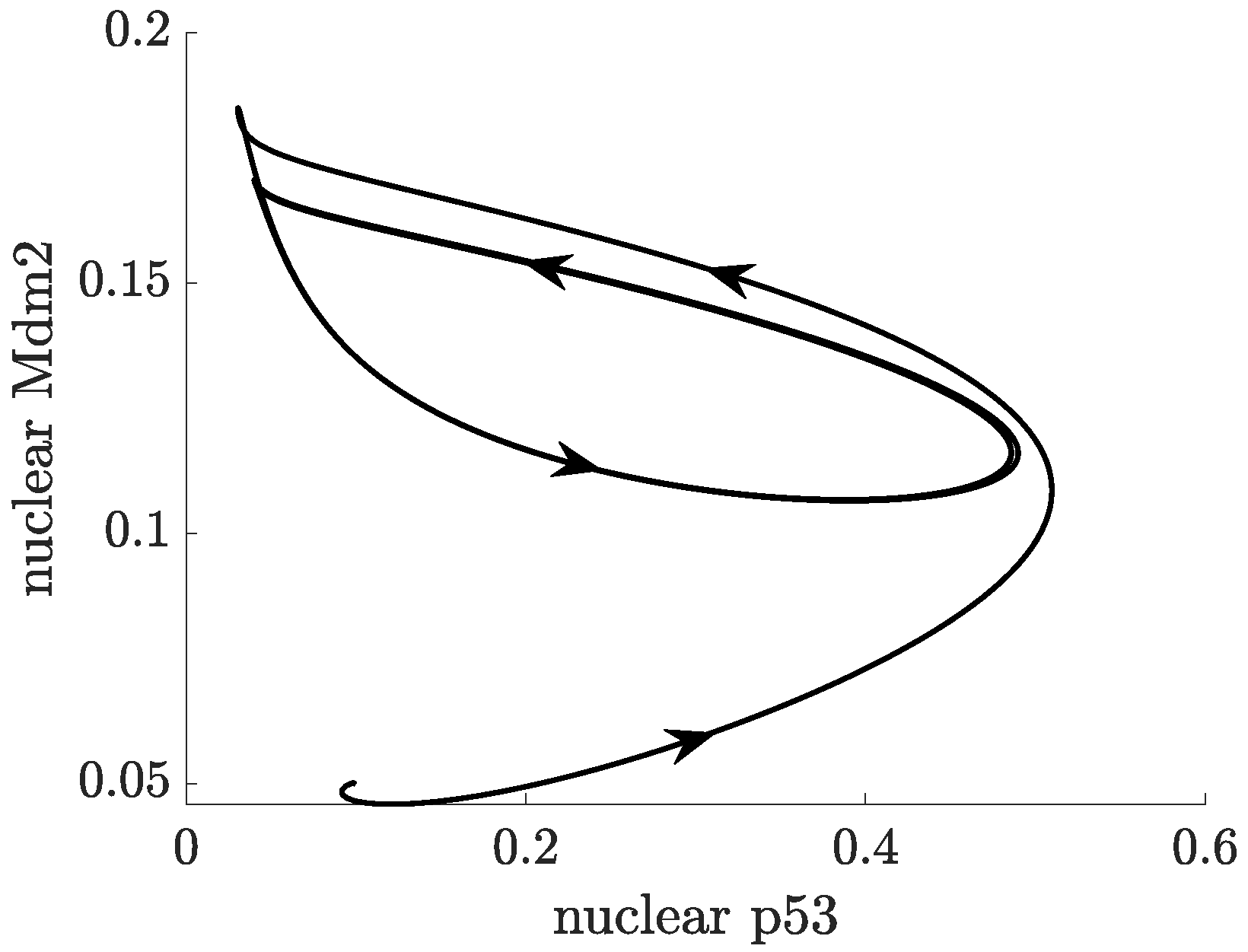
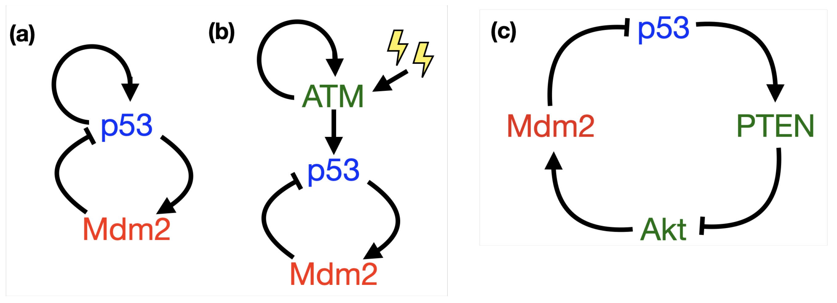
- p53-Mdm2 negative feedback loop
2.1. Time Delays in p53 Modelling
- p53-Mdm2 negative feedback loop with delay
2.2. Incorporating Diffusion in p53 Modelling
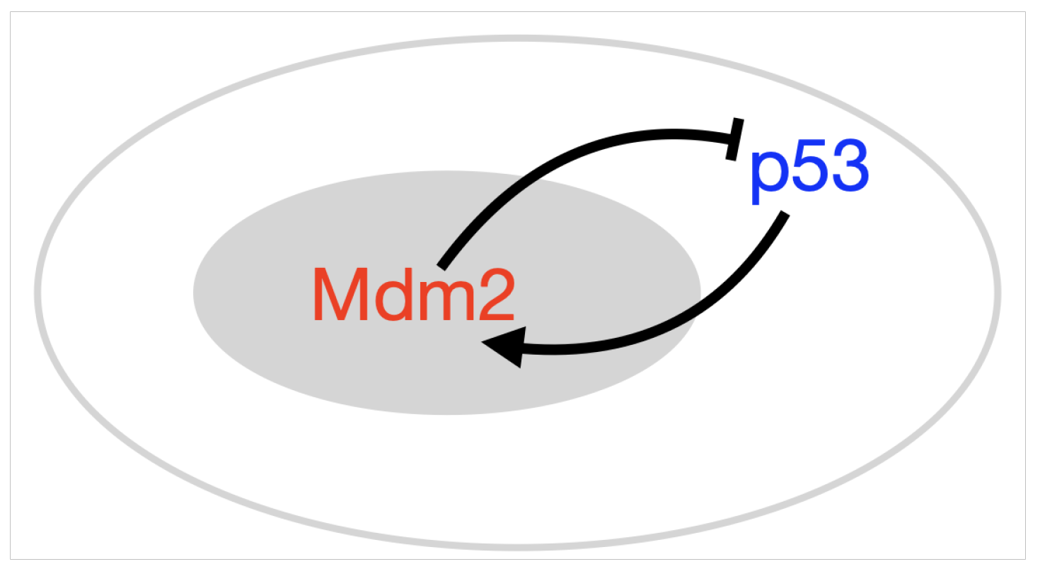
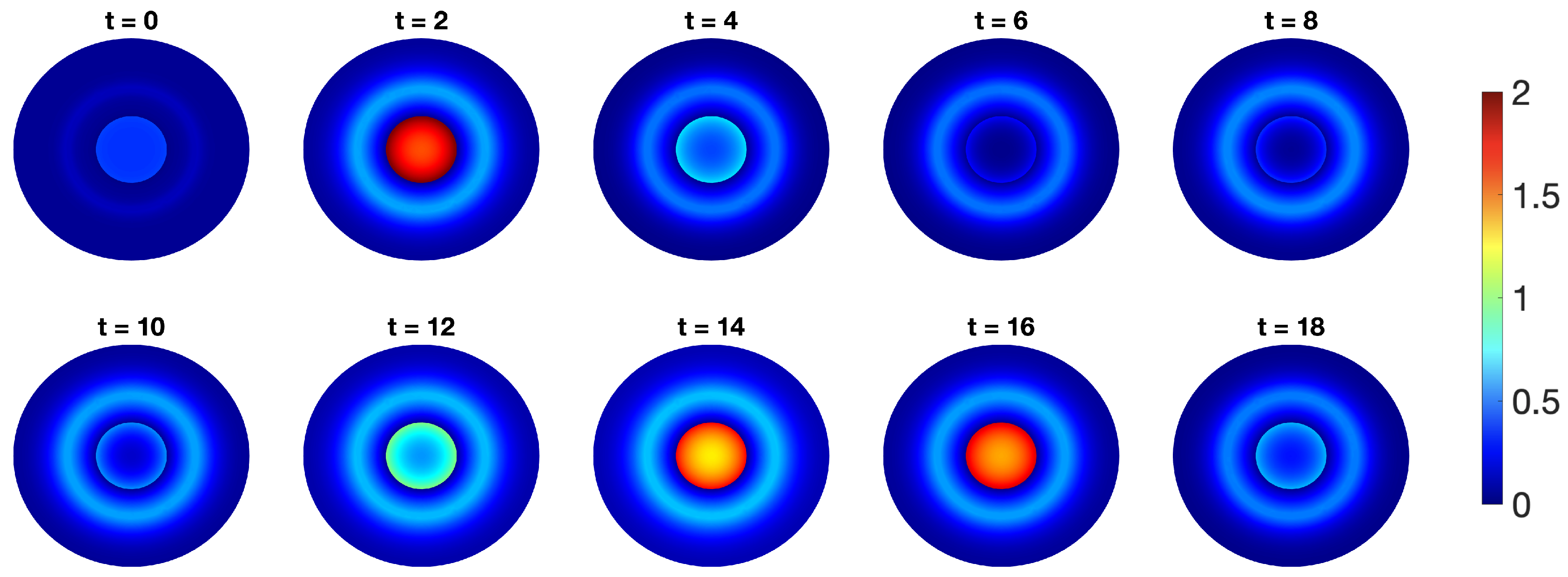
- p53-Mdm2 negative feedback loop with diffusion
2.3. Positive Feedback in p53 Modelling
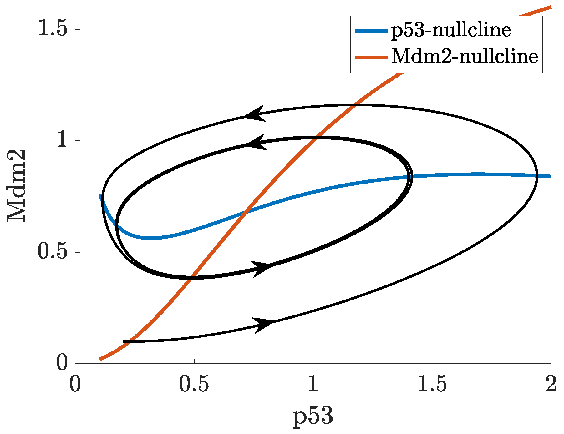
- p53-Mdm2 negative feedback loop with a positive feedback
3. Interplay between Experiments and Modelling
3.1. It All Started with Galit Lahav
3.2. Mathematical Models Drive New Insights into p53 Signalling
3.3. Application of p53 Modelling in Cancer Treatment
4. Conclusions
Funding
Acknowledgments
Conflicts of Interest
Appendix A. Parameters and Vector Fields for Models (1)–(4)
| Model | Parameters |
| Negative feedback model (1) | ; ; ; ; ; ; |
| Time delay model (2) | ; ; ; ; ; ; ; |
| Spatial model (3) | *; ; ; ; ; ; ; ; ; ; permeability for x, y and z is set to 10 |
| Positive feedback model (4) | ; ; ; ; ; ; ; ; |
| * The synthesis rate of p53, , in the spatial model is the rate at which new p53 molecules are produced in the whole cell per a unit of time. | |

Appendix B. A Novel Model for p53

References
- Davidson, E.H.; Peter, I.S. Chapter 2—Gene Regulatory Networks. In Genomic Control Process; Davidson, E.H., Peter, I.S., Eds.; Oxford Academic Press: Oxford, UK, 2015; pp. 41–77. [Google Scholar]
- Greenblatt, M.S.; Bennett, W.P.; Hollstein, M.; Harris, C.C. Mutations in the p53 tumor suppressor gene: Clues to cancer etiology and molecular pathogenesis. Cancer Res. 1994, 54, 4855–4878. [Google Scholar]
- Gottlieb, T.M.; Oren, M. p53 in growth control and neoplasia. Biochim. Biophys. Acta Rev. Cancer 1996, 1287, 77–102. [Google Scholar] [CrossRef]
- Hainaut, P.; Hernandez, T.; Robinson, A.; Rodriguez-Tome, P.; Flores, T.; Hollstein, M.; Harris, C.; Montesano, R. IARC Database of p53 gene mutations in human tumors and cell lines: Updated compilation, revised formats and new visualisation tools. Nucleic Acids Res. 1998, 26, 205–213. [Google Scholar] [CrossRef]
- Bennett, W.P.; Hussain, S.P.; Vahakangas, K.H.; Khan, M.A.; Shields, P.G.; Harris, C.C. Molecular epidemiology of human cancer risk: Gene-environment interactions and p53 mutation spectrum in human lung cancer. J. Pathol. 1999, 187, 8–18. [Google Scholar] [CrossRef]
- Vousden, K.H.; Lane, D.P. p53 in health and disease. Nat. Mol. Cell Biol. 2007, 8, 275–283. [Google Scholar] [CrossRef]
- Malkin, D.; Li, F.P.; Strong, L.C.; Fraumeni, J.F.; Nelson, C.E.; Kim, D.H.; Kassel, J.; Gryka, M.A.; Bischoff, F.Z.; Tainsky, M.A.; et al. Germ line p53 mutations in a familial syndrome of breast cancer, sarcomas, and other neoplasms. Science 1990, 250, 1233–1238. [Google Scholar] [CrossRef] [PubMed]
- Vogelstein, B. Cancer. A deadly inheritance. Nature 1990, 348, 681–682. [Google Scholar] [CrossRef] [PubMed]
- Levine, A.J. p53, the cellular gatekeeper for growth and division. Cell 1997, 88, 323–331. [Google Scholar] [CrossRef]
- Agarwal, M.L.; Taylor, W.R.; Chernov, M.V.; Chernova, O.B.; Stark, G.R. The p53 network. J. Biol. Chem. 1998, 273, 1–4. [Google Scholar] [CrossRef] [PubMed]
- Vogelstein, B.; Lane, D.; Levine, A.J. Surfing the p53 network. Nature 2000, 408, 307–310. [Google Scholar] [CrossRef] [PubMed]
- Lane, D.P. p53, guardian of the genome. Nature 1992, 358, 15–16. [Google Scholar] [CrossRef]
- Horn, H.F.; Vousden, K.H. Coping with stress: Multiple ways to activate p53. Oncogene 2007, 26, 1306–1316. [Google Scholar] [CrossRef]
- Unger, T.; Juven-Gershon, T.; Moallem, E.; Berger, M.; Vogt Sionov, R.; Lozano, G.; Oren, M.; Haupt, Y. Critical role for Ser20 of human p53 in the negative regulation of p53 by Mdm2. EMBO J. 1999, 18, 1805–1814. [Google Scholar] [CrossRef]
- Batchelor, E.; Loewer, A.; Mock, C.; Lahav, G. Stimulus-dependent dynamics of p53 in single cells. Mol. Syst. Biol. 2011, 7, 8. [Google Scholar] [CrossRef] [PubMed]
- Purvis, J.E.; Karhohs, K.W.; Mock, C.; Batchelor, E.; Loewer, A.; Lahav, G. p53 dynamics control cell fate. Science 2012, 336, 1440–1444. [Google Scholar] [CrossRef] [PubMed]
- Hirata, H.; Yoshiura, S.; Ohtsuka, T.; Bessho, Y.; Harada, T.; Yoshikawa, K.; Kageyama, R. Oscillatory expression of the bHLH factor Hes1 regulated by a negative feedback loop. Science 2002, 298, 840–843. [Google Scholar] [CrossRef] [PubMed]
- Lev Bar-Or, R.; Maya, R.; Segel, L.A.; Alon, U.; Levine, A.J.; Oren, M. Generation of oscillations by the p53-Mdm2 feedback loop: A theoretical and experimental study. Proc. Natl. Acad. Sci. USA 2000, 97, 11250–11255. [Google Scholar] [CrossRef]
- Geva-Zatorsky, N.; Rosenfeld, N.; Itzkovitz, S.; Milo, R.; Sigal, A.; Dekel, E.; Yarnitzky, T.; Liron, Y.; Polak, P.; Lahav, G.; et al. Oscillations and variability in the p53 system. Mol. Syst. Biol. 2006, 2, 2006-0033. [Google Scholar] [CrossRef]
- Lahav, G.; Rosenfeld, N.; Sigal, A.; Geva-Zatorsky, N.; Levine, A.J.; Elowitz, M.B.; Alon, U. Dynamics of the p53-Mdm2 feedback loop in individual cells. Nat. Genet. 2004, 36, 147–150. [Google Scholar] [CrossRef]
- Loewer, A.; Karanam, K.; Mock, C.; Lahav, G. The p53 response in single cells is linearly correlated to the number of DNA breaks without a distinct threshold. BMC Biol. 2013, 11, 13. [Google Scholar] [CrossRef]
- Hamstra, D.A.; Bhojani, M.S.; Griffin, L.B.; Laxman, B.; Ross, B.D.; Rehemtulla, A. Real-time Evaluation of p53 Oscillatory Behavior In vivo Using Bioluminescent Imaging. Cancer Res. 2006, 66, 7482–7489. [Google Scholar] [CrossRef]
- Haupt, Y.; Maya, R.; Kazaz, A.; Oren, M. Mdm2 promotes the rapid degradation of p53. Nature 1997, 387, 296–299. [Google Scholar] [CrossRef]
- Oliner, J.D.; Pietenpol, J.A.; Thiagalingam, S.; Gyuris, J.; Kinzler, K.W.; Vogelstein, B. Oncoprotein MDM2 conceals the activation domain of tumour suppressor p53. Nature 1993, 362, 857–860. [Google Scholar] [CrossRef]
- Mendrysa, S.M.; Perry, M.E. The p53 tumor suppressor protein does not regulate expression of is own inhibitor, MDM2, except under conditions of stress. Mol. Cell. Biol. 2000, 20, 2023–2030. [Google Scholar] [CrossRef]
- Goodwin, B.C. Temporal Organization in Cells; A Dynamic Theory of Cellular Control Processes; Academic Press: London, UK, 1963; p. 184. [Google Scholar]
- Goodwin, B.C. Oscillatory behaviour in enzymatic control processes. Adv. Enzyme Regul. 1965, 3, 425–428. [Google Scholar] [CrossRef]
- Griffith, J.S. Mathematics of cellular control processes. I. negative feedback to one gene. J. Theor. Biol. 1968, 20, 202–208. [Google Scholar] [CrossRef]
- Jensen, M.H.; Sneppen, J.; Tiana, G. Sustained oscillations and time delays in gene expression of protein Hes1. FEBS Lett. 2003, 541, 176–177. [Google Scholar] [CrossRef]
- Lewis, J. Autoinhibition with Transcriptional Delay: A Simple Mechanism for the Zebrafish Somitogenesis Oscillator. Curr. Biol. 2003, 13, 1398–1408. [Google Scholar] [CrossRef]
- Monk, N.A.M. Oscillatory expression of Hes1, p53, and NF-κB driven by transcriptional time delays. Curr. Biol. 2003, 13, 1409–1413. [Google Scholar] [CrossRef]
- Bernard, S.; Čajavec, B.; Pujo-Menjouet, L.; Mackey, M.C.; Herzel, H. Modeling transcriptional feedback loops: The role of Gro/TLE1 in Hes1 oscillations. Philos. Trans. A Math. Phys. Eng. Sci. 2006, 15, 1155–1170. [Google Scholar]
- Barrio, M.; Burrage, K.; Leier, A.; Tian, T. Oscillatory regulation of Hes1: Discrete stochastic delay modelling and simulation. PLoS Comput. Biol. 2006, 2, e117. [Google Scholar] [CrossRef]
- Bodnar, M.; Bartłlomiejczyk, A. Stability of delay induced oscillations in gene expression of Hes1 protein model. Nonlinear Anal. Real World Appl. 2012, 13, 2227–2239. [Google Scholar] [CrossRef]
- Parmar, K.; Blyuss, K.B.; Kyrychko, Y.N.; Hogan, S.J. Time-Delayed Models of Gene Regulatory Networks. Comput. Math. Methods Med. 2015, 2015, 347273. [Google Scholar] [CrossRef]
- Yu, W.T.; Tang, J.; Ma, J.; Luo, J.M.; Yang, X.Q. Damped oscillations in a multiple delayed feedback NF-κB signaling module. Eur. Biophys. J. 2015, 44, 677–684. [Google Scholar] [CrossRef]
- Bodnar, M. Distributed delays in Hes1 gene expression model. Discret. Contin. Dyn. Syst. B 2019, 24, 2125–2147. [Google Scholar] [CrossRef]
- Liu, L.; Yan, F.; Liu, H. Oscillation expression of NF-κB driven by transcription and translation time delays. IEEE Trans. NanoBiosci. 2020, 19, 35–47. [Google Scholar] [CrossRef]
- Smolen, P.; Baxter, D.A.; Byrne, J.H. Mathematical modeling of gene networks. Neuron 2000, 26, 567–580. [Google Scholar] [CrossRef]
- Xiao, M.; Cao, J. Genetic oscillation deduced from Hopf bifurcation in a genetic regulatory network with delays. Math. Biosci. 2008, 215, 55–63. [Google Scholar] [CrossRef]
- Wan, A.; Zou, X. Hopf bifurcation analysis for a model of genetic regulatory system with delay. J. Math. Anal. Appl. 2009, 356, 464–476. [Google Scholar] [CrossRef][Green Version]
- Wang, K.; Wang, L.; Teng, Z.; Jiang, H. Stability and bifurcation of genetic regulatory networks with delays. Neurocomputing 2010, 73, 2882–2892. [Google Scholar] [CrossRef]
- Bodnar, M.; Foryś, U.; Poleszczuk, J. Analysis of biochemical reactions models with delays. J. Math. Anal. Appl. 2011, 376, 74–83. [Google Scholar] [CrossRef]
- Cao, J.; Jiang, H. Hopf bifurcation analysis for a model of single genetic negative feedback autoregulatory system with delay. Neurocumputing 2013, 99, 381–389. [Google Scholar] [CrossRef]
- Xiao, M.; Zheng, W.X.; Cao, J. Stability and bifurcation of genetic regulatory networks with small RNAs and multiple delays. Int. J. Comput. Math. 2014, 91, 907–927. [Google Scholar] [CrossRef]
- Ahmed, A.; Verriest, E.I. Modeling & analysis of gene expression as a nonlinear feedback problem with state-dependent delay. IFAC-PapersOnLine 2017, 50, 12679–12684. [Google Scholar]
- Pei, L.; Wang, S.; Wiercigroch, M. Analysis of Hopf bifurcations in differential equations with state-dependent delays via multiple scales method. ZAMM J. Appl. Math. Mech. 2018, 98, 789–801. [Google Scholar] [CrossRef]
- Pei, L.; Wang, S. Double Hopf bifurcation of differential equation with linearly state-dependent delays via MMS. Appl. Math. Comput. 2019, 341, 256–276. [Google Scholar] [CrossRef]
- Wang, S.; Pei, L. Complex dynamics and periodic oscillation mechanism in two novel gene expression models with state-dependent delays. Int. J. Bifurc. Chaos 2021, 31, 2150002. [Google Scholar] [CrossRef]
- Tyson, J.J.; Othmer, H.G. The dynamics of feedback control circuits in biochemical pathways. In Progress in Theoretical Biology; Academic Press: New York, NY, USA, 1978; Volume 5, pp. 1–62. [Google Scholar]
- Keller, A.D. Specifying epigenetic states with autoregulatory transcription factors. J. Theor. Biol. 1994, 170, 175–181. [Google Scholar] [CrossRef] [PubMed]
- Henrich, R.; Schuster, S. The Regulation of Cellular Systems; Chapman & Hall: New York, NY, USA, 1996. [Google Scholar]
- Gouzé, J. Positive and Negative Circuits in Dynamical Systems. J. Biol. Syst. 1998, 6, 11–15. [Google Scholar] [CrossRef]
- Snoussi, E.H. Necessary conditions for multistationarity and stable periodicity. J. Biol. Syst. 1998, 6, 3–9. [Google Scholar] [CrossRef]
- Smolen, P.; Baxter, D.A.; Byrne, J.H. Modeling circadian oscillations with interlocking positive and negative feedback loops. J. Neurosci. 2001, 21, 6644–6656. [Google Scholar] [CrossRef] [PubMed]
- Pfeuty, B.; Kaneko, K. The combination of positive and negative feedback loops confers exquisite flexibility to biochemical switches. Phys. Biol. 2009, 6, 046013. [Google Scholar] [CrossRef]
- Mahaffy, J.M.; Pao, C.V. Models of genetic control by repression with time delays and spatial effects. J. Math. Biol. 1984, 20, 39–57. [Google Scholar] [CrossRef]
- Busenberg, S.; Mahaffy, J.M. Interaction of spatial diffusion and delays in models of genetic control by repression. J. Math. Biol. 1985, 22, 313–333. [Google Scholar] [CrossRef]
- Mahaffy, J.M. Genetic control models with diffusion and delays. Math. Biosci. 1988, 90, 519–533. [Google Scholar] [CrossRef]
- Smolen, P.; Baxter, D.A.; Byrne, J.H. Effects of macromolecular transport and stochastic fluctuations on the dynamics of genetic regulatory systems. Am. J. Physiol. 1999, 277, C777–C790. [Google Scholar] [CrossRef] [PubMed]
- Sturrock, M.; Hellander, A.; Matzavinos, A.; Chaplain, M.A.J. Spatial stochastic modelling of the Hes1 gene regulatory network: Intrinsic noise can explain heterogeneity in embryonic stem cell differentiation. J. R. Soc. Interface 2013, 10, 20120988. [Google Scholar] [CrossRef]
- Chaplain, M.A.J.; Ptashnyk, M.; Sturrock, M. Hopf bifurcation in a gene regulatory network model: Molecular movement causes oscillations. Math. Model. Methods Appl. Sci. 2015, 25, 1179–1215. [Google Scholar] [CrossRef]
- Sturrock, M.; Murray, P.J.; Matzavinos, A.; Chaplain, M.A.J. Mean field analysis of a spatial stochastic model of a gene regulatory network. J. Math. Biol. 2015, 71, 921–959. [Google Scholar] [CrossRef]
- Macnamara, C.K.; Chaplain, M.A.J. Diffusion driven oscillations in gene regulatory networks. J. Theor. Biol. 2016, 407, 51–70. [Google Scholar] [CrossRef][Green Version]
- Macnamara, C.K.; Chaplain, M.A.J. Spatio-temporal models of synthetic genetic oscillators. Math. Biol. Eng. 2017, 14, 249–262. [Google Scholar] [CrossRef][Green Version]
- Macnamara, C.K.; Mitchell, E.; Chaplain, M.A.J. Spatial-Stochastic modelling of synthetic gene regulatory networks. J. Theor. Biol. 2019, 468, 27–44. [Google Scholar] [CrossRef]
- Novák, B.; Tyson, J.J. Design principles of biochemical oscillators. Nat. Rev. Mol. Cell Biol. 2008, 9, 981–991. [Google Scholar] [CrossRef] [PubMed]
- Alon, U. An Introduction to Systems Biology: Design Principles of Biological Circuits, 2nd ed.; CRC Press: Boca Raton, FL, USA, 2019. [Google Scholar]
- Available online: https://github.com/janelias1/p53-in-DNA-damage (accessed on 31 August 2021).
- Hirsch, M.W.; Smale, S.; Devaney, R.L. Differential Equations, Dynamical Systems, and an Introduction to Chaos, 3rd ed.; Academic Press: Boston, MA, USA, 2013. [Google Scholar]
- Uptain, S.M.; Kane, C.M.; Chamberlin, M.J. Basic mechanisms of transcript elongation and its regulation. Annu. Rev. Biochem. 1997, 66, 117–172. [Google Scholar] [CrossRef]
- Audibert, A.; Weil, D.; Dautry, F. In vivo kinetics of mRNA splicing and transport in mammalian cells. Mol. Cell. Biol. 2002, 22, 6706–6718. [Google Scholar] [CrossRef] [PubMed]
- Bentley, D. The mRNA assembly line: Transcription and processing machines in the same factory. Curr. Opin. Cell Biol. 2002, 14, 336–342. [Google Scholar] [CrossRef]
- Mihalaş, G.I.; Simon, Z.; Balea, G.; Popa, E. Possible oscillatory behaviour in p53-mdm2 interaction computer simulation. J. Biol. Syst. 2000, 8, 21–29. [Google Scholar] [CrossRef]
- Tiana, G.; Jensen, M.H.; Sneppen, K. Time delay as a key to apoptosis induction in the p53 network. Eur. Phys. J. 2002, 29, 135–140. [Google Scholar] [CrossRef]
- Ogunnaike, B.A. Elucidating the digital control mechanism for DNA damage repair with the p53-Mdm2 system: Single cell data analysis and ensemble modelling. J. R. Soc. Interface 2006, 3, 175–184. [Google Scholar] [CrossRef]
- Yan, S.; Zhuo, Y. A unified model for studying DNA damage-induced p53–Mdm2 interaction. Phys. D Nonlinear Phenom. 2006, 220, 157–162. [Google Scholar] [CrossRef]
- Bottani, S.; Grammaticos, B. Analysis of a minimal model for p53 oscillations. J. Theor. Biol. 2007, 249, 235–245. [Google Scholar] [CrossRef] [PubMed]
- Tiana, G.; Krishna, S.; Pigolotti, S.; Jensen, M.H.; Sneppen, K. Oscillations and temporal signalling in cells. Phys. Biol. 2007, 4, R1–R17. [Google Scholar] [CrossRef] [PubMed]
- Tyson, J.J.; Chen, K.C.; Novak, B. Sniffers, buzzers, toggles and blinkers: Dynamics of regulatory and signaling pathways in the cell. Curr. Opin. Cell Biol. 2003, 15, 221–231. [Google Scholar] [CrossRef]
- Mihalaş, G.I.; Neamţu, M.; Opriş, D.; Horhat, R.F. A dynamic P53-MDM2 model with time delay. Chaos Solitons Fractals 2006, 30, 936–945. [Google Scholar] [CrossRef]
- Batchelor, E.; Mock, C.S.; Bhan, I.; Loewer, A.; Lahav, G. Recurrent initiation: A mechanism for triggering p53 pulses in response to DNA damage. Mol. Cell 2008, 30, 277–289. [Google Scholar] [CrossRef]
- Wang, C.; Liu, H.; Zhou, J. Contribution of time delays to p53 oscillation in DNA damage response. IET Syst. Biol. 2019, 13, 180–185. [Google Scholar] [CrossRef]
- Wang, D.; Liu, N.; Yang, H.; Yang, L. Theoretical analysis of the delay on the p53 micronetwork. Adv. Differ. Equs. 2020, 2020, 340. [Google Scholar] [CrossRef]
- Rateitschak, K.; Wolkenhauer, O. Intracellular delay limits cyclic changes in gene expression. Math. Biosci. 2006, 205, 163–179. [Google Scholar] [CrossRef]
- Horhat, R.F.; Neamtu, M.; Mircea, G. Mathematical models and numerical simulations for the p53-Mdm2 network. Appl. Sci. 2008, 10, 94–106. [Google Scholar]
- Horhat, R.F.; Neamtu, M.; Opris, D. The qualitative analysis for a differential system of the P53-Mdm2 interaction with delay kernel. In Proceedings of the 1st WSEAS International Conference on Biomedical Electronics and Biomedical Informatics, BEBI’08, Rhodes, Greece, 20–22 August 2008; pp. 208–214. [Google Scholar]
- Gordon, K.E.; van Leeuwen, I.M.M.; Lain, S.; Chaplain, M.A.J. Spatio-temporal modelling of the p53-Mdm2 oscillatory system. Math. Model. Nat. Phenom 2009, 4, 97–116. [Google Scholar] [CrossRef]
- Sturrock, M.; Terry, A.J.; Xirodimas, D.P.; Thompson, A.M.; Chaplain, M.A.J. Spatio-temporal modelling of the Hes1 and p53-Mdm2 intracellular signalling pathways. J. Theor. Biol. 2011, 273, 15–31. [Google Scholar] [CrossRef]
- Sturrock, M.; Terry, A.J.; Xirodimas, D.P.; Thompson, A.M.; Chaplain, M.A.J. Influence of the nuclear membrane, active transport, and cell shape on the Hes1 and p53-Mdm2 pathways: Insights from spatio-temporal modelling. Bull. Math. Biol. 2012, 74, 1531–1579. [Google Scholar] [CrossRef]
- Dimitrio, L.; Clairambault, J.; Natalini, R. A spatial physiological model for p53 intracellular dynamics. J. Theor. Biol. 2013, 316, 9–24. [Google Scholar] [CrossRef] [PubMed][Green Version]
- Eliaš, J.; Dimitrio, L.; Clairambault, J.; Natalini, R. The p53 protein and its molecular network: Modelling a missing link between DNA damage and cell fate. BBA Proteins Proteom. 2014, 1844, 232–247. [Google Scholar] [CrossRef]
- Paull, T.T.; Lee, J.H. The Mre11/Rad50/Nbs1 Complex and Its Role as a DNA Double-Strand Break Sensor for ATM. Cell Cycle 2005, 4, 737–740. [Google Scholar] [CrossRef] [PubMed]
- Bakkenist, C.J.; Kastan, M.B. DNA damage activates ATM through intermolecular autophosphorylation and dimer dissociation through intermolecular autophosphorylation and dimer dissociation. Nature 2003, 421, 499–506. [Google Scholar] [CrossRef]
- Eliaš, J.; Clairambault, J. Reaction-diffusion systems for spatio-temporal intracellular protein networks: A beginner’s guide with two examples. Comp. Struct. Biotechnol. J. 2014, 10, 14–22. [Google Scholar] [CrossRef] [PubMed]
- Eliaš, J.; Dimitrio, L.; Clairambault, J.; Natalini, R. Modelling p53 dynamics in single cells: Physiologically based ODE and reaction-diffusion PDE models. Phys. Biol. 2014, 11, 045001. [Google Scholar] [CrossRef]
- Eliaš, J. Positive effect of Mdm2 on p53 expression explains excitability of p53 in response to DNA damage. J. Theor. Biol. 2017, 418, 94–104. [Google Scholar] [CrossRef]
- Gajjar, M.; Candeias, M.M.; Malbert-Colas, L.; Mazars, A.; Fujita, J.; Olivares-Illana, V.; Fåhraeus, R. The p53 mRNA-Mdm2 interaction controls Mdm2 nuclear trafficking and is required for p53 activation following DNAdamage. Cancer Cell 2012, 21, 25–35. [Google Scholar] [CrossRef]
- Loewer, A.; Batchelor, E.; Gaglia, G.; Lahav, G. Basal Dynamics of p53 Reveal Transcriptionally Attenuated Pulses in Cycling Cells. Cell 2010, 142, 89–100. [Google Scholar] [CrossRef]
- Ciliberto, A.; Novák, B.; Tyson, J.J. Steady States and Oscillations in the p53/Mdm2 Network. Cell Cycle 2005, 4, 488–493. [Google Scholar] [CrossRef] [PubMed]
- Zhang, T.; Brazhnik, P.; Tyson, J.J. Exploring mechanisms of the DNA-damage response: p53 pulses and their possible relevance to apoptosis. Cell Cycle 2007, 6, 85–94. [Google Scholar] [CrossRef] [PubMed]
- Ma, L.; Wagner, J.; Rice, J.J.; Hu, W.; Levine, A.J.; Stolovitzky, G.A. A plausible model for the digital response of p53 to DNA damage. Proc. Natl. Acad. Sci. USA 2005, 102, 14266–14271. [Google Scholar] [CrossRef]
- Wagner, J.; Ma, L.; Rice, J.J.; Hu, W.; Levine, A.J.; Stolovitzky, G.A. p53-Mdm2 loop controlled by a balance of its feedback strength and effective dampening using ATM and delayed feedback. Syst. Biol. (Stevenage) 2005, 152, 109–118. [Google Scholar] [CrossRef] [PubMed]
- Chickarmane, V.; Ray, A.; Sauro, H.M.; Nadim, A. A Model for p53 Dynamics Triggered by DNA Damage. SIAM J. Appl. Dyn. Syst. 2007, 6, 61–78. [Google Scholar] [CrossRef]
- Jun-Feng, X.; Ya, J. A mathematical model of a P53 oscillation network triggered by DNA damage. Chin. Phys. B 2010, 19, 040506. [Google Scholar] [CrossRef]
- Wee, K.B.; Aguda, B.D. Akt versus p53 in a network of oncogenes and tumor suppressor genes regulating cell survival and death. Biophys. J. 2006, 91, 857–865. [Google Scholar] [CrossRef]
- Dai, C.; Liu, H.; Yan, F. The role of time delays in P53 gene regulatory network stimulated by growth factor. Math. Biol. Sci. Eng. 2020, 17, 3794–3835. [Google Scholar] [CrossRef]
- Puszyński, K.; Hat, B.; Lipniacki, T. Oscillations and bistability in the stochastic model of p53 regulation. J. Theor. Biol. 2008, 254, 452–465. [Google Scholar] [CrossRef]
- Fakharzadeh, S.S.; Trusko, S.P.; George, D.L. Tumorigenic potential associated with enhanced expression of a gene that is amplified in a mouse tumor cell line. EMBO J. 1991, 10, 1565–1569. [Google Scholar] [CrossRef]
- Momand, J.; Zambetti, G.P.; Olson, D.C.; George, D.; Levine, A.J. The mdm-2 oncogene product forms a complex with the p53 protein and inhibits p53-mediated transactivation. Cell 1992, 69, 1237–1245. [Google Scholar] [CrossRef]
- Wu, X.; Bayle, J.H.; Olson, D.; Levine, A.J. The p53-mdm-2 autoregulatory feedback loop. Genes Dev. 1993, 7, 1126–1132. [Google Scholar] [CrossRef]
- Toettcher, J.E.; Loewer, A.; Ostheimer, G.J.; Yaffe, M.B.; Tidor, B.; Lahav, G. Distinct mechanisms act in concert to mediate cell cycle arrest. Proc. Natl. Acad. Sci. USA 2009, 106, 785–790. [Google Scholar] [CrossRef]
- Toettcher, J.E.; Mock, C.; Batchelor, E.; Loewer, A.; Lahav, G. A synthetic–natural hybrid oscillator in human cells. Proc. Natl. Acad. Sci. USA 2010, 107, 17047–17052. [Google Scholar] [CrossRef] [PubMed]
- Sun, T.; Yang, W.; Liu, J.; Shen, P. Modeling the basal dynamics of p53 system. PLoS ONE 2011, 6, e27882. [Google Scholar] [CrossRef] [PubMed]
- Tyson, J.J. Monitoring p53’s pulse. Nat. Genet. 2004, 36, 113–114. [Google Scholar] [CrossRef] [PubMed]
- Konrath, F.; Mittermeier, A.; Cristiano, E.; Wolf, J.; Loewer, A. A systematic approach to decipher crosstalk in the p53 signaling pathway using single cell dynamics. PLoS Comput. Biol. 2020, 16, e1007901. [Google Scholar] [CrossRef]
- Levine, A.J. Targeting Therapies for the p53 Protein in Cancer Treatments. Annu. Rev. Cancer Biol. 2019, 3, 21–34. [Google Scholar] [CrossRef]
- Duffy, M.J.; Synnott, N.C.; O’Grady, S.; Crown, J. Targeting p53 for the treatment of cancer. Semin. Cancer Biol. 2020, 1–10. [Google Scholar] [CrossRef]
- Desilet, N.; Campbell, T.N.; Choy, F.Y.M. p53-based anti-cancer therapies: An empty promise? Curr. Issues Mol. Biol. 2010, 12, 143. [Google Scholar]
- Ray-Coquard, I.; Blay, J.Y.; Italiano, A.; Le Cesne, A.; Penel, N.; Zhi, J.; Heil, F.; Rueger, R.; Graves, B.; Ding, M.; et al. Effect of the MDM2 antagonist RG7112 on the P53 pathway in patients with MDM2-amplified, well-differentiated or dedifferentiated liposarcoma: An exploratory proof-of-mechanism study. Lancet Oncol. 2012, 13, 1133–1140. [Google Scholar] [CrossRef]
- Higgins, B.; Glenn, K.; Walz, A.; Tovar, C.; Filipovic, Z.; Hussain, S.; Lee, E.; Kolinsky, K.; Tannu, S.; Adames, V.; et al. Preclinical Optimization of MDM2 Antagonist Scheduling for Cancer Treatment by Using a Model-Based Approach. Clin. Cancer Res. 2014, 20, 3742–3752. [Google Scholar] [CrossRef] [PubMed]
- Bauer, S.; Demetri, G.D.; Halilovic, E.; Dummer, R.; Meille, C.; Tan, D.S.W.; Guerreiro, N.; Jullion, A.; Ferretti, S.; Jeay, S.; et al. Pharmacokinetic–pharmacodynamic guided optimisation of dose and schedule of CGM097, an HDM2 inhibitor, in preclinical and clinical studies. Br. J. Cancer 2021, 125, 687–698. [Google Scholar] [CrossRef]
- Clairambault, J. Modelling Physiological and Pharmacological Control on Cell Proliferation to Optimise Cancer Treatments. Math. Model. Nat. Phenom. 2009, 4, 12–67. [Google Scholar] [CrossRef]
- Puszyński, K.; Gandolfi, A.; d’Onofrio, A. The Pharmacodynamics of the p53-Mdm2 Targeting Drug Nutlin: The Role of Gene-Switching Noise. PLoS Comput. Biol. 2014, 10, e1003991. [Google Scholar] [CrossRef] [PubMed]
- Mayo, L.D.; Donner, D.B. A phosphatidylinositol 3-kinase/Akt pathway promotes translocation of Mdm2 from the cytoplasm to the nucleus. Proc. Natl. Acad. Sci. USA 2001, 98, 11598–11603. [Google Scholar] [CrossRef]
- Zhou, B.P.; Liao, Y.; Xia, W.; Zou, Y.; Spohn, B.; Hung, M.C. HER-2/neu induces p53 ubiquitination via Akt-mediated MDM2 phosphorylation. Nat. Cell Biol. 2001, 3, 973–982. [Google Scholar] [CrossRef] [PubMed]
- Ogawara, Y.; Kishishita, S.; Obata, T.; Isazawa, Y.; Suzuki, T.; Tanaka, K.; Masuyama, N.; Gotoh, Y. Akt Enhances Mdm2-mediated Ubiquitination and Degradation of p53. J. Biol. Chem. 2002, 277, 21843–21850. [Google Scholar] [CrossRef]
- Ashcroft, M.; Ludwig, R.L.; Woods, D.B.; Copeland, T.D.; Weber, H.O.; MacRae, E.J.; Vousden, K.H. Phosphorylation of HDM2 by Akt. Oncogene 2002, 21, 1955–1962. [Google Scholar] [CrossRef]
- Gottlieb, T.M.; Leal, J.F.; Seger, R.; Taya, Y.; Oren, M. Cross-talk between Akt, p53 and Mdm2: Possible implications for the regulation of apoptosis. Oncogene 2002, 21, 1299–1303. [Google Scholar] [CrossRef] [PubMed]
- Mönke, G.; Cristiano, E.; Finzel, A.; Friedrich, D.; Herzel, H.; Falcke, M.; Loewer, A. Excitability in the p53 network mediates robust signaling with tunable activation thresholds in single cells. Sci. Rep. 2017, 7, 46571. [Google Scholar] [CrossRef]
- Sun, T.; Cui, J. Dynamics of P53 in response to DNA damage: Mathematical modeling and perspective. Prog. Biophys. Mol. Biol. 2015, 119, 175–182. [Google Scholar] [CrossRef]
- Batchelor, E.; Loewer, A. Recent progress and open challenges in modeling p53 dynamics in single cells. Curr. Opin. Syst. Biol. 2017, 3, 54–59. [Google Scholar] [CrossRef] [PubMed]
- Kim, E.; Kim, J.Y.; Lee, J.Y. Mathematical Modeling of p53 Pathways. Int. J. Mol. Sci. 2019, 20, 5179. [Google Scholar] [CrossRef] [PubMed]


Publisher’s Note: MDPI stays neutral with regard to jurisdictional claims in published maps and institutional affiliations. |
© 2021 by the authors. Licensee MDPI, Basel, Switzerland. This article is an open access article distributed under the terms and conditions of the Creative Commons Attribution (CC BY) license (https://creativecommons.org/licenses/by/4.0/).
Share and Cite
Eliaš, J.; Macnamara, C.K. Mathematical Modelling of p53 Signalling during DNA Damage Response: A Survey. Int. J. Mol. Sci. 2021, 22, 10590. https://doi.org/10.3390/ijms221910590
Eliaš J, Macnamara CK. Mathematical Modelling of p53 Signalling during DNA Damage Response: A Survey. International Journal of Molecular Sciences. 2021; 22(19):10590. https://doi.org/10.3390/ijms221910590
Chicago/Turabian StyleEliaš, Ján, and Cicely K. Macnamara. 2021. "Mathematical Modelling of p53 Signalling during DNA Damage Response: A Survey" International Journal of Molecular Sciences 22, no. 19: 10590. https://doi.org/10.3390/ijms221910590
APA StyleEliaš, J., & Macnamara, C. K. (2021). Mathematical Modelling of p53 Signalling during DNA Damage Response: A Survey. International Journal of Molecular Sciences, 22(19), 10590. https://doi.org/10.3390/ijms221910590