Comprehensive Analysis of Applicability Domains of QSPR Models for Chemical Reactions

 , ,
, , 

Abstract
1. Introduction
2. Computational Approaches
2.1. Approaches for Defining Applicability Domain of QRPR Model
2.1.1. Universal Applicability Domain Definition Approaches
2.1.2. ML-Dependent Applicability Domain Definition Approaches
2.1.3. Other AD Definition Approaches
2.2. AD Performance Metrics
- (i)
- ∆R2_AD—the difference between the coefficient of determination for property prediction (R2) for reactions within AD and the corresponding value for all datapoints. Positive values of this metric indicate the improvement in the quantitative property prediction within AD;
- (ii)
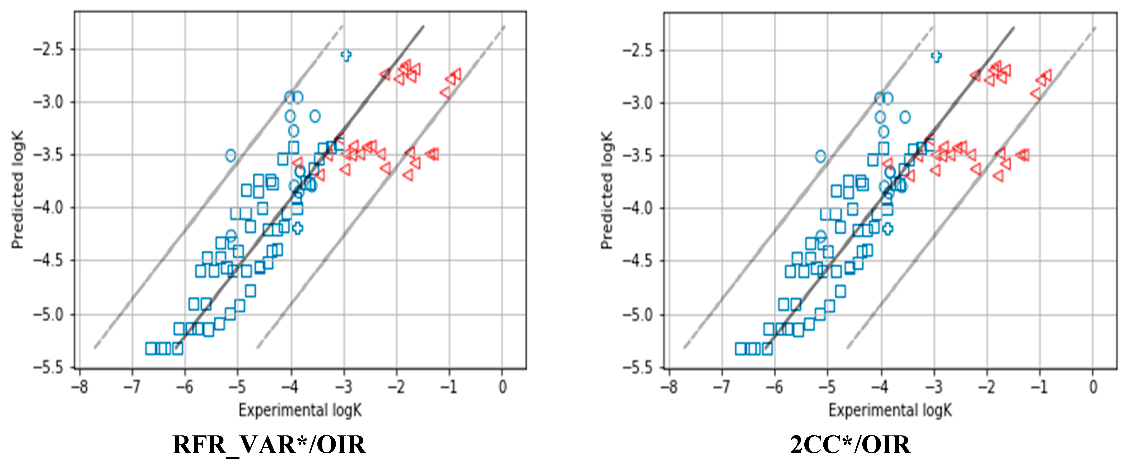
- OIR (Out and in RMSE)—the difference between RMSE of property prediction for reactions outside AD (denoted as RMSEOUT) and within AD (denoted as RMSEIN). The metric was first proposed by Sahigata et al. [25]. Negative values indicate that the reactions detected as X-outliers (outside AD) are predicted better than X-inliers (within AD), thus highlighting some possible drawbacks in the definition of interpolation space. Its positive values indicate the improvement in the property prediction within AD. If no reactions are left inside or outside AD, then OIR is considered equal to 0;
- (iii)
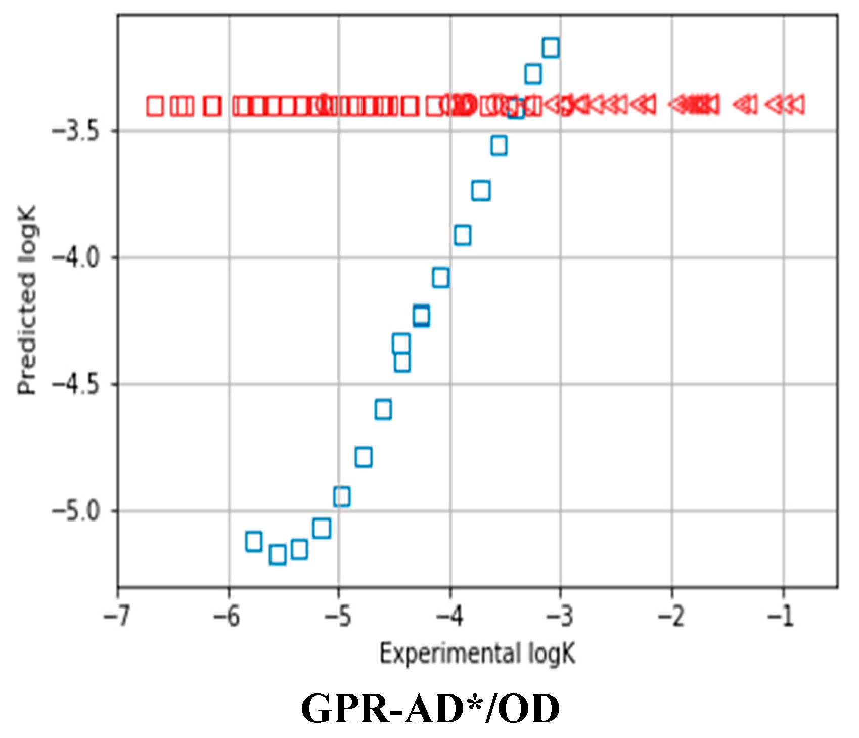
- The Outliers Criterion metric shows how well AD definition detects Y-outliers. First, property prediction errors are estimated in cross-validation for all reactions in a dataset. The reactions for which the absolute prediction error is higher than 3× RMSE are identified as Y-outliers, while the rest are considered as Y-inliers. Y-outliers (poorly predicted) that are predicted by AD definition as X-outliers (outside AD) are called true outliers (TO), while Y-inliers predicted by AD definition as X-inliers (within AD) are called true inliers (TI). False outliers (FO) are Y-inliers that are wrongly predicted by the AD definition as X-outliers, while false inliers (FI) are Y-outliers that are wrongly predicted by the AD definition as X-inliers. Then, the quality of outliers/inliers determination can be assessed using an analogue of the balanced accuracy and denoted as OD (Outliers Detection). OD = . In the “Perfect AD model”, the value of this parameter approaches the maximum possible value of 1;
- (iv)
- Area Under the ROC Curve (AUC_AD). This metric shows how well an AD definition can rank predictions made by the corresponding QRPR model from most reliable to least reliable. Reactions that are considered by AD definition as X-inliers (within AD) are considered as the positive class, while X-outliers are considered as the negative class. The absolute error of property prediction made by the corresponding QRPR model for a given reaction is used as a threshold for ROC curve construction. Thus, if the Area Under Curve (AUC) is large (close to 1), X-outliers are at the top of the list, sorted in descending order according to the error of prediction.
2.3. Model Building and Validation
2.4. Data Sets and Descriptors
3. Results and Discussion
3.1. Detection of a Reaction Type Missing in the Training Set
3.2. Coverage
3.3. Detection of Y-outliers
3.4. Enhancement of Prediction Quality
3.5. Ranking Different AD Definition Methods
3.6. Validating AD Definition Models on External Test Set
4. Conclusions
Supplementary Materials
Author Contributions
Funding
Conflicts of Interest
Abbreviations
| AD | Applicability Domain |
| QSAR/QSPR | Quantitative Structure–Activity/Property Relationship |
| OECD | Organization of Economic Co-operation and Development |
| QRPR model | Quantitative Reaction–Property Relationships model |
| ML-dependent AD | Applicability domain definition approaches that are tied to the machine learning method. It means that the determination of whether an object belongs to the model’s applicability domain and the prediction of property value for a given object is made by the machine-learning approach. |
| Universal AD | Applicability domain definition approaches that are not tied to the machine learning method. In this case, predicted property is given by Random Forest Regressor and the object’s belonging to the model’s applicability domain is determined in another way. |
| Leverage | Universal AD definition approach which based on the distance from the test sample objects to the centre of the training set distribution. |
| Lev_cv | Modification of Leverage approach. Leverage does not have internal hyperparameters, Lev_cv has one—the optimal threshold that needs to be adjusted. |
| Z-1NN | AD is defined on the basis of distance from a test set object to the most similar training set object(s). One nearest neighbour is considered. |
| Z-1NN_cv | Modification of Z-1NN_cv approach. Z-1NN doesn’t have internal hyperparameters, Z-1NN_cv has one—the optimal threshold that needs to be adjusted. |
| 1-SVM | One-Class Support Vector Machine |
| 2CC | Two-Class Classification method |
| RFClf | Random Forest Classifier |
| BB | Bounding Box |
| FC | Fragment Control |
| RTC_cv | Reaction Type Control. It needs to add «cv» since it is necessary to select the hyperparameter of the method |
| RTC* | Reaction Type Control with the first neighborhood |
| GPR | Gaussian Process Regression |
| RF | Random Forest Regressor |
| GPR-model | If structure-reactivity modelling is performed using Gaussian Process Regression |
| GPR-AD | The variance in prediction by Gaussian Process as AD measure |
| RFR_VAR | The variance in the ensemble of predictions as AD measure |
| Weak consensus | If most methods suggest that the reaction falls in AD, then it is predicted as belonging to AD |
| Strict consensus | The reaction belongs to AD if all the methods suggest that it falls in AD |
| OZ | “optimistic zero model” |
| PZ | “pessimistic zero model” |
| “Perfect AD model” | Exactly predicts inliers (reactions with prediction error less than 3xRMSE on cross-validation) and outliers (the rest). |
| RMSE | Root-mean-square error |
| R2 | Coefficient of determination |
| ∆R2_AD | It is the difference between the coefficient of determination for property prediction (R2) for objects within AD and corresponding value for all datapoints. |
| OIR | It is the difference between prediction RMSE for objects outside AD (denoted as RMSEOUT) and within AD (denoted as RMSEIN). |
| OD | Outliers Detection |
| AUC_AD | Area Under the ROC Curve as ranking criterion for AD detection |
| CV | Cross-validation |
| SN2 | Bimolecular nucleophilic substitution |
| DA | Diels–Alder reactions |
| E2 | Bimolecular elimination |
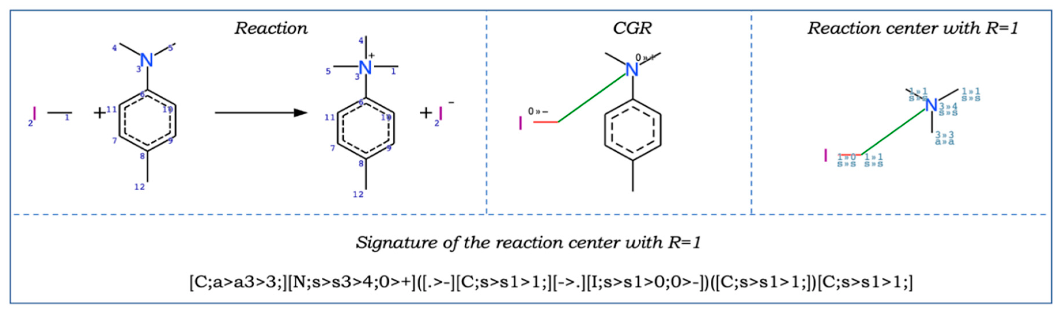
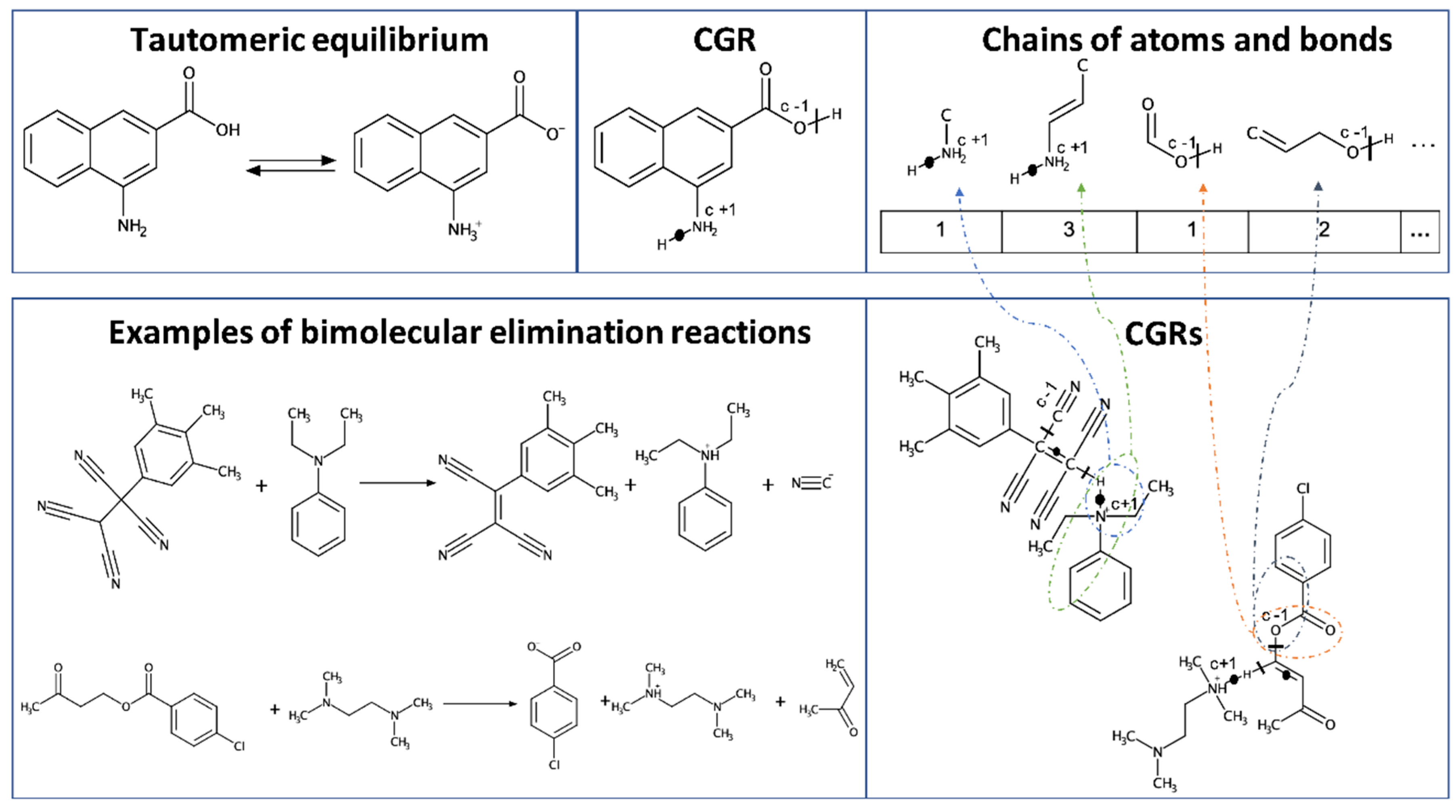
| CGR | Condensed Graph of Reaction |
References
- Cherkasov, A.; Muratov, E.N.; Fourches, D.; Varnek, A.; Baskin, I.I.; Cronin, M.; Dearden, J.; Gramatica, P.; Martin, Y.C.; Todeschini, R.; et al. QSAR modeling: Where have you been? Where are you going to? J. Med. Chem. 2014, 57, 4977–5010. [Google Scholar] [CrossRef]
- Roy, K.; Kar, S.; Das, R.N. Understanding the Basics of QSAR for Applications in Pharmaceutical Sciences and Risk Assessment; Academic Press: Boston, MA, USA, 2015. [Google Scholar]
- Jaworska, J.; Nikolova-Jeliazkova, N.; Aldenberg, T. QSAR applicability domain estimation by projection of the training set descriptor space: A review. Altern. Lab. Anim. 2005, 33, 445–459. [Google Scholar] [CrossRef]
- Netzeva, T.; Worth, A.; Aldenberg, T.; Benigni, R.; Cronin, M.; Gramatica, P.; Jaworska, J.; Kahn, S.; Klopman, G.; Marchant, C.; et al. Current status of methods for defining the applicability domain of (Quantitative) Structure–Activity Relationships. Altern. Lab. Anim. 2005, 33, 155–173. [Google Scholar] [CrossRef]
- Tetko, I.V.; Sushko, I.; Pandey, A.K.; Zhu, H.; Tropsha, A.; Papa, E.; Oberg, T.; Todeschini, R.; Fourches, D.; Varnek, A. Critical assessment of QSAR models of environmental toxicity against Tetrahymena pyriformis: Focusing on applicability domain and overfitting by variable selection. J. Chem. Inf. Model. 2008, 48, 1733–1746. [Google Scholar] [CrossRef]
- Sushko, I.; Novotarskyi, S.; Körner, R.; Pandey, A.K.; Cherkasov, A.; Li, J.; Gramatica, P.; Hansen, K.; Schroeter, T.; Müller, K.R.; et al. Applicability domains for classification problems: Benchmarking of distance to models for Ames mutagenicity set. J. Chem. Inf. Model. 2010, 50, 2094–2111. [Google Scholar] [CrossRef]
- OECD (2014) Guidance Document on the Validation of (Quantitative) Structure-Activity Relationship [(Q)SAR] Models; OECD Publishing: Paris, France, 2007. [CrossRef]
- Gadaleta, D.; Mangiatordi, G.F.; Catto, M.; Carotti, A.; Nicolotti, O. Applicability Domain for QSAR Models: Where Theory Meets Reality. Int. J. Quant. Struct.-Prop. Relationsh. 2016, 1, 19. [Google Scholar] [CrossRef]
- Mathea, M.; Klingspohn, W.; Baumann, K. Chemoinformatic classification methods and their applicability domain. Mol. Inf. 2016, 35, 160–180. [Google Scholar] [CrossRef]
- Klingspohn, W.; Mathea, M.; Laak, A.; Heinrich, N.; Baumann, K. Efficiency of different measures for defining the applicability domain of classification models. J. Cheminform. 2017, 9, 9–44. [Google Scholar] [CrossRef]
- Fechner, N.; Jahn, A.; Hinselmann, G.; Zell, A. Estimation of the applicability domain of kernel-based machine learning models for virtual screening. J. Cheminform. 2010, 2, 1–20. [Google Scholar] [CrossRef]
- Hanser, T.; Barber, C.; Marchaland, J.F.; Werner, S. Applicability domain: Towards a more formal definition. SAR QSAR Environ. Res. 2016, 27, 893–909. [Google Scholar] [CrossRef]
- Baskin, I.I.; Madzhidov, T.I.; Antipin, I.S.; Varnek, A.A. Artificial Intelligence in Synthetic Chemistry: Achievements and Prospects. Russ. Chem. Rev. 2017, 86, 1127–1156. [Google Scholar] [CrossRef]
- Coley, C.W.; Green, W.H.; Jensen, K.F. Machine Learning in Computer-Aided Synthesis Planning. Acc. Chem. Res. 2018, 51, 1281–1289. [Google Scholar] [CrossRef]
- Engkvist, O.; Norrby, P.O.; Selmi, N.; Lam, Y.; Peng, Z.; Sherer, E.C.; Amberg, W.; Erhard, T.; Smyth, L.A. Computational Prediction of Chemical Reactions: Current Status and Outlook. Drug Discov. Today 2018, 23, 1203–1218. [Google Scholar] [CrossRef]
- Gimadiev, T.; Madzhidov, T.; Tetko, I.; Nugmanov, R.; Casciuc, I.; Klimchuk, O.; Bodrov, A.; Polishchuk, P.; Antipin, I.; Varnek, A. Bimolecular Nucleophilic Substitution Reactions: Predictive Models for Rate Constants and Molecular Reaction Pairs Analysis. J. Mol. Inf. 2018, 38, 1800104. [Google Scholar] [CrossRef]
- Kravtsov, A.A.; Karpov, P.V.; Baskin, I.I.; Palyullin, V.A.; Zefirov, N.S. Prediction of rate constants of SN2 reactions by the Multicomponent QSPR method. Dokl. Chem. 2011, 440, 299–301. [Google Scholar] [CrossRef]
- Nugmanov, R.I.; Madzhidov, T.I.; Haliullina, G.R.; Baskin, I.I.; Antipin, I.S.; Varnek, A. Development of “structure-reactivity” models for nucleophilic substitution reactions with participation of azides. J. Struct. Chem. 2014, 55, 1026–1032. [Google Scholar] [CrossRef]
- Kravtsov, A.A.; Karpov, P.V.; Baskin, I.I.; Palyullin, V.A.; Zefirov, N.S. Prediction of the preferable mechanism of nucleophilic substitution at saturated carbon atom and prognosis of SN1 rate constants by means of QSPR. Dokl. Chem. 2011, 441, 314–317. [Google Scholar] [CrossRef]
- Polishchuk, P.; Madzhidov, T.I.; Gimadiev, T.R.; Bodrov, A.V.; Nugmanov, R.I.; Varnek, A. Structure-reactivity modeling using mixture-based representation of chemical reactions. J. Comput.-Aided Mol Des. 2017, 31, 829–839. [Google Scholar] [CrossRef]
- Madzhidov, T.I.; Bodrov, A.V.; Gimadiev, T.R.; Nugmanov, R.I.; Antipin, I.S.; Varnek, A. Structure–reactivity relationship in bimolecular elimination reactions based on the condensed graph of a reaction. J. Struct. Chem. 2015, 56, 1227–1234. [Google Scholar] [CrossRef]
- Madzhidov, T.I.; Gimadiev, T.R.; Malakhova, D.A.; Nugmanov, R.I.; Baskin, I.I.; Antipin, I.S.; Varnek, A. Structure-Reactivity modelling for Diels-alder reactions based on the condensed REACTION graph approach. J. Struct. Chem. 2017, 58, 685–691. [Google Scholar] [CrossRef]
- Gimadiev, T.; Madzhidov, T.; Nugmanov, R.; Baskin, I.; Antipin, I.; Varnek, A. Assessment of tautomer distribution using the condensed reaction graph approach. J. Comput.-Aided Mol. Des. 2018, 32, 401–414. [Google Scholar] [CrossRef] [PubMed]
- Gao, H.; Struble, T.J.; Coley, C.W.; Wang, Y.; Green, W.H.; Jensen, K.F. Using Machine Learning to Predict Suitable Conditions for Organic Reactions. ACS Cent. Sci. 2018, 4, 1465–1476. [Google Scholar] [CrossRef] [PubMed]
- Sahigara, F.; Mansouri, K.; Ballabio, D.; Mauri, A.; Consonni, V.; Todeschini, R. Comparison of Different Approaches to Define the Applicability Domain of QSAR Models. Molecules 2012, 17, 4791–4810. [Google Scholar] [CrossRef] [PubMed]
- Baskin, I.; Kireeva, N.; Varnek, A. The One-Class Classification Approach to Data Description and to Models Applicability Domain. J. Mol. Inf. 2010, 29, 581–587. [Google Scholar] [CrossRef]
- Scikit-Learn User Guide. Available online: https://scikit-learn.org/stable/_downloads/scikit-learn-docs.pdf (accessed on 2 August 2020).
- Varnek, A.; Fourches, D.; Hoonakker, F.; Solov’ev, V.P. Substructural fragments: A universal language to encode reactions, molecular and supramolecular structures. J. Comput. Aided Mol. Des. 2005, 19, 693–703. [Google Scholar] [CrossRef]
- Hoonakker, F.; Lachiche, N.; Varnek, A. Condensed Graph of Reaction: Considering a chemical reaction as one single pseudo molecule. Int. J. Artif. Intell. Tools 2011, 20, 253–270. Available online: https://dtai.cs.kuleuven.be/events/ilp-mlg-srl/papers/ILP09-5.pdf (accessed on 2 August 2020). [CrossRef]
- Varnek, A. ISIDA—Platform for Virtual Screening Based on Fragment and Pharmacophoric Descriptors. Curr. Comput.-Aided Drug Des. 2008, 4, 191–198. [Google Scholar] [CrossRef]
- Nugmanov, R.I.; Mukhametgaleev, R.N.; Akhmetshin, T.; Gimadiev, T.R.; Afonina, V.A.; Madzhidov, T.I.; Varnek, A. CGRtools: Python Library for Molecule, Reaction, and Condensed Graph of Reaction Processing. J. Chem. Inf. Model. 2019, 59, 2516–2521. [Google Scholar] [CrossRef]
- Rasmussen, C.E.; Williams, C.K.I. Gaussian Processes for Machine Learning; MIT Press: Cambridge, MA, USA, 2006; ISBN 026218253X. Available online: http://www.gaussianprocess.org/gpml/chapters/RW.pdf (accessed on 2 August 2020).
- Varma, S.; Simon, R. Bias in error estimation when using cross-validation for model selection. BMC Bioinform. 2006, 7, 91. [Google Scholar] [CrossRef]
- Catalán, J.; López, V.; Pérez, P. Progress towards a generalized solvent polarity scale: The solvatochromism of 2-(dimethylamino)-7-nitrofluorene and its homomorph 2-fluoro-7-nitrofluorene. Liebigs Ann. 1995, 241–252. [Google Scholar] [CrossRef]
- Catalaán, J.; Díaz, C.A. generalized solvent acidity scale: The solvatochromism of o-tert-butylstilbazolium betaine dye and its homomorph o,o′-di-tert-butylstilbazolium betaine dye. Liebigs Ann. 1997, 1941–1949. [Google Scholar] [CrossRef]
- Kamlet, M.J.; Taft, R.W. The solvatochromic comparison method. I. The beta scale of solvent hydrogen-bond acceptor (HBA) basicities. J. Am. Chem. Soc. 1976, 98, 377–383. [Google Scholar] [CrossRef]
- Taft, R.W.; Kamlet, M.J. The solvatochromic comparison method. 2. The alpha scale of solvent hydrogen-bond donor (HBD) acidities. J. Am. Chem. Soc. 1976, 98, 2886–2894. [Google Scholar] [CrossRef]
- Kamlet, M.J.; Abboud, J.L.; Taft, R.W. The solvatochromic comparison method. 6. The pi * scale of solvent polarities. J. Am. Chem. Soc. 1977, 99, 6027–6038. [Google Scholar] [CrossRef]
- Madzhidov, T.I.; Polishchuk, P.G.; Nugmanov, R.I.; Bodrov, A.V.; Lin, A.I.; Baskin, I.I.; Varnek, A.A.; Antipin, I.S. Structure-reactivity relationships in terms of the condensed graphs of reactions. Russ. J. Org. Chem. 2014, 50, 459–463. [Google Scholar] [CrossRef]
- Horvath, D.; Marcou, G.; Varnek, A. A unified approach to the applicability domain problem of QSAR models. J. Cheminform. 2010, 2, O6. [Google Scholar] [CrossRef]


| Universal AD Definition Approaches | Machine Learning (ML)-Dependent AD Definition Approaches | |
|---|---|---|
| Without Hyperparameters | With Hyperparameters | With Hyperparameters |
| BB | RTC_cv | GPR-AD |
| FC | 2CC_cv | RFR_VAR |
| Z-1NN | 1-SVM | |
| Leverage | Z-1NN_cv | |
| Leverage_cv | ||
| Regression Method | DA | SN2 | Tautomerization | E2 | |
|---|---|---|---|---|---|
| RFR | R2 | 0.854 | 0.804 | 0.682 | 0.708 |
| RMSE | 0.734 | 0.516 | 0.914 | 0.799 | |
| GPR | R2 | 0.807 | 0.763 | 0.492 | 0.648 |
| RMSE | 0.845 | 0.568 | 1.156 | 0.876 |
| № | AD Definition Method | Coverage | OIR | ∆R2_AD | OD | ||||||||||||
|---|---|---|---|---|---|---|---|---|---|---|---|---|---|---|---|---|---|
| SN2 | DA | E2 | Tautomerization | SN2 | DA | E2 | Tautomerization | SN2 | DA | E2 | Tautomerization | SN2 | DA | E2 | Tautomerization | ||
| ML-Dependent AD Definition Methods | |||||||||||||||||
| 1 | RFR_VAR*/OIR | 0.98 | 0.94 | 0.93 | 0.95 | 0.66 | 1.38 | 0.71 | 1.63 | 0.01 | 0.05 | 0.04 | −0.05 | 0.56 | 0.73 | 0.68 | 0.73 |
| 2 | GPR-AD*/OIR | 0.97 | 0.94 | 0.92 | 0.96 | 0.70 | 0.67 | 0.41 | 1.73 | 0.03 | 0.05 | 0.05 | 0.01 | 0.63 | 0.73 | 0.75 | 0.72 |
| 3 | RFR_VAR*/OD | 0.79 | 0.83 | 0.81 | 0.90 | 0.51 | 1.22 | 0.57 | 1.74 | 0.07 | 0.10 | 0.10 | −0.11 | 0.80 | 0.86 | 0.76 | 0.91 |
| 4 | GPR-AD*/OD | 0.89 | 0.78 | 0.81 | 0.93 | 0.78 | 0.38 | 0.07 | 1.60 | 0.09 | 0.08 | 0.08 | −0.03 | 0.80 | 0.79 | 0.84 | 0.82 |
| Universal AD definition methods with hyperparameters | |||||||||||||||||
| 5 | 2CC*/OIR | 0.98 | 0.94 | 0.92 | 0.94 | 0.67 | 1.62 | 0.46 | 1.83 | 0.02 | 0.06 | 0.02 | −0.10 | 0.59 | 0.77 | 0.63 | 0.76 |
| 6 | Lev_cv*/OIR | 0.98 | 0.94 | 0.75 | 0.96 | 0.61 | 1.39 | 0.15 | 1.59 | 0.01 | 0.05 | 0.02 | −0.05 | 0.55 | 0.71 | 0.59 | 0.69 |
| 7 | Z-1NN_cv*/OIR | 0.98 | 0.94 | 0.93 | 0.95 | 0.60 | 1.39 | 0.50 | 1.53 | 0.01 | 0.05 | 0.03 | −0.09 | 0.55 | 0.71 | 0.63 | 0.69 |
| 8 | 1-SVM*/OIR | 0.98 | 0.94 | 0.86 | 0.86 | 0.57 | 1.34 | 0.35 | 0.79 | 0.01 | 0.05 | 0.03 | −0.13 | 0.56 | 0.71 | 0.67 | 0.68 |
| 9 | 2CC*/OD | 0.84 | 0.82 | 0.80 | 0.89 | 0.59 | 1.12 | 0.44 | 1.64 | 0.07 | 0.09 | 0.09 | −0.12 | 0.82 | 0.83 | 0.74 | 0.87 |
| 10 | Lev_cv*/OD | 0.83 | 0.72 | 0.85 | 0.82 | 0.28 | 0.59 | 0.42 | 1.13 | 0.03 | 0.07 | 0.07 | −0.15 | 0.61 | 0.73 | 0.74 | 0.83 |
| 11 | Z-1NN_cv*/OD | 0.79 | 0.73 | 0.81 | 0.74 | 0.35 | 0.69 | 0.40 | 0.86 | 0.05 | 0.08 | 0.08 | −0.08 | 0.70 | 0.75 | 0.70 | 0.83 |
| 12 | 1-SVM*/OD | 0.49 | 0.29 | 0.68 | 0.66 | 0.22 | 0.37 | 0.28 | 0.42 | 0.07 | 0.07 | 0.07 | −0.21 | 0.69 | 0.62 | 0.72 | 0.67 |
| Universal AD definition methods without hyperparameters | |||||||||||||||||
| 13 | RTC1 | 0.98 | 0.94 | 0.93 | 0.96 | 0.61 | 1.39 | 0.51 | 1.59 | 0.01 | 0.05 | 0.03 | −0.05 | 0.55 | 0.71 | 0.63 | 0.69 |
| 14 | BB* | 0.98 | 0.94 | 0.93 | 0.94 | 0.58 | 1.34 | 0.50 | 1.30 | 0.01 | 0.05 | 0.03 | −0.05 | 0.56 | 0.71 | 0.63 | 0.68 |
| 15 | Leverage* | 0.95 | 0.93 | 0.91 | 0.92 | 0.45 | 1.29 | 0.55 | 1.19 | 0.02 | 0.05 | 0.04 | −0.19 | 0.60 | 0.72 | 0.67 | 0.71 |
| 16 | Z-1NN* | 0.95 | 0.91 | 0.90 | 0.92 | 0.44 | 1.09 | 0.64 | 1.16 | 0.02 | 0.05 | 0.06 | −0.12 | 0.60 | 0.74 | 0.71 | 0.71 |
| “Zero models” | |||||||||||||||||
| 17 | OZ | 1.00 | 1.00 | 1.00 | 1.00 | 0 | 0 | 0 | 0 | 0.00 | 0.00 | 0.00 | 0.00 | 0.50 | 0.50 | 0.50 | 0.50 |
| 18 | PZ | 0.00 | 0.00 | 0.00 | 0.00 | 0 | 0 | 0 | 0 | −0.81 | −0.85 | −0.71 | −0.70 | 0.50 | 0.50 | 0.50 | 0.50 |
| 19 | “Perfect AD model” | 0.98 | 0.98 | 0.99 | 0.98 | 1.75 | 3.75 | 2.71 | 4.08 | 0.06 | 0.08 | 0.05 | 0.06 | 1.00 | 1.00 | 1.00 | 1.00 |
| Data Set | ||||
|---|---|---|---|---|
| Rank | SN2 | Tautomerization | E2 | DA |
| 1 | “Perfect AD model” | “Perfect AD model” | “Perfect AD model” | “Perfect AD model” |
| 2 | GPR-AD*/OIR | RFR_VAR*/OIR | Z-1NN* | 2CC*/OIR |
| 3 | 2CC*/OD | GPR-AD*/OIR | RFR_VAR*/OIR | RFR_VAR*/OIR |
| 4 | GPR-AD*/OD | GPR-AD*/OD | GPR-AD*/OIR | RFR_VAR*/OD |
| 5 | RFR_VAR*/OIR | 2CC*/OIR | RFR_VAR*/OD | Lev_cv*/OIR |
| Best-Ranked Composite Ads | ||||
|---|---|---|---|---|
| № | AD Method | R2 | RMSE | Coverage |
| 1 | GPR-AD*/OIR | 0.96 | 0.17 | 17 |
| 2 | RFR_VAR*/OIR | 0.66 | 0.64 | 74 |
| 3 | 2CC*/OIR | 0.66 | 0.64 | 74 |
| 4 | GPR-AD*/OD | 0.96 | 0.17 | 17 |
| 5 | RFR_VAR*/OD | 0.80 | 0.39 | 34 |
| 6 | Z-1NN_cv*/OIR | 0.66 | 0.64 | 74 |
| 7 | 2CC*/OD | 0.67 | 0.53 | 25 |
| 8 | RTC1 | 0.66 | 0.64 | 74 |
| 9 | Z-1NN_cv*/OD | 0.94 | 0.22 | 17 |
| 10 | BB* | 0.66 | 0.64 | 73 |
| Without AD | 0.60 | 0.84 | 100 | |
© 2020 by the authors. Licensee MDPI, Basel, Switzerland. This article is an open access article distributed under the terms and conditions of the Creative Commons Attribution (CC BY) license (http://creativecommons.org/licenses/by/4.0/).
Share and Cite
Rakhimbekova, A.; Madzhidov, T.I.; Nugmanov, R.I.; Gimadiev, T.R.; Baskin, I.I.; Varnek, A. Comprehensive Analysis of Applicability Domains of QSPR Models for Chemical Reactions. Int. J. Mol. Sci. 2020, 21, 5542. https://doi.org/10.3390/ijms21155542
Rakhimbekova A, Madzhidov TI, Nugmanov RI, Gimadiev TR, Baskin II, Varnek A. Comprehensive Analysis of Applicability Domains of QSPR Models for Chemical Reactions. International Journal of Molecular Sciences. 2020; 21(15):5542. https://doi.org/10.3390/ijms21155542
Chicago/Turabian StyleRakhimbekova, Assima, Timur I. Madzhidov, Ramil I. Nugmanov, Timur R. Gimadiev, Igor I. Baskin, and Alexandre Varnek. 2020. "Comprehensive Analysis of Applicability Domains of QSPR Models for Chemical Reactions" International Journal of Molecular Sciences 21, no. 15: 5542. https://doi.org/10.3390/ijms21155542
APA StyleRakhimbekova, A., Madzhidov, T. I., Nugmanov, R. I., Gimadiev, T. R., Baskin, I. I., & Varnek, A. (2020). Comprehensive Analysis of Applicability Domains of QSPR Models for Chemical Reactions. International Journal of Molecular Sciences, 21(15), 5542. https://doi.org/10.3390/ijms21155542