Oritatami: A Computational Model for Molecular Co-Transcriptional Folding

Abstract
:1. Introduction
1.1. Main Contributions
1.2. Related Work
2. Model and Main Results
2.1. Model
2.1.1. Oritatami System
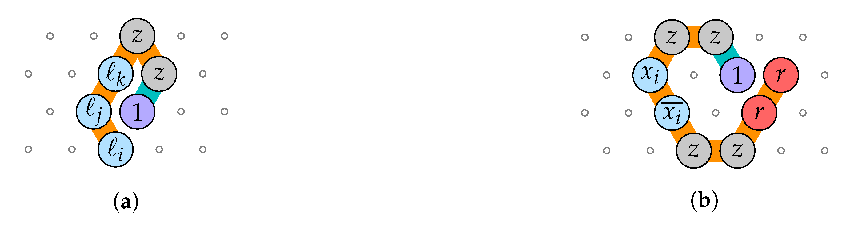
 , on the triangular lattice graph where if and only if . is composed of (1) a (possibly infinite) transcriptp, which is a sequence of beads, of a type chosen from a finite set B, (2) an attraction rule, which is a symmetric relation and (3) a parameter called the delay time. and a configuration c of a sequence w, we say that there is a bond between two adjacent positions and of c in if . The number of bonds in a configuration c of w, written , is the negation of the number of bonds within c: formally, wj}|.
2.1.2. Oritatami Dynamics
, and a seed configuration of a seed sequence s of length ℓ, a dynamics gives at each time step the set of favored nascent configurations of transcript p, as a function of the set of favored nascent configurations at the previous time step. Initially, the set of favored nascent configurations is , that is all the possible elongations of the seed configuration by beads. Then, the set of favored nascent configurations at step t is , that is the set of all elongations by beads of the seed configuration prolongated by the transcript according to dynamics .- The inertial dynamics
- was also called hasty dynamics in a preliminary version of this work [37]. It does not question previous choices but chooses the energy-minimal positions for the nascent beads among all elongations of the previously adopted partial configurations. It lets the already placed nascent beads where they are and abandons the extension of a configuration if no extension with the newly transcribed bead allows to reach a lowest energy configuration available for the nascent beads.Formally, given a set of currently favored nascent configurations, elongates each of them by one bead, and keeps the elongated configurations that have minimum energy among those who share the same prefix of length :
- The oblivious dynamics
- is oblivious in the sense that it consists of always choosing the best available positions for the nascent beads regardless of the previously preferred choices, as opposed to . Formally, takes a set of currently favored nascent configurations, removes the last positions from all of them, and selects the minimal energy configurations among all of their elongations by beads. Precisely:
is deterministic for dynamics and seed of sequence s if for all , the position of the i-th bead of p is uniquely determined at time i, i.e., if for all , .3. Folding a Binary Counter
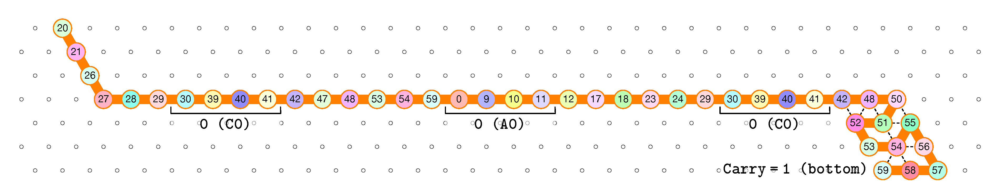
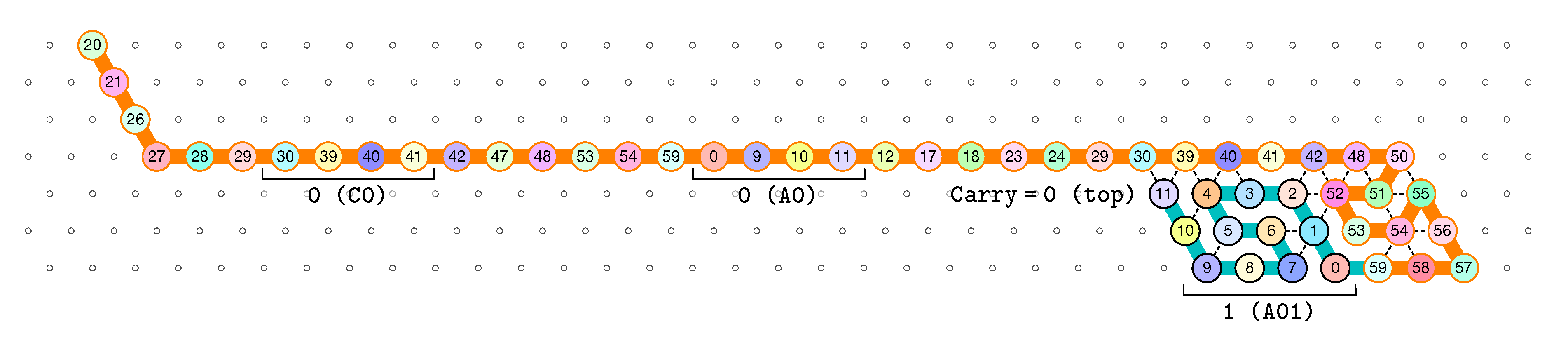
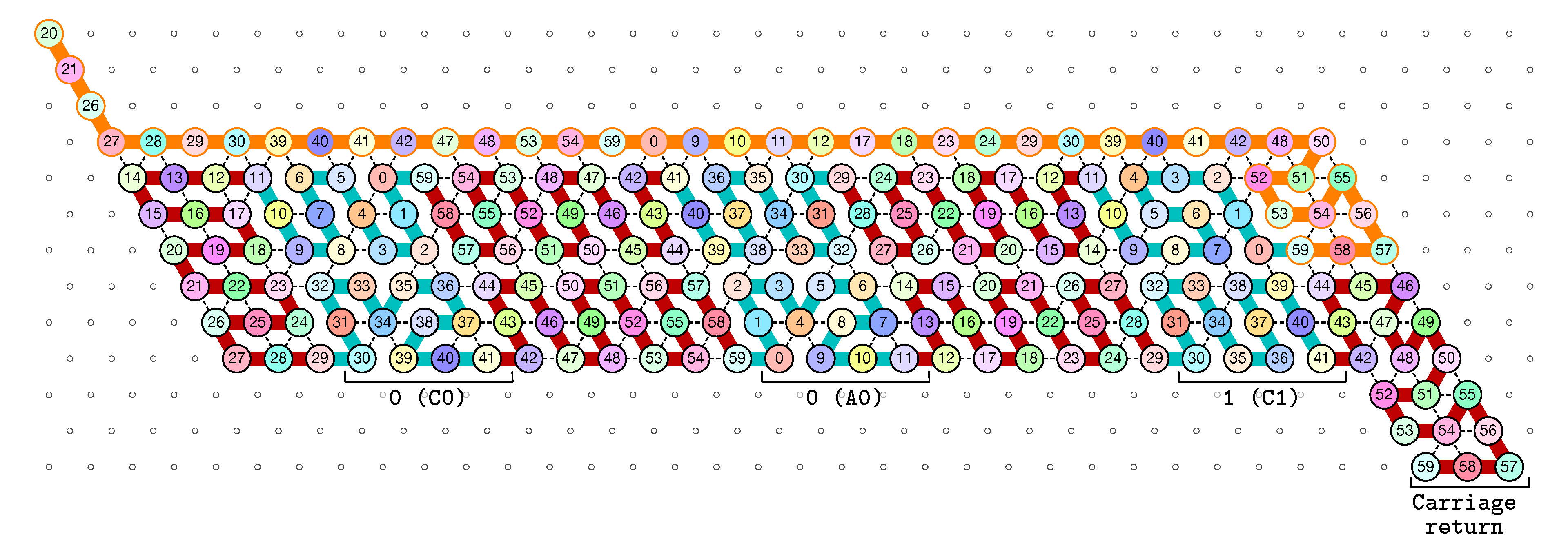
3.1. General Idea of The Construction
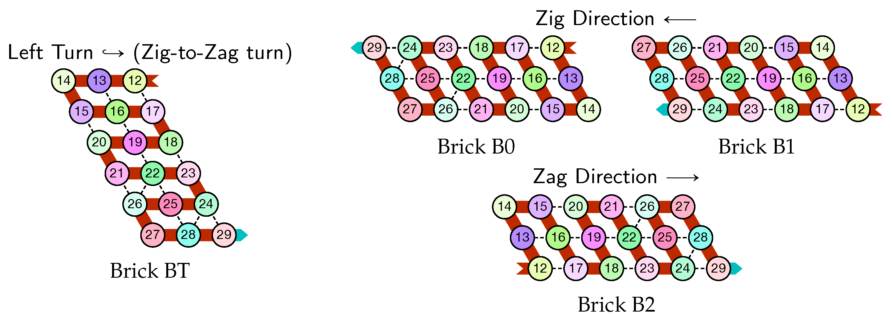
- Module A (beads 0–11, in blue in all figures): the First Half-Adder
- Module B (beads 12–29, in red in all figures): the Left-Turn module
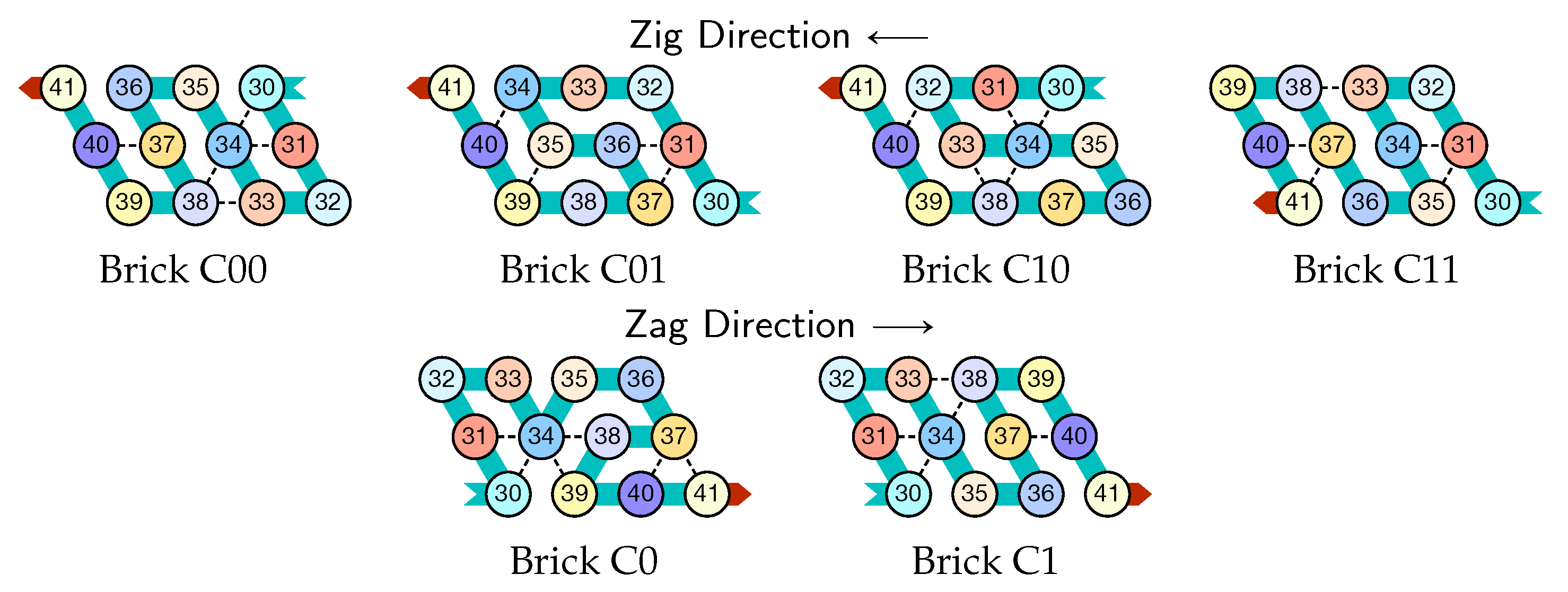
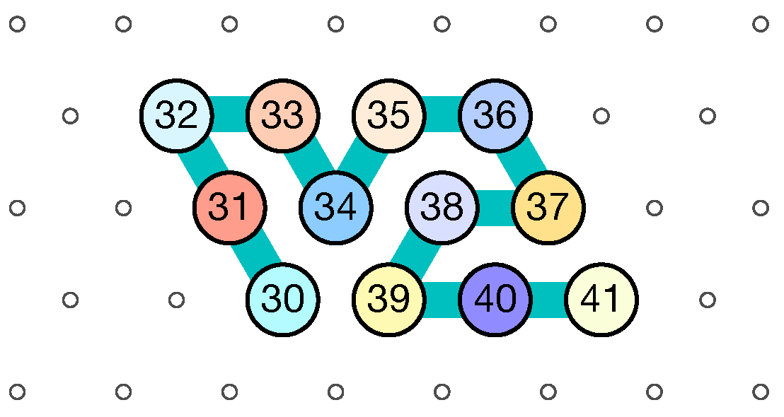
- Module C (beads 30–41, in blue in all figures): the Second Half-Adder
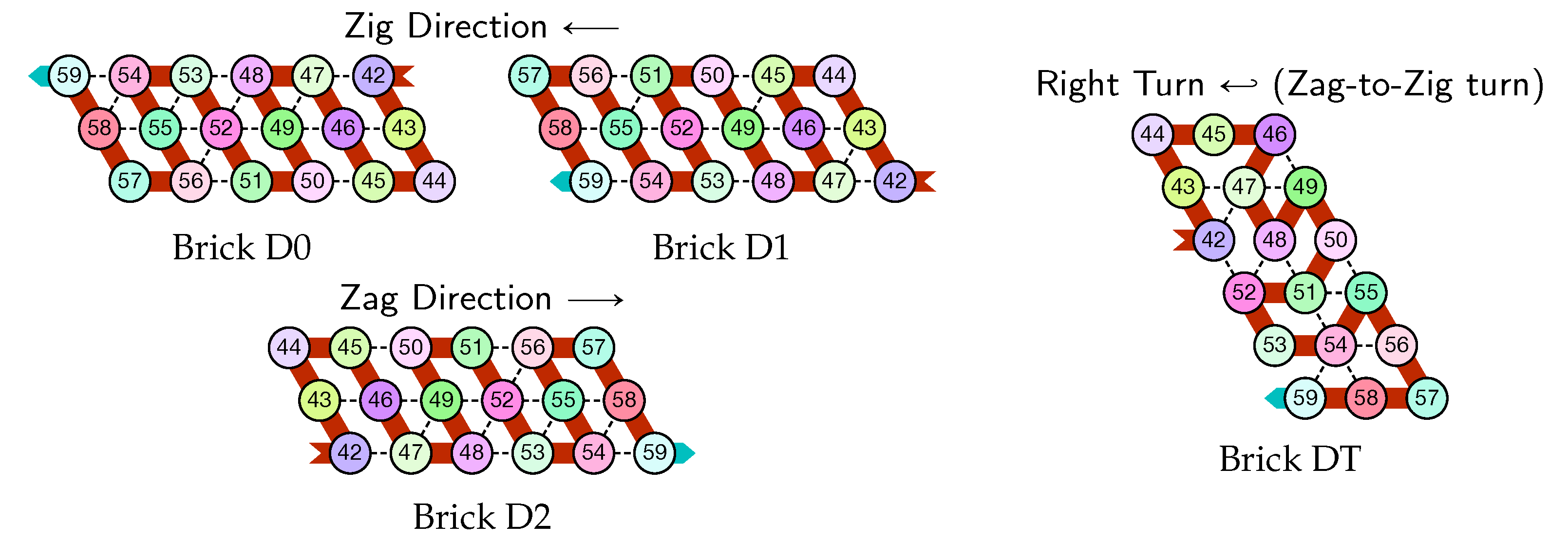
- Module D (beads 42–59, in red in all figures): the Right-Turn module
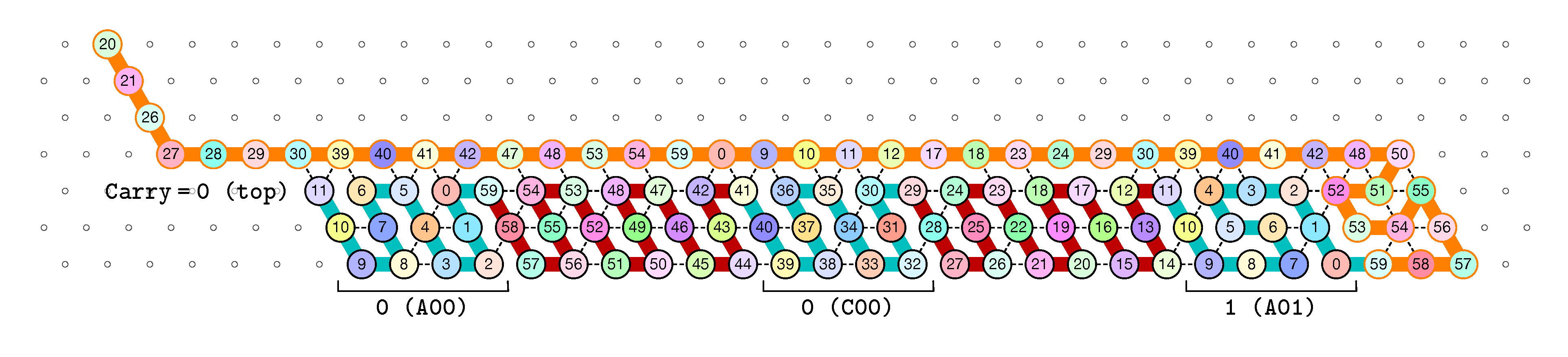
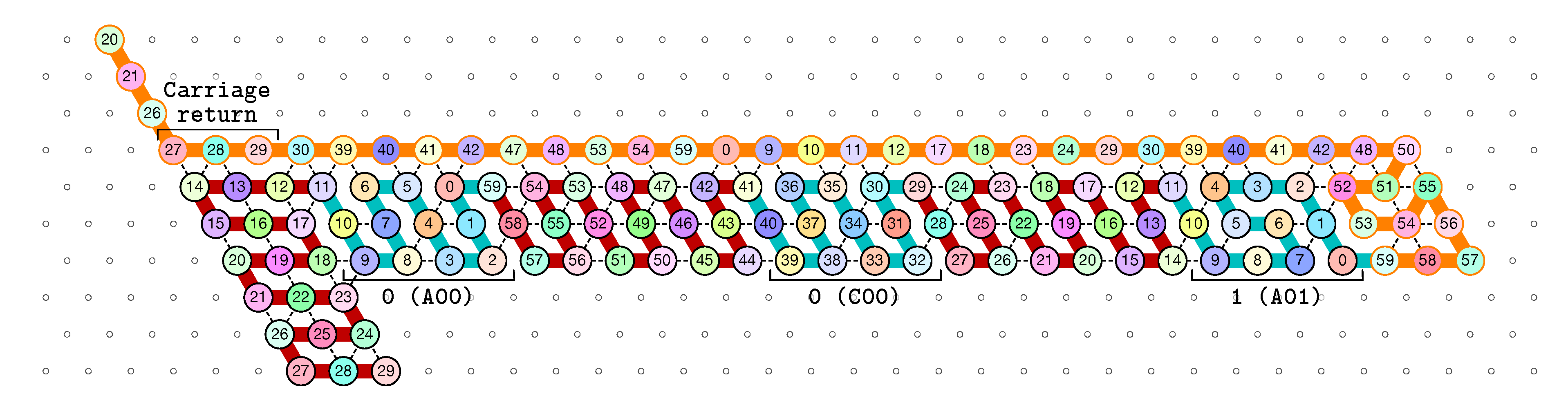
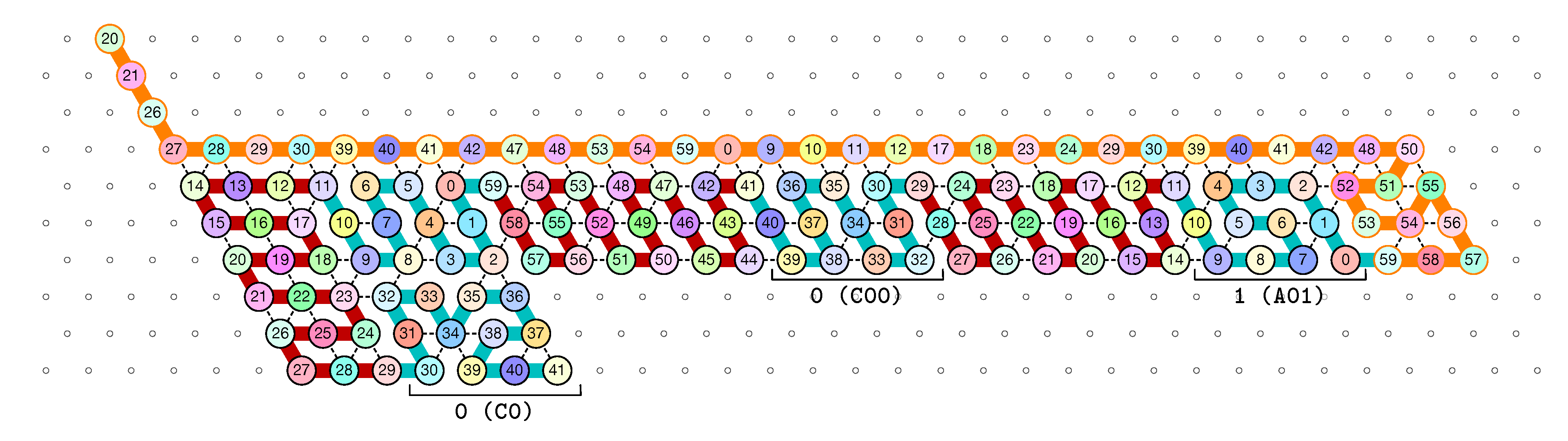
3.2. The First Two Passes of The Folding
- The first part , made of beads from Module B, encodes a sequence that will trigger the carriage return at the end of the next zig pass.
- The central part consists in k repetitions of the same sequence of 4 patterns, plus an extra repetition of the first pattern at the end (the central part consists thus in parts in total):
- -
- encoding a bit 0 using beads from Module C,
- -
- followed by encoding nothing but padding using beads from Module B,
- -
- followed by encoding a bit 0 using beads from Module A,
- -
- followed by encoding nothing but padding using beads from Module D.
Note the symmetry by a shift of 30 of the beads values in the patterns involving Modules A and C, and Modules B and D. - The last part , made of beads from Module D, encodes a sequence that will first initiate the next zig pass and later trigger the carriage return at the end of the next zag pass.
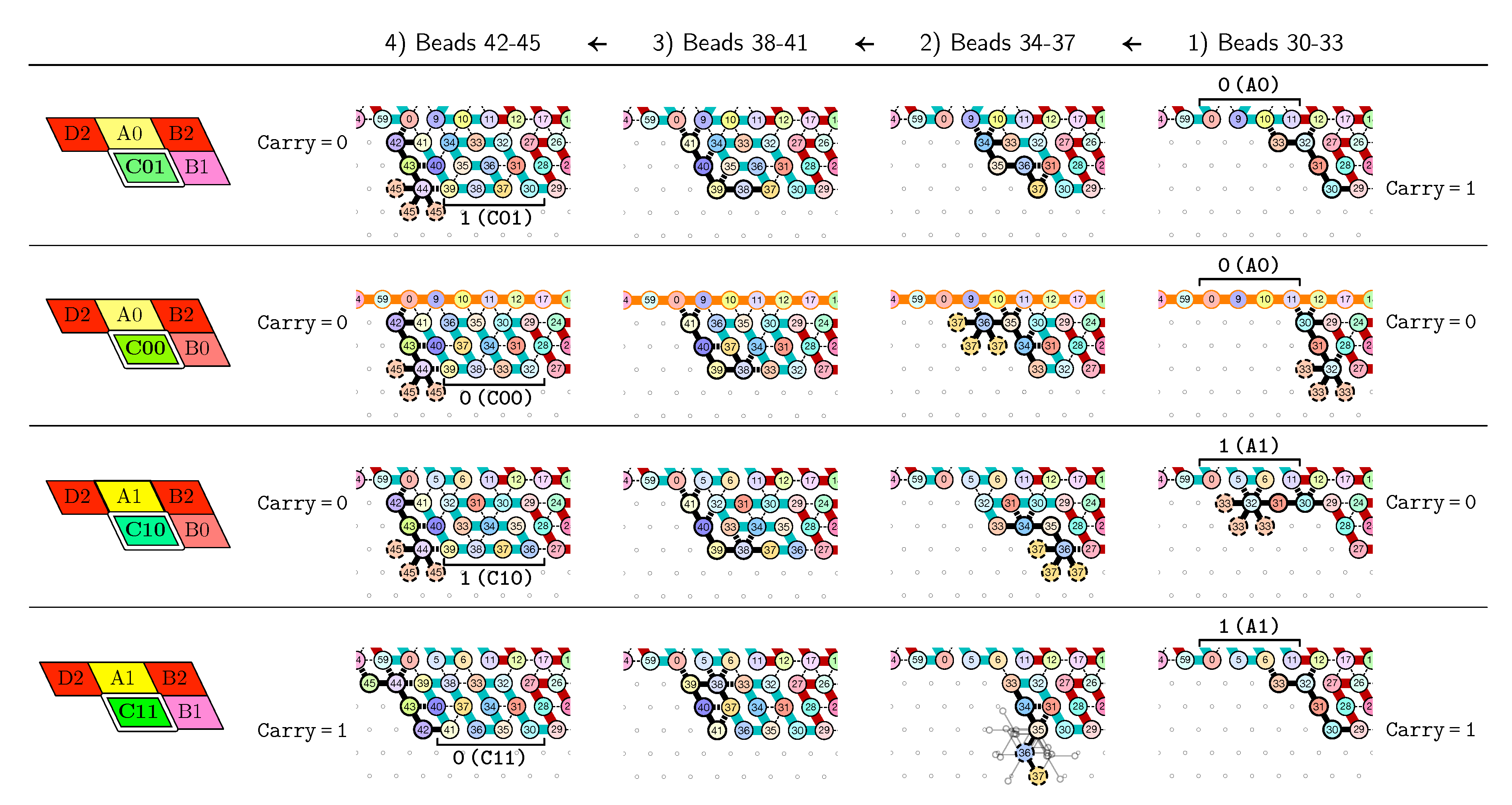
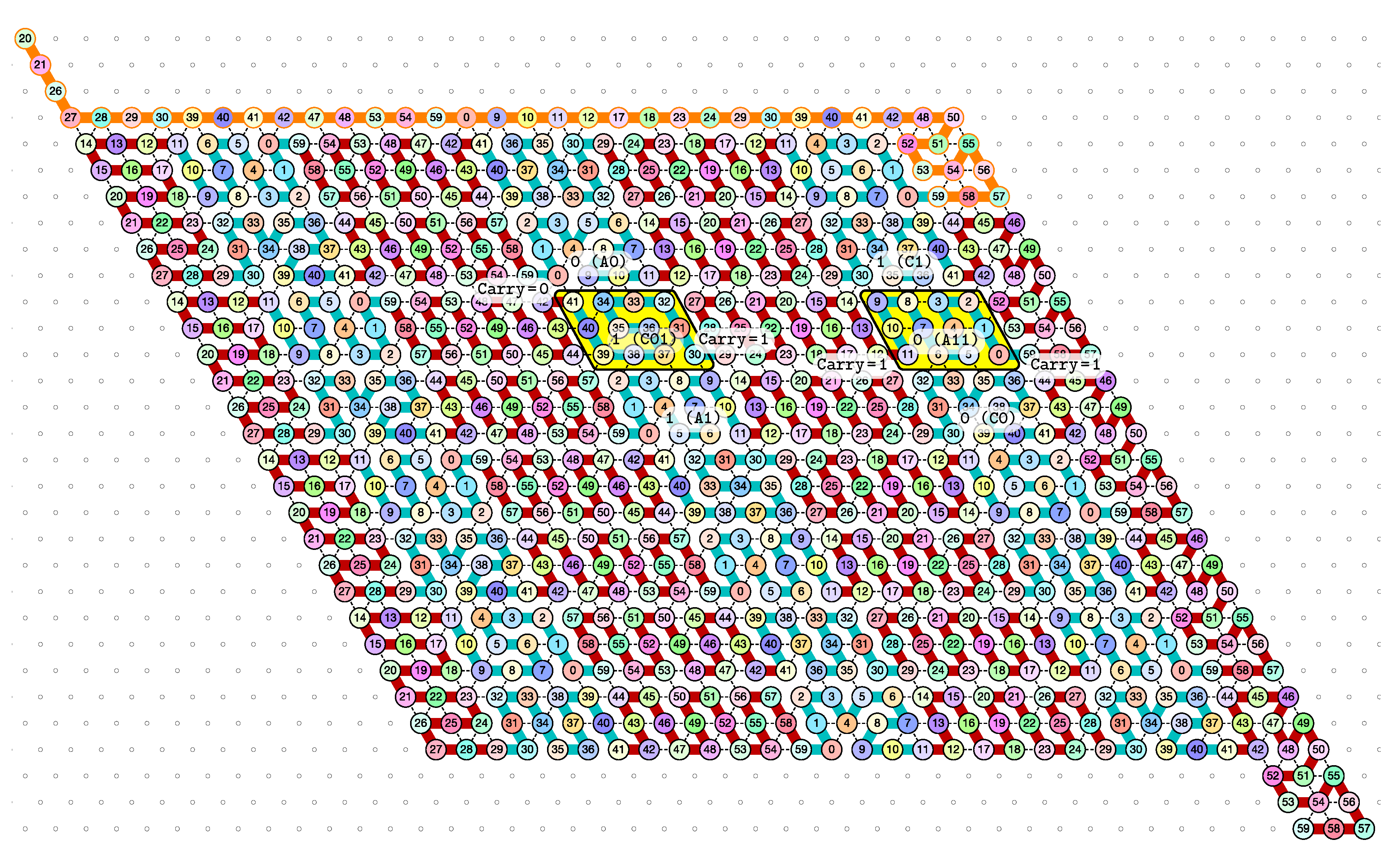
3.3. How Does Computation Take Place: Modules, Functions, States and Environment
- the current “state” of the molecule:
- here, the state is whether the carry is 0 or 1. As mentionned earlier this is encoded in the position of the molecule when the module starts to fold: it starts in the top row if the carry is 0; in the bottom row if the carry is 1.
- the local environment of the molecule:
- the environment, i.e., the beads already placed around the current area where the folding takes place, acts as the memory in the computation.
- Beads 30–33 (rightmost column in Figure 13):
- if the carry is 0 at start, then bead 30 is able to bind with beads 11 and 12 from the environment and depending on whether the input encodes a bit 0 or 1, bead 32 will be able to bind either to 28 or to 5 and 6 respectively. Whereas if the carry is 1, then bead 30 cannot reach the beads 11 and 12. Thus, these are beads 31 and 32 that will bind with beads 10 and 12 from the environment, giving to the molecule a completely different shape.
- Beads 34–37 with carry = 0 at start:
- as bead 34 is attracted by both beads 30 and 31, the molecule folds upon itself similarly but with a different rotation depending on whether it has read a 0 or a 1 in the environment above: vertically if it has read a 0, horizontally if it has read a 1. Bead 36 attracted by beads 9 and 27 fixes the end of the tip in place leaving bead 37 free to move for now.
- Beads 34–37 with carry = 1 at start:
- Bead 34 is attracted by beads 9 and 10 encoding a bit 0 above which allows beads 36 and 37 to bind with 31 as well, but prefers to bind with 31 together with 35 otherwise. This induces two different shapes: the beginning of a “wave” pattern (
![Ijms 20 02259 i002]() ) if the bit read above is 0; or the beginning of a “switchback” pattern (
) if the bit read above is 0; or the beginning of a “switchback” pattern ( ![Ijms 20 02259 i009]() ) if the bit read is 1.
) if the bit read is 1. - Beads 38–41, without carry propagation (carry = 0, or carry = 1 and bit read = 0):
- in these three cases the folding of the beads 38–41 starts from the same position. As the environment is different for each of them, we could design the rule so that this part of the module prefers to adopt the same shape, climing along the part already folded to the top row to start the next module with a carry .
- Beads 38-41, with carry propagation (carry = 1 and bit read = 1):
- because the switchback pattern is upside down in this case, bead 37 stays low and bead 38 can firmly attach to the top with beads 5, 6 and 33, and the tip of the module folds downwards as 40 and 41 are attracted by 37. This ensures that the folding of the module ends at the bottom row, propagating the carry to the next module.


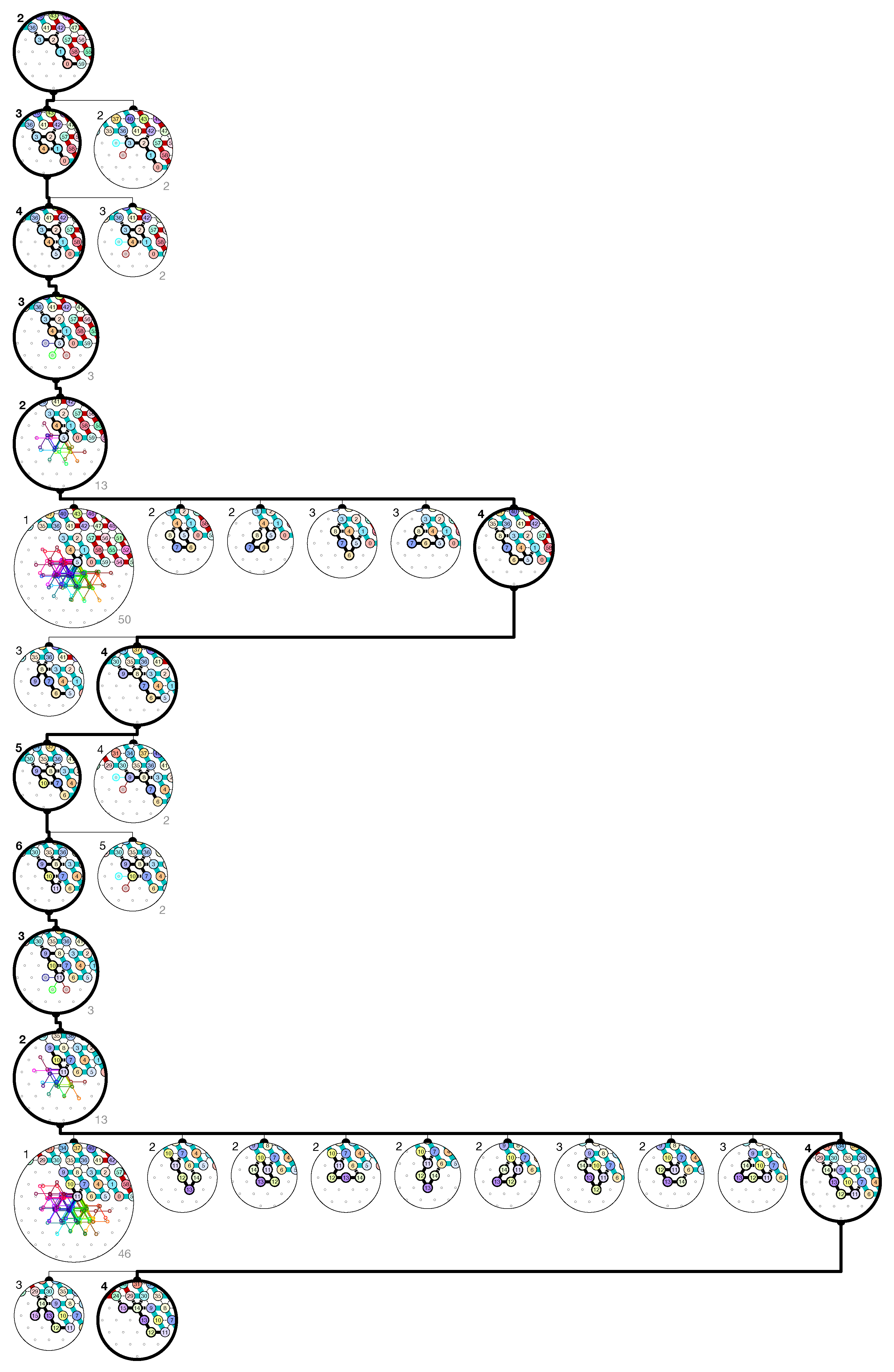
4. Proof of Correctness (Theorem 1)
4.1. Overview
- Module A (beads 0–11): the First Half-Adder
- Module B (beads 12–29): the Left-Turn module
- Module C (beads 30–41): the Second Half-Adder
- Module D (beads 42–59): the Right-Turn module
- A and C in the zig pass where are the bit read from the brick above (Ax or Cx) and the (input) carry from the preceding module (Bc or Dc);
- Ay and Cy in the zag pass where y is the bit written: namely if the brick above is A or C.
- B and D in the zig pass where is the carry output by the preceding brick C or A, namely ;
- and B2 and D2 in the zag pass.
4.2. Description of the Final Configuration (I.e., the Resulting Folding)
- Module A, First Half-Adder (beads 0–11):
![Ijms 20 02259 i003]()
- Module B, Left-Turn module (beads 12–29)
![Ijms 20 02259 i004]()
- Module C, Second Half-Adder (beads 30–41)
![Ijms 20 02259 i005]()
- Module D, Right-Turn module (beads 42–59)
![Ijms 20 02259 i006]()

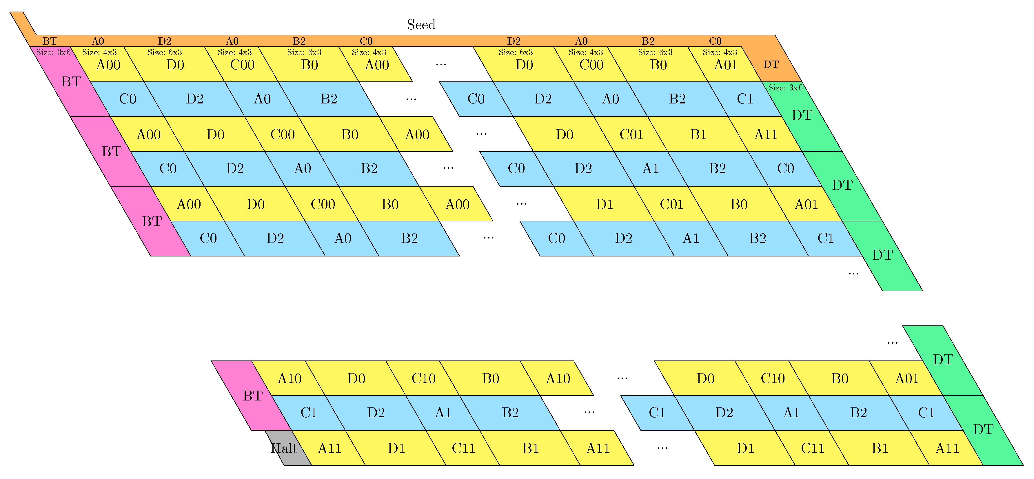
- The rightmost and leftmost columns have width 3:
- -
- The leftmost column consists in -regions all populated with the brick BT (Left Turn).
- -
- The rightmost column consists in -regions all populated with the brick DT (Right Turn).
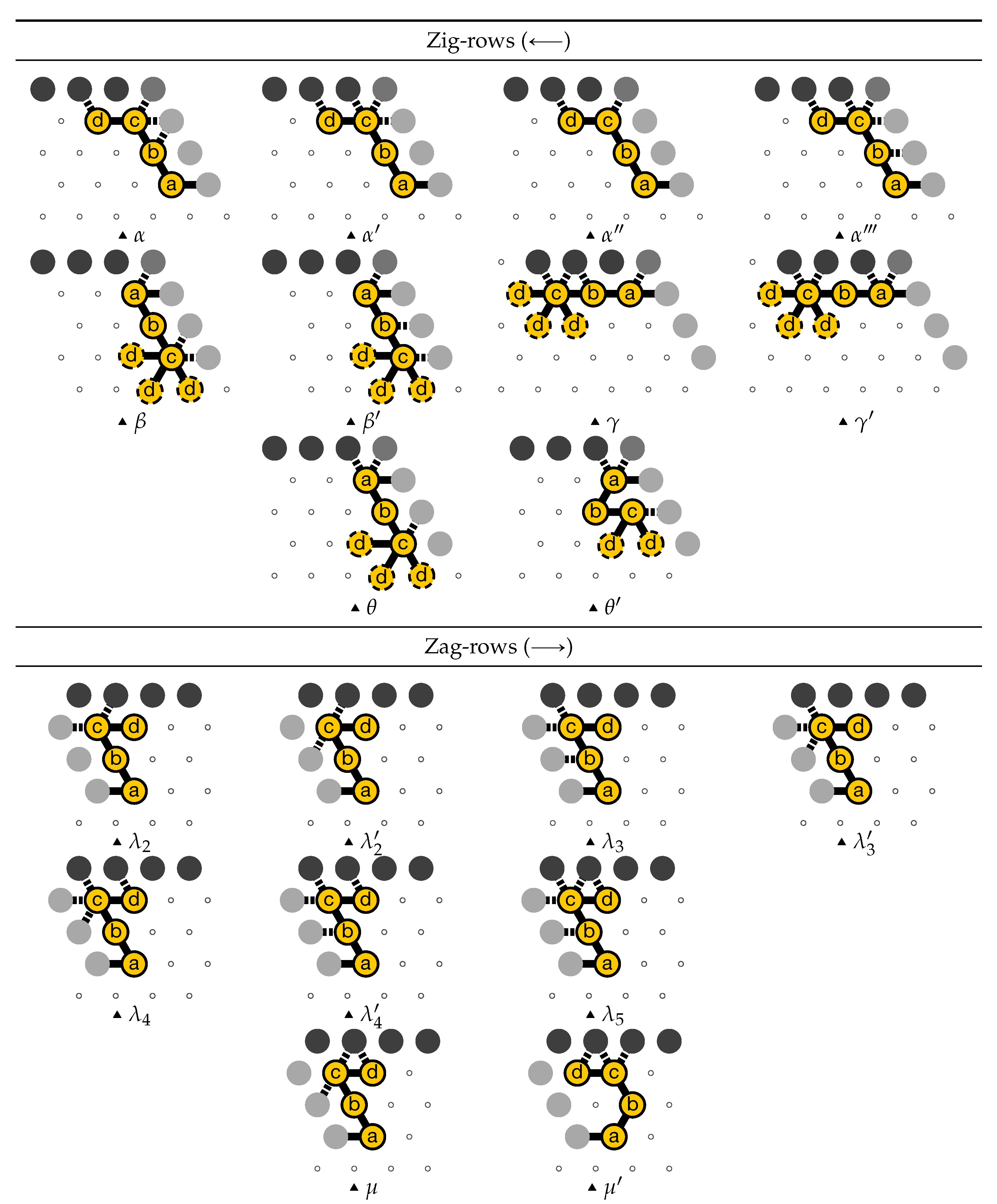
- The inner columns consist in -parallelogram regions if odd and -parallelogram regions if even. The rows consist of an alternation of Zig- and Zag-rows to be read from right to left and from left to right, respectively. The rows and take care of reading i in binary from the row above, incrementing it in row , and writing in row . In order to describe precisely the folding, let us denote by the jth lowest weight bits of when written in binary and by the position of the lowest-weight 0-bit of i: . is the position up to which the carry propagates when one increments i: . Precisely, the region in the pth inner row, and the qth inner column, is:
- -
- if is odd and is even: a -parallelogram populated with Brick , where:
- *
- if r is even, and if r is odd;
- *
- if (there still is carry to propagate), and if (there is no more carry to propagate).
- -
- if and are even: a -parallelogram populated with Brick B2 if r is even, or D2 if r is odd.
- -
- if is even and is odd: a -parallelogram populated with Brick A if r is odd and C if r is even.
- -
- if and are odd: a -parallelogram populated with Brick where:
- *
- if r is even, and if r is odd;
- *
- if (there still is carry to propagate), and if (there is no more carry to propagate).
- The seed row on top consists in the bottom row of the brick sequence BT,C0,(D2,A0,B2,C0,DT.
- The leftmost region of the last row is where the folding stops (counter capacity exceeded).
4.3. Input and Output Nascent Configurations
5. Rule Design Is NP-Hard and FPT
- Input:
- Two disjoint sets of bead types B and , a delay , k seed configurations of sequences (with possibly different lengths) and k target configurations of sequence of length n, and a dynamics .
- Output:
- A rule
![Ijms 20 02259 i001]() such that for all , the Oritatami system
such that for all , the Oritatami system ![Ijms 20 02259 i001]() , folds deterministically into the configuration from the seed configuration according to dynamics , i.e., such that: for all .
, folds deterministically into the configuration from the seed configuration according to dynamics , i.e., such that: for all .
5.1. NP-Completeness
5.2. An Efficient Algorithm in Practice
| Algorithm 1 Rule Design Problem FPT Algorithm—Oblivious dynamics |
|
| Algorithm 2 Rule Design Problem FPT Algorithm—Inertial dynamics |
|
5.3. Comparison with Related Works
6. Perspectives
Supplementary Materials
Author Contributions
Funding
Acknowledgments
Conflicts of Interest
References
- Rothemund, P.W.K. Folding DNA to create nanoscale shapes and patterns. Nature 2006, 440, 297–302. [Google Scholar] [CrossRef]
- Yurke, B.; Turberfield, A.J.; Mills, A.P.; Simmel, F.C.; Neumann, J.L. A DNA-fuelled molecular machine made of DNA. Nature 2000, 406, 605–608. [Google Scholar] [CrossRef] [PubMed]
- Evans, C.G. Crystals that Count! Physical Principles and Experimental Investigations of DNA Tile Self-Assembly. Ph.D. Thesis, California Institute of Technology, Pasadena, CA, USA, 2014. [Google Scholar]
- Seeman, N.C. Nucleic-acid junctions and lattices. J. Theor. Biol. 1982, 99, 237–247. [Google Scholar] [CrossRef]
- Winfree, E. Algorithmic Self-Assembly of DNA. Ph.D. Thesis, Caltech, Pasadena, CA, USA, 1998. [Google Scholar]
- Cannon, S.; Demaine, E.D.; Demaine, M.L.; Eisenstat, S.; Patitz, M.J.; Schweller, R.; Summers, S.M.; Winslow, A. Two Hands Are Better Than One (up to constant factors). In Proceedings of the 30th International Symposium on Theoretical Aspects of Computer Science, Kiel, Germany, 27 February–2 March 2013; pp. 172–184. [Google Scholar]
- Chen, H.L.; Doty, D. Parallelism and Time in Hierarchical Self-Assembly. In Proceedings of the 23rd Annual ACM-SIAM Symposium on Discrete Algorithms, Kyoto, Japan, 17–19 January 2012; pp. 1163–1182. [Google Scholar]
- Fujibayashi, K.; Zhang, D.Y.; Winfree, E.; Murata, S. Error suppression mechanisms for DNA tile self-assembly and their simulation. Nat. Comput. 2009, 8, 589–612. [Google Scholar] [CrossRef]
- Cook, M.; Fu, Y.; Schweller, R.T. Temperature 1 Self-Assembly: Deterministic Assembly in 3D and Probabilistic Assembly in 2D. In Proceedings of the 22nd Annual ACM-SIAM Symposium on Discrete Algorithms, San Francisco, CA, USA, 23–25 January 2011. [Google Scholar]
- Woods, D.; Doty, D.; Myhrvold, C.; Hui, J.; Zhou, F.; Yin, P.; Winfree, E. Diverse and robust molecular algorithms using reprogrammable DNA self-assembly. Nature 2019, 567, 366–372. [Google Scholar] [CrossRef] [PubMed]
- Afonin, K.A.; Bindewald, E.; Yaghoubian, A.J.; Voss, N.; Jacovetty, E.; Shapiro, B.A.; Jaeger, L. In vitro Assembly of Cubic RNA-Based Scaffolds Designed in silico. Nat. Nanotechnol. 2010, 5, 676–682. [Google Scholar] [CrossRef] [PubMed]
- Afonin, K.A.; Kireeva, M.; Grabow, W.W.; Kashiev, M.; Jaeger, L.; Shapiro, B.A. Co-transcriptional Assembly of Chemically Modified RNA Nanoparticles Functionalized with siRNAs. Nano Lett. 2012, 12, 5192–5195. [Google Scholar] [CrossRef] [PubMed]
- Li, M.; Zheng, M.; Wu, S.; Tian, C.; Weizmann, Y.; Jiang, W.; Wang, G.; Mao, C. In vivo production of RNA nanostructures via programmed folding of single-stranded RNAs. Nat. Commun. 2018, 9, 2196. [Google Scholar] [CrossRef] [PubMed]
- Schwarz-Schilling, M.; Dupin, A.; Chizzolini, F.; Krishnan, S.; Mansy, S.S.; Simmel, F.C. Optimized Assembly of a Multifunctional RNA-Protein Nanostructure in a Cell-Free Gene Expression System. Nano Lett. 2018, 18, 2650–2657. [Google Scholar] [CrossRef] [PubMed]
- Zuker, M.; Sankoff, D. RNA secondary structures and their prediction. Bull. Math. Biol. 1984, 46, 591–621. [Google Scholar] [CrossRef]
- Mathews, D.H.; Disney, M.D.; Childs, J.L.; Schroeder, S.J.; Zuker, M.; Turner, D.H. Incorporating chemical modification constraints into a dynamic programming algorithm for prediction of RNA secondary structure. Proc. Natl. Acad. Sci. USA 2004, 101, 7287–7292. [Google Scholar] [CrossRef] [PubMed]
- Mathews, D. Revolutions in RNA secondary structure prediction. J. Mol. Biol. 2006, 359, 526–532. [Google Scholar] [CrossRef] [PubMed]
- Rivas, E. The four ingredients of single-sequence RNA secondary structure prediction. A unifying perspective. RNA Biol. 2013, 10, 1185–1196. [Google Scholar] [CrossRef] [PubMed]
- Jabbari, H.; Condon, A. A fast and robust iterative algorithm for prediction of RNA pseudoknotted secondary structures. BMC Bioinform. 2014, 15, 147. [Google Scholar] [CrossRef]
- Dill, K. Theory for the folding and stability of globular proteins. Biochemistry 1985, 24, 1501–1509. [Google Scholar] [CrossRef] [PubMed]
- Unger, R.; Moult, J. Finding the lowest free energy conformation of a protein is an NP-hard problem: Proof and implications. Bull. Math. Biol. 1993, 55, 1183–1198. [Google Scholar] [CrossRef] [PubMed]
- Paterson, M.; Przytycka, T. On the complexity of string folding. In Proceedings of the 23rd International Colloquium on Automata, Languages, and Programming, Paderborn, Germany, 8–12 July 1996; Meyer, F., Monien, B., Eds.; Springer: Berlin/Heidelberg, Germany, 1996; Volume 1099, pp. 658–669. [Google Scholar]
- Atkins, J.; Hart, W.E. On the Intractability of Protein Folding with a Finite Alphabet of Amino Acids. Algorithmica 1999, 25, 279–294. [Google Scholar] [CrossRef]
- Berger, B.; Leighton, T. Protein folding in the hydrophobic-hydrophilic (HP) model is NP-complete. J. Comput. Biol. 1998, 5, 27–40. [Google Scholar] [CrossRef]
- Crescenzi, P.; Goldman, D.; Papadimitriou, C.; Piccolboni, A.; Yannakakis, M. On the complexity of protein folding. J. Comput. Biol. 1998, 5, 423–465. [Google Scholar] [CrossRef]
- Aichholzer, O.; Bremner, D.; Demaine, E.D.; Meijer, H.; Sacristán, V.; Soss, M. Long proteins with unique optimal foldings in the H-P model. Comput. Geom. 2003, 25, 139–159. [Google Scholar] [CrossRef]
- Boyle, J.; Robillardl, G.; Kim, S. Sequential folding of transfer RNA. A nuclear magnetic resonance study of successively longer tRNA fragments with a common 5′ end. J. Mol. Biol. 1980, 139, 601–625. [Google Scholar] [CrossRef]
- Frieda, K.L.; Block, S.M. Direct observation of cotranscriptional folding in an adenine riboswitch. Science 2012, 338, 397–400. [Google Scholar] [CrossRef] [PubMed]
- Geary, C.; Rothemund, P.W.K.; Andersen, E.S. A Single-Stranded Architecture for Cotranscriptional Folding of RNA Nanostructures. Science 2014, 345, 799–804. [Google Scholar] [CrossRef] [PubMed]
- Geary, C.; Chworos, A.; Verzemnieks, E.; Voss, N.R.; Jaeger, L. Composing RNA Nanostructures from a Syntax of RNA Structural Modules. Nano Lett. 2017, 17, 7095–7101. [Google Scholar] [CrossRef] [PubMed]
- Jepsen, M.D.E.; Sparvath, S.M.; Nielsen, T.B.; Langvad, A.H.; Grossi, G.; Gothelf, K.V.; Andersen, E.S. Development of a Genetically Encodable FRET System using Fluorescent RNA Aptamers. Nat. Commun. 2018, 9, 18. [Google Scholar] [CrossRef] [PubMed]
- Doty, D.; Lutz, J.H.; Patitz, M.J.; Schweller, R.T.; Summers, S.M.; Woods, D. The tile assembly model is intrinsically universal. In Proceedings of the 53rd Annual IEEE Symposium on Foundations of Computer Science, New Brunswick, NJ, USA, 20–23 October 2012; pp. 439–446. [Google Scholar]
- Meunier, P.E.; Patitz, M.J.; Summers, S.M.; Theyssier, G.; Winslow, A.; Woods, D. Intrinsic universality in tile self-assembly requires cooperation. In Proceedings of the 25th Annual ACM-SIAM Symposium on Discrete Algorithms, Portland, OR, USA, 5–7 January 2014. [Google Scholar]
- Rothemund, P.W.K.; Papadakis, N.; Winfree, E. Algorithmic Self-Assembly of DNA Sierpinski Triangles. PLoS Biol. 2004, 2, e424. [Google Scholar] [CrossRef]
- Fujibayashi, K.; Hariadi, R.; Park, S.H.; Winfree, E.; Murata, S. Toward Reliable Algorithmic Self-Assembly of DNA Tiles: A Fixed-Width Cellular Automaton Pattern. Nano Lett. 2008, 8, 1791–1797. [Google Scholar] [CrossRef]
- Wei, B.; Dai, M.; Yin, P. Complex shapes self-assembled from single-stranded DNA tiles. Nature 2012, 485, 623–626. [Google Scholar] [CrossRef]
- Geary, C.; Meunier, P.E.; Schabanel, N.; Seki, S. Programming Biomolecules That Fold Greedily During Transcription. In Proceedings of the 41st International Symposium on Mathematical Foundations of Computer Science, Krakow, Poland, 22–26 August 2016; Volume 58, p. 43. [Google Scholar]
- Masuda, Y.; Seki, S.; Ubukata, Y. Towards the Algorithmic Molecular Self-assembly of Fractals by Cotranscriptional Folding. In Proceedings of the 23rd International Conference on Implementation and Application of Automata, Charlottetown, PE, Canada, 30 July–2 August 2018; Volume 10977, pp. 261–273. [Google Scholar]
- Demaine, E.; Hendricks, J.; Olsen, M.; Patitz, M.J.; Rogers, T.A.; Nicolas, S.; Seki, S.; Thomas, H. Know When to Fold ’Em: Self-assembly of Shapes by Folding in Oritatami. In Proceedings of the 24th International Conference on DNA Computing and Molecular Programming, Jinan, China, 8–12 October 2018; Volume 11145, pp. 19–36. [Google Scholar]
- Han, Y.S.; Kim, H. Construction of Geometric Structure by Oritatami System. In Proceedings of the International Conference on DNA Computing and Molecular Programming, Jinan, China, 8–12 October 2018; Volume 11145, pp. 173–188. [Google Scholar]
- Han, Y.S.; Kim, H.; Ota, M.; Seki, S. Nondeterministic seedless oritatami systems and hardness of testing their equivalence. Nat. Comput. 2018, 17, 67–79. [Google Scholar] [CrossRef]
- Geary, C.; Meunier, P.E.; Schabanel, N.; Seki, S. Proving the Turing Universality of Oritatami Co-Transcriptional Folding. In Proceedings of the 29th International Symposium on Algorithms and Computation, Taiwan, China, 16–19 December 2018; Volume 123, p. 23. [Google Scholar]
- Ota, M.; Seki, S. Rule Set Design Problems for Oritatami Systems. Theor. Comput. Sci. 2017, 671, 26–35. [Google Scholar] [CrossRef]
- Han, Y.S.; Kim, H.; Seki, S. Transcript Design Problem of Oritatami Systems. In Proceedings of the International Conference on DNA Computing and Molecular Programming, Jinan, China, 8–12 October 2018; Volume 11145, pp. 139–154. [Google Scholar]
- Han, Y.S.; Kim, H. Ruleset Optimization on Isomorphic Oritatami Systems. In Proceedings of the 23rd International Conference on DNA Computing and Molecular Programming, Austin, TX, USA, 24–28 September 2017; Volume 10467, pp. 33–45. [Google Scholar]
- Rogers, T.A.; Seki, S. Oritatami System: A Survey and the Impossibility of Simple Simulation at Small Delays. Fund. Inform. 2017, 154, 359–372. [Google Scholar] [CrossRef]
- Woods, D.; Chen, H.L.; Goodfriend, S.; Dabby, N.; Winfree, E.; Yin, P. Active Self-Assembly of Algorithmic Shapes and Patterns in Polylogarithmic Time. In Proceedings of the ITCS 2013: Innovations in Theoretical Computer Science, Berkeley, CA, USA, 10–12 January 2013; pp. 353–354. [Google Scholar]

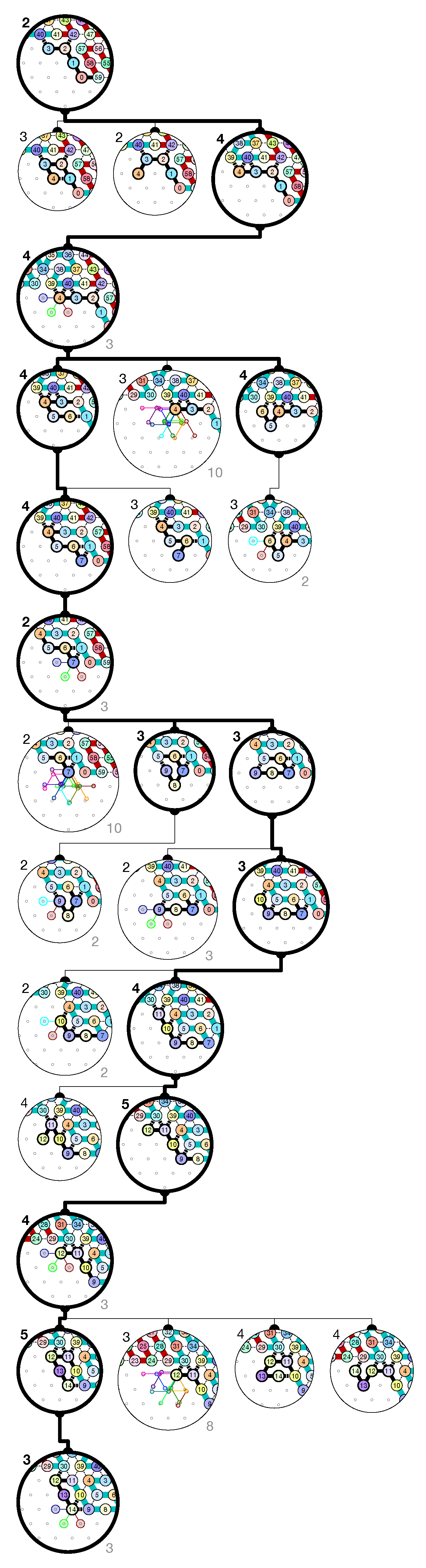
 of the Counter oritatami system: in this diagram, we have b iff there is a bullet • at the intersection of one the two lines coming from b and from ; for instance, we have 4 8 but not 4 7.
of the Counter oritatami system: in this diagram, we have b iff there is a bullet • at the intersection of one the two lines coming from b and from ; for instance, we have 4 8 but not 4 7.
of the Counter oritatami system: in this diagram, we have b iff there is a bullet • at the intersection of one the two lines coming from b and from ; for instance, we have 4 8 but not 4 7.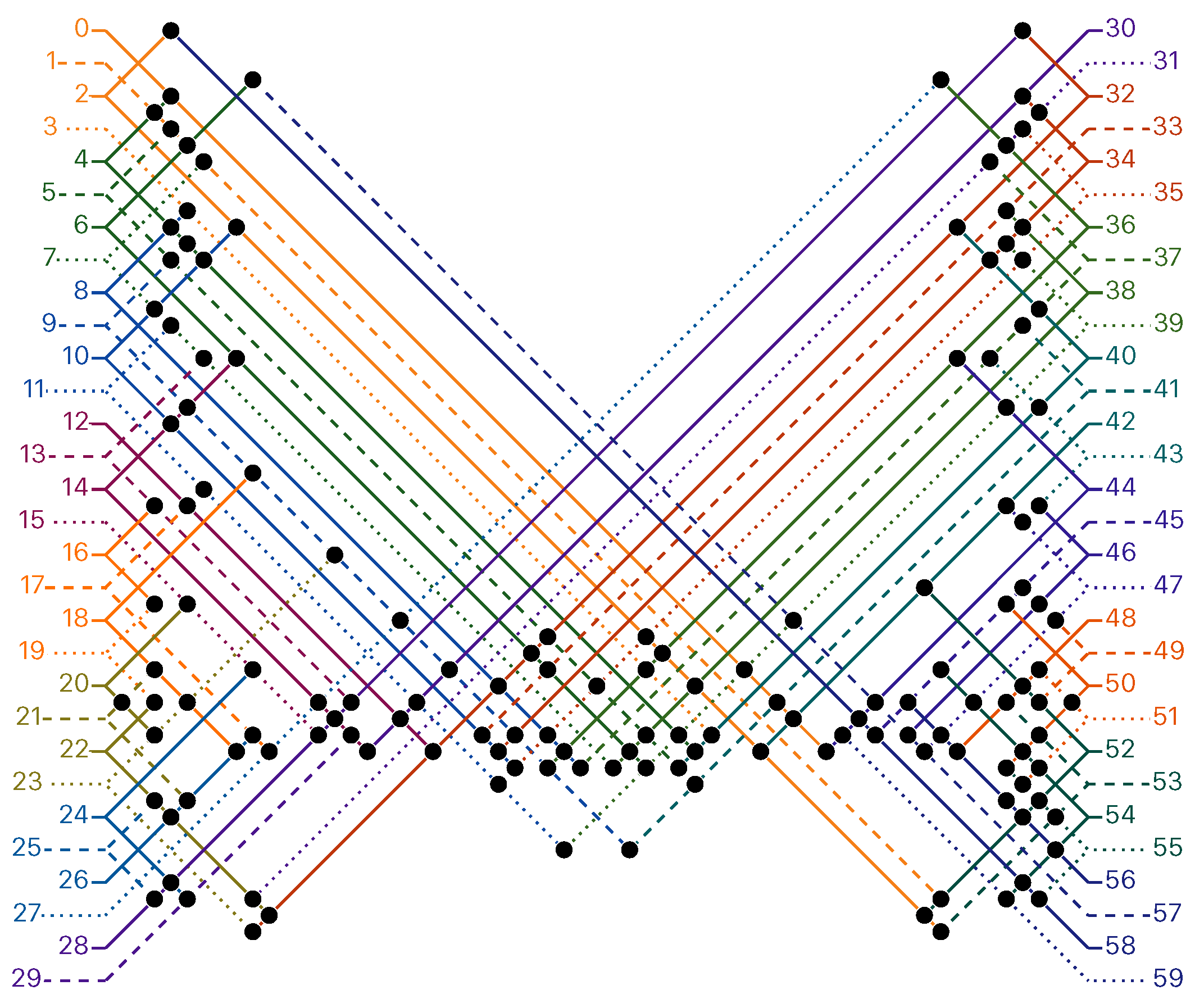


 .
.
 .
.


© 2019 by the authors. Licensee MDPI, Basel, Switzerland. This article is an open access article distributed under the terms and conditions of the Creative Commons Attribution (CC BY) license (http://creativecommons.org/licenses/by/4.0/).
Share and Cite
Geary, C.; Meunier, P.-É.; Schabanel, N.; Seki, S. Oritatami: A Computational Model for Molecular Co-Transcriptional Folding. Int. J. Mol. Sci. 2019, 20, 2259. https://doi.org/10.3390/ijms20092259
Geary C, Meunier P-É, Schabanel N, Seki S. Oritatami: A Computational Model for Molecular Co-Transcriptional Folding. International Journal of Molecular Sciences. 2019; 20(9):2259. https://doi.org/10.3390/ijms20092259
Chicago/Turabian StyleGeary, Cody, Pierre-Étienne Meunier, Nicolas Schabanel, and Shinnosuke Seki. 2019. "Oritatami: A Computational Model for Molecular Co-Transcriptional Folding" International Journal of Molecular Sciences 20, no. 9: 2259. https://doi.org/10.3390/ijms20092259
APA StyleGeary, C., Meunier, P.-É., Schabanel, N., & Seki, S. (2019). Oritatami: A Computational Model for Molecular Co-Transcriptional Folding. International Journal of Molecular Sciences, 20(9), 2259. https://doi.org/10.3390/ijms20092259