Article

Genome-Wide Correlation of 36 Agronomic Traits in the 287 Pepper (Capsicum) Accessions Obtained from the SLAF-seq-Based GWAS

1
Beijing Key Laboratory of Growth and Developmental Regulation for Protected Vegetable Crops, China Agricultural University, Beijing 100193, China
2
Department of Vegetable Science, College of Horticulture, China Agricultural University, No. 2 Yuanmingyuan Xi Lu, Haidian District, Beijing 100193, China
*
Authors to whom correspondence should be addressed.
These authors contributed equally to this work.
Int. J. Mol. Sci. 2019, 20(22), 5675; https://doi.org/10.3390/ijms20225675
Submission received: 5 October 2019 / Revised: 29 October 2019 / Accepted: 4 November 2019 / Published: 13 November 2019
(This article belongs to the Section Molecular Genetics and Genomics)

Abstract

:
There are many agronomic traits of pepper (Capsicum L.) with abundant phenotypes that can benefit pepper growth. Using specific-locus amplified fragment sequencing (SLAF-seq), a genome-wide association study (GWAS) of 36 agronomic traits was carried out for 287 representative pepper accessions. To ensure the accuracy and reliability of the GWAS results, we analyzed the genetic diversity, distribution of labels (SLAF tags and single nucleotide polymorphisms (SNPs)) and population differentiation and determined the optimal statistical model. In our study, 1487 SNPs were highly significantly associated with 26 agronomic traits, and 2126 candidate genes were detected in the 100-kb region up- and down-stream near these SNPs. Furthermore, 13 major association peaks were identified for 11 key agronomic traits. Then we examined the correlations among the 36 agronomic traits and analyzed SNP distribution and found 37 SNP polymerization regions (total size: 264.69 Mbp) that could be selected areas in pepper breeding. We found that the stronger the correlation between the two traits, the greater the possibility of them being in more than one polymerization region, suggesting that they may be linked or that one pleiotropic gene controls them. These results provide a theoretical foundation for future multi-trait pyramid breeding of pepper. Finally, we found that the GWAS signals were highly consistent with those from the nuclear restorer-of-fertility (Rf) gene for cytoplasmic male sterility (CMS), verifying their reliability. We further identified Capana06g002967 and Capana06g002969 as Rf candidate genes by functional annotation and expression analysis, which provided a reference for the study of cytoplasmic male sterility in Capsicum.

1. Introduction

The agronomic traits of pepper (Capsicum L.) have many categories with abundant phenotypes, which affect the roots, stem, leaves, flowers, and fruits [1,2,3]. Agronomic traits of pepper are closely related to pepper growth, and previous correlation and path analyses have indicated that fruit color, shape, and weight can be directly used as economic indicators and consumer purchase criteria for pepper products [4]. Plant type (Pt), branching habit (Bh), leaf shape (Ls), leaf color (Lc), first flower node (Ffn), number of flowers per axil (Nfpa), flowering date, and percentage of fertile fruit also affected the yield of pepper [5,6,7]. Stem and leaf pubescence (Lp) and dry matter, capsaicinoid, vitamin C, and anthocyanin content were correlated with resistance to disease and insect pests of pepper, which affected pepper production [8,9,10,11,12]. Therefore, mapping the genes that control agronomic traits is important for the development of the pepper industry (e.g., high-quality breeding and multi-trait pyramid breeding). However, most agronomic traits of pepper are controlled by quantitative trait loci (QTLs) and affected by environmental conditions, which makes it difficult to study these genes.
Previously, QTL mapping of agronomic traits in pepper has mainly focused on the agronomic traits closely associated with increasing pepper yield, such as fruit-related traits, disease resistance, and stress resistance (Table S1). For instance, using restriction fragment length polymorphism (RFLP), amplified fragment length polymorphism (AFLP), and random amplified polymorphic DNA (RAPD) markers, Ben Chaim et al., (2001) detected fs3.1 controlling fruit shape in an F3 population [13]. Blum et al. (2003) detected cap controlling capsaicin content on chromosome 7 in an F2 population using RAPD and sequence characterized amplified regions (SCARs) markers [14]. There have also been several reports on QTL analyses of other agronomic traits, such as Pt, Bh, Ls, leaf margin (Lm), Ffn, and Nfpa [15,16,17]. However, there were no major QTLs detected, and the genes controlling QTLs have not been characterized.
In addition, some QTLs showed a cluster distribution in rice and in pepper [17,18], suggesting that these QTLs may be controlled either by one pleotropic gene or by a group of closely linked genes. Peterson (1959) found that the A gene (controlling purple color) was linked to the sw gene (controlling green color), and that both of them were linked to the O gene (controlling oblate fruit shape) in pepper [19]. Ben Chaim et al. (2003) mapped two anthocyanin loci (Fc and A) linked to a major quantitative trait locus, fs 10.1, for fruit-shape index [20]. These studies indicated that it is necessary to analyze the distribution of genes controlling the various traits of pepper, and then to explore the relationship between the traits at the genetic level.
The traditional QTL analysis, a gene mapping method, constructs separate populations (e.g., BC1, F2, F3, recombinant inbred line, and double haploid) and then maps the genes based on mass molecular markers (e.g., RFLP, RAPD, AFLP, simple sequence repeat (SSR), cleaved amplified polymorphic sequence (CAPS), and insertion/deletion (INDEL)) (Table S1). Therefore, it is labor intensive, time consuming, and expensive, and the location accuracy is limited by the genetic diversity of the parents and the density of molecular markers used in the different populations [21,22,23]. With the rapid development of high-throughput sequencing technology, genome-wide association study (GWAS) based on linkage disequilibrium has become another powerful tool for analyzing complex agronomic traits [23]. This approach can overcome the limitations of QTL analysis and finds the association between single nucleotide polymorphisms (SNPs) and phenotype by detecting gene (locus) imbalances in natural populations [24]. This method has been successfully applied to the identification of candidate genes controlling complex agronomic traits in plant species, such as wheat, rice, maize, soya bean, chickpea, tomato, cabbage, cucumber, and alfalfa [25,26,27,28,29,30,31,32]. There have been few reports on the application of GWAS in pepper, and most experiments focused on only one or several agronomic traits. Through analyzing 96 pepper accessions by GWAS, Nimmakayala et al. (2014) found one marker on chromosome 1, which was significantly associated with capsaicin and dihydrocapsaicin content [33]. Two years later, Nimmakayala et al. (2016a, 2016b) examined the weight per fruit (Wpf) and fruit pedicel length (Fpl) by GWAS. Their results showed that there were 16 and 36 SNPs significantly associated with the Wpf and Fpl, respectively [34,35]. Ahn et al. (2018) also mapped the genes associated with powdery mildew resistance on chromosome 4 by GWAS [36].
GWAS can result in a high frequency of false positive errors for screening SNPs associated with traits [37]. Therefore, some researchers have combined traditional QTL mapping with GWAS to study the traits of arabidopsis, rice, maize, winter faba bean, and soybean [28,38,39,40,41]. Such combined approaches successfully avoid the limitations of applying the two methods separately and increase the reliability of the results. This combined strategy has also been successfully applied to pepper, with Han et al. (2018) identifying five candidate genes involved in capsaicinoid biosynthesis in the regions found by GWAS and QTL analysis [42]. However, the measures taken by these studies to improve the reliability of GWAS results were based on only one aspect (validation methods) and did not consider material population or statistical models.
For species with larger genomes, GWAS is also expensive. Specific-locus amplified fragment sequencing (SLAF-seq) is a strategy for discovering SNPs facilitated by reduced-representation genome sequencing and next-generation sequencing technologies. SLAF-seq is not only cheaper, but also obtains markers with high coverage and can be typed among populations, providing an efficient method for the detection of SNP markers in species with larger genomes, such as wheat, hulless barley, sunflower, and pepper. Three agronomic traits of pepper have been analyzed by SLAF-seq: Ffn, resistance to Phytophthora root rot, and resistance to Cucumber mosaic virus [43,44,45]. These studies demonstrated the efficiency of SLAF-seq as a strategy for the identification of SNPs (or genes) in pepper.
In our study, 36 agronomic traits were investigated in 287 pepper accessions in a GWAS (Table S2 and Note S1). The rates of false positive errors in GWAS analyses can be high owing to population structure and relatedness [22]. Therefore, the following analyses were carried out successively: (1) genetic diversity analysis to evaluate the phenotypic and genetic variation; (2) distribution analysis for SLAF tags and SNPs to assess the quality of development markers; (3) determination of optimal statistical model for each agronomic trait; (4) large-scale GWAS for the 36 agronomic traits; (5) construction of physical map based on the SNPs significantly associated with the 36 agronomic traits to explore correlations among agronomic traits; (6) verification of GWAS results based on fine mapping of male-sterility (Rf gene) traits. Our objective was to identify candidate genes controlling agronomic traits important for pepper growing and explore the correlations among the 36 traits. Our findings provide key information for breeding high-quality pepper varieties and will be useful for developing multi-trait pyramid breeding strategies and increasing pepper yield.

2. Results

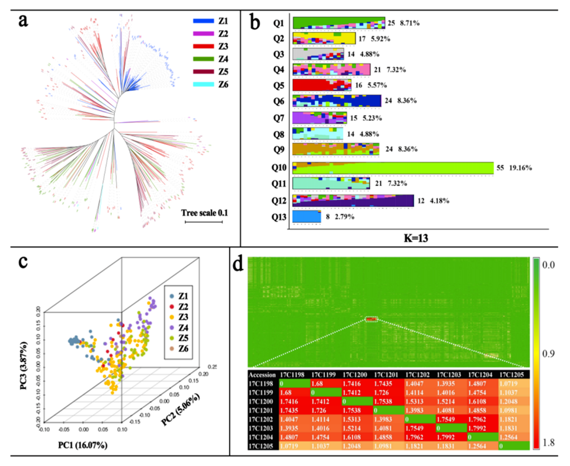
2.1. Genetic Diversity Analysis for the GWAS Population

In our study, 36 agronomic traits of pepper were surveyed and divided into 23 qualitative and 13 quantitative traits (Tables S3 and S4; Figures S1–S4). For the qualitative traits, 71 (80 in pepper germplasm resources) phenotypic types were identified, accounting for 88.75% of pepper germplasm resources (Table S3). The frequency distribution showed the main phenotype in those accessions (Figure S5). The coefficient of variation (CV) of 23 qualitative traits ranged from 0.09 to 0.74. Pt and Bh had the lowest CV (0.09), and fruit shoulder shape (Fss) had the highest CV (0.74). The Shannon Wiener index (H′) of 23 qualitative traits ranged from 0.14 (corolla color, Cc) to 1.24 (fruit surface furrow, Fsf). For the 13 quantitative traits, the frequency of Ffn, Fpl, and fruit length (Fl) were normally distributed (Figure S6). However, the frequency distribution of the other quantitative traits was positively skewed, indicating that a large proportion of the 287 pepper accessions had a lower value for these traits (Figure S6). In addition, mode, mean, min, max, range, CV, and H′ were used to assess the variation in quantitative traits (Table S4). The CV of 13 quantitative traits ranged from 0.26 (Fpl) to 1.07 (Wpf). The H′ of 13 quantitative traits ranged from 0.45 (Nfpa) to 2.01 (Fl). Our results confirmed that most of the 36 agronomic traits had a rich phenotypic variation, suggesting that this population met the requirements for GWAS analysis.

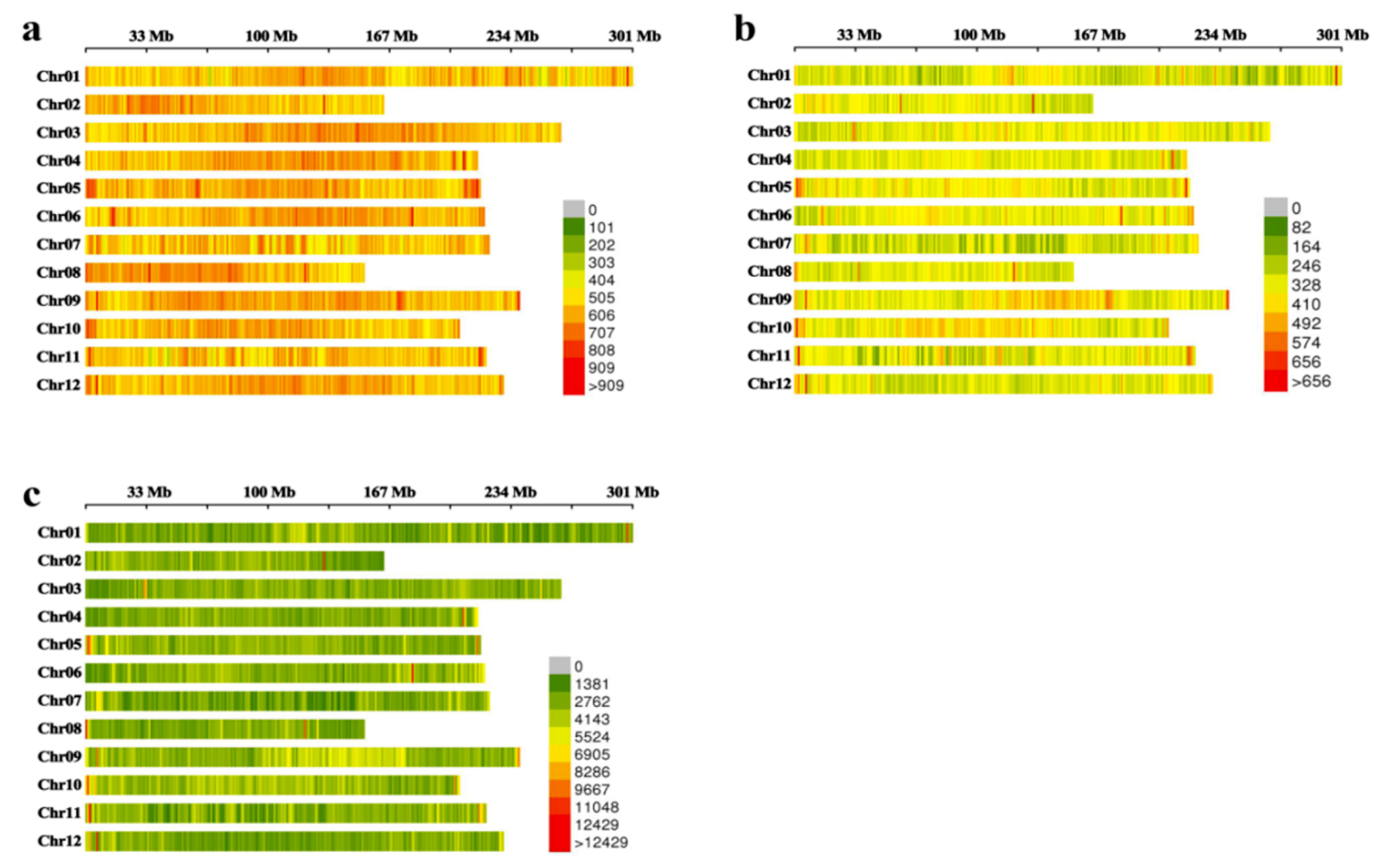
2.2. Identification and Distribution Analysis for Labels

In total, 2238.81 M paired-end reads were obtained from 287 pepper accessions based on HaeIII digestion. The average value of Q30 (Q30 indicates a quality score of 30, indicating a 0.1% error rate or 99.9% sequence accuracy) and GC content were 95.72% (93.62–96.6%) and 39.30% (38.51–42.42%), respectively, indicating that our sequencing results for 287 pepper accessions were reliable (Table S5). Further analysis revealed that 1,824,874 SLAF tags were obtained, with 287,910–475,273 tags for each accession. The average sequencing depth of each accession was different (12.17–44.22; average, 19.62) but met the assumptions of the SLAF test (Table S6). Furthermore, 1,025,395 polymorphic SLAF tags were identified from 1,824,874 SLAF tags, and then a total of 9,557,790 SNPs were also developed from polymorphic SLAF tags (see Table S7 for SNP details).
To analyze the distribution of genetic information of SLAF tags and SNPs in the 287 accessions, we divided all accessions into 17 grades according to SLAF tag number, SNP number, SNP integrity, and SNP heterozygosity ratio (Table S8). In the population, both SLAF tags and SNPs were normally distributed (Figure S7). The eighth SLAF tag grade (SLAF tags ranged from 365,060 to 376,081) had the highest frequency (95) and percentage (33.10%). The ninth SNP grade (SNPs ranged from 3,859,505 to 3,928,957) had the highest frequency (55) and percentage (19.16%). SNP integrity was also normally distributed. These results showed that SLAF tags and SNPs were evenly distributed in the population, implying that their genetic information covered most of the accessions. However, the distribution of SNP heterozygosity ratio was positively skewed in the population, indicating that most of the accessions had a lower heterozygosity ratio.
As shown in Figure S8 and Figure 1, the distribution of SLAF tags and SNPs on chromosomes were also analyzed in our study. The percentage of polymorphic SLAF tags on every chromosome was over 50% of the total number of SLAF tags, and the percentage on chromosomes 5, 9, and 10 was high at 58.63%, 60.48%, and 63.46%, respectively. Chromosome 8 had the lowest percentage of polymorphic SLAF tags (53.13%) (Figure S8). The density thermal map of SLAF tags and polymorphic SLAF tags had fewer color types and balanced distribution (Figure 1). Similar results were observed in the density heat map of SNPs, with only a small number of regions exhibiting high density. These results suggested that all SLAF tags, polymorphic SLAF tags, and SNPs were evenly distributed on every chromosome. This reduced the probability of missing important information on different chromosomes, suggesting that theses labels can represent the genetic information of the whole pepper genome and be used for GWAS analysis of the agronomic traits of pepper.

2.3. Population Structure Analysis for the GWAS Population

In the present study, linkage disequilibrium was calculated for every chromosome using 594,429 SNPs (integrity >0.5; minor allele frequency (MAF) > 0.05). Squared correlations of allele frequencies (R2) were used to investigate the extent of LD calculated within a 0–500-kb window. As shown in Figure S9, the LD decay distance for the 287 pepper accessions between all SNPs was >500 kb when the value of the cut-off for R2 was set at 0.1, which showed that there was a greater probability of linkage among those SNPs in the accessions. In addition, the LD decays were not evenly distributed among chromosomes within the 0–500-kb window. However, obvious LD differentiation was found among chromosome 1 and the other chromosomes.
Population structure and relatedness were the major factors leading to high rates of false positive errors in GWAS analysis [22]. Therefore, three methods were used to assess the population. First, a phylogenetic tree was constructed. As shown in Figure 2a, 287 pepper accessions were divided into four large categories and seven subcategories. Second, principal component analysis (PCA) was carried out. The interpretation rates of the first three principal components were 16.07% (PC1), 5.06% (PC2), and 3.87% (PC3), and cumulative variation was 25.01% (Figure S10a). The PCA triplot showed that most accessions were scattered except for one subgroup (Figure 2b, Gif S1). Third, admixture software was used to calculate the clustering from K = 1–15. As shown in Figure S10b, as the K value increased, the cross validation error rate rapidly decreased, the first valley value appeared at K = 11, the second valley value occurred at K = 13, and then the cross validation error rate increased gradually as K value increased. By comparing the value of cross validation error rate between K = 11 and K = 13, it was determined that K = 13, which had a lower cross validation error rate, was the optimal subgroup number for this population. Detailed information of the subgroups for K = 13 is shown in Figure 2c and Table S9. These results indicated a moderate level of population differentiation within different pepper subgroups.
As shown in Figure S10c, the relatedness of most accessions (76.44%) was <0.1 and was only >0.4 for 1.39% of accessions. The thermogram of relatedness also showed similar results with only eight accessions having a relatedness of >1.05 (Figure 2d). These results showed that most of the accessions were only distantly related, and thus, relatedness barely interfered with the GWAS analysis.

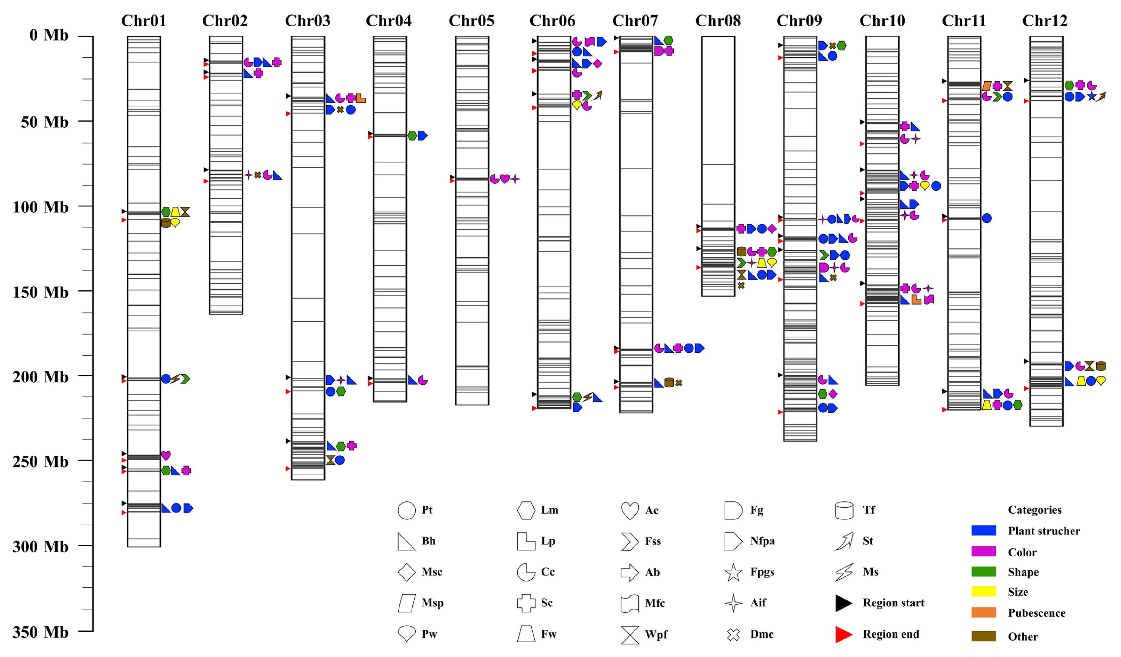
2.4. Large-Scale GWAS for 36 Agronomic Traits

The highly consistent filtered SNPs (594,429) in the 287 pepper accessions were used for GWAS analysis of 36 agronomic traits. To reduce the influence of population structure and increase the reliability of GWAS results, we used five statistical models: general linear model (GLM), mixed linear model (MLM), compressed mixed linear model (CMLM), efficient mixed-model association expedited (EMMAX), and factored spectrally transformed linear mixed model (FaST-LMM). Performance of the five models was compared based on Q-Q plots (Figures S11–S14), and the most appropriate statistical model for each trait was selected for subsequent GWAS analysis. As shown in Table 1, Fast-LMM was the optimal model of 20 traits; EMMAX was the optimal model of 11 traits; GLM was the optimal model of five traits. These results showed the optimal model of different traits can be different, implying that it was necessary for each trait to select one optimal model for GWAS analysis.
In total, 1487 SNPs were identified with p < 1.707 × 10⁻⁸ as the highly significant threshold from the optimal models, and 2126 candidate genes in the 100-kb region up- or down-stream near those SNPs were detected for 26 traits (Table S10) [46,47]. The number of highly significant associated SNPs and genes for each trait and chromosome varied (Table S11). In addition, 247 associated peaks (SNPs were arranged neatly with a columnar distribution, Figures S15–S20) were identified for the 36 traits, and the 109 associated peaks above the highly significant threshold (blue lines in Manhattan plots) were defined as significant peaks (strong association signals) for 26 traits. According to the number and physical location of SNPs in the significant peaks, 91 significant peak regions were identified for 22 traits (Table 1). The important SNPs and genes in the significant peak regions were highlighted in red (Table S10), and the important genes were annotated (Table S12).

2.4.1. The Three Stem-Related Traits

Plant Type

In total, 104 SNPs (184 genes) mainly distributed on chromosomes 1–9, 11, and 12 were significantly associated with Pt (Table S11). Chr11_37287718, Chr04_214680400, and Chr09_169528955 were the most highly associated with Pt (Table S10). Nineteen SNP polymerization regions were highlighted on chromosomes 1, 3, 6, 7, 8, 9, 11, and 12, in which the SNP associated with Pt and the SNP associated with the other traits had polymerization (Figure 3). Specifically, Pt and Bh, Pt and Cc, and Pt and Nfpa had 15, 16, and 13 polymerization regions, respectively (Table S17). Moreover, 10 highly significant peaks associated with Pt were observed on chromosomes 1, 5–7, 9, and 11, with no main peak evident (Figure S15). Furthermore, nine significant peak regions (total size: 17.19 Mbp), distributed on chromosomes 1, 4, 5, 6, 9, and 11 were identified for Pt (Table 1).

Branching Habit

In total, 307 SNPs (548 genes) distributed on all chromosomes were significantly associated with Bh (Table S11). Chr10_51277133, Chr03_240589834, and Chr10_99038533 were the most highly associated with Bh (Table S10). Then, 27 SNP polymerization regions were highlighted on chromosomes 1–4 and 6–12, in which the SNP associated with Bh and the SNP associated with the other traits had polymerization (Figure 3). Specifically, Bh and Lm, Bh and Cc, Bh and style color (Sc), Bh and Nfpa, and Bh and Aif had 9, 18, 12, 18, and 9 polymerization regions, respectively (Table S17). Moreover, eight highly significant peaks associated with Bh were observed on chromosomes 1–3, 6, 7, and 9, with no main peak evident (Figure S15). Furthermore, eight significant peak regions (total size: 20.92 Mbp), distributed on chromosomes 1, 2, 3, 6, 7, and 9, were identified for Bh (Table 1).

Main Stem Pubescence

In total, 22 SNPs (two genes) mainly distributed on chromosome 11 were significantly associated with main stem pubescence (Msp) (Table S11). Chr11_27217603, Chr11_27217695, and Chr11_27217636 were the most highly associated with Msp (Table S10). One SNP polymerization region was highlighted on chromosome 11, in which the SNP associated with Msp and the SNP associated with the other traits (Cc, Sc, Fss, and Wpf) had polymerization (Figure 3). Moreover, one highly significant peak on chromosome 11 was the main peak associated with Msp (Figure S19). Furthermore, one significant peak region (size: 1.57 Mbp), located on chromosome 11, was identified for Msp (Table 1).

2.4.2. The Two Leaf-Related Traits

Leaf Margin

In total, 117 SNPs (247 genes) mainly distributed on chromosomes 1 and 3–12 were significantly associated with Lm (Table S11). Chr09_213296577, Chr08_134733299, and Chr10_59043555 were the most highly associated with Lm (Table S10). Twelve SNP polymerization regions were highlighted on chromosomes 1, 3, 4, 6, 7, 8, 9, 11, and 12, in which the SNP associated with Lm and the SNP associated with the other traits had polymerization (Figure 3). Specifically, Lm and Cc, Lm and Sc, and Lm and Nfpa had 4, 6, and 8 polymerization regions, respectively (Table S17). Moreover, five highly significant peaks were observed on chromosomes 1, 4, 6, 8, and 12, with no main peak evident (Figure S17). Furthermore, five significant peak regions (total size: 11.18 Mbp), distributed on chromosomes 1, 4, 6, 8, and 12 were identified for Lm (Table 1).

Leaf Pubescence

In total, 17 SNPs (51 genes) mainly distributed on chromosomes 2, 3, 9, 10, and 12 were significantly associated with Lp (Table S11). Chr10_154508628, Chr09_178710956, and Chr10_197927729 were the most highly associated with Lp (Table S10). Two SNP polymerization regions were highlighted on chromosomes 3 and 10, in which the SNP associated with Lp and the SNP associated with the other traits had polymerization (Figure 3). Specifically, Lp and Cc, and Lp and Sc had two polymerization regions, respectively (Table S17). Moreover, three highly significant peaks were observed on chromosomes 10 and 12, with the former being the main peak associated with Lp (Figure S19). Furthermore, three significant peak regions (total size: 3.00 Mbp), distributed on chromosomes 10 and 12, were identified for Lp (Table 1).

2.4.3. The Five Flower-Related Traits

Corolla Color

In total, 125 SNPs (279 genes) distributed on all of chromosomes were significantly associated with Cc (Table S11). Chr02_85429287, Chr09_201616976, and Chr08_138467669 were the most highly associated with Cc (Table S10). Then, 22 SNP polymerization regions were highlighted on chromosomes 2–12, in which the SNP associated with Cc and the SNP associated with the other traits had polymerization (Figure 3). Specifically, Cc and Sc, Cc and Nfpa, and Cc and Aif had 11, 15, and 9 polymerization regions, respectively (Table S17). Moreover, eight highly significant peaks were observed on chromosomes 2, 4, 6–9, and 11, with no main peak evident (Figure S16). Furthermore, nine significant peak regions (total size: 8.18 Mbp), distributed on chromosomes 2, 4, 6, 7, 8, 9 and 11, were identified for Cc (Table 1).

Style Color

In total, 291 SNPs (152 genes) distributed on all of chromosomes were significantly associated with Sc (Table S11). Chr10_157424507, Chr10_155327941, and Chr10_155327958 were the most highly associated with Sc (Table S10). Sixteen SNP polymerization regions were highlighted on chromosomes 1, 2, 3, 6, 7, 8, 10, 11, and 12, in which the SNP associated with Sc and the SNP associated with the other traits had polymerization (Figure 3). Specifically, Sc and Nfpa, Sc and Aif had 8 and 4 polymerization regions, respectively (Table S17). Moreover, six highly significant peaks were observed on chromosomes 1–3, 8, 10, and 11, with the latter two being the main peaks associated with Sc (Figure S16). Furthermore, three significant peak regions (total size: 1.81 Mbp), distributed on chromosomes 1, 10, and 11, were identified for Sc (Table 1).

Number of Flowers Per Axil

In total, 126 SNPs (221 genes) distributed on all of chromosomes were significantly associated with Nfpa (Table S11). Chr12_193629045, Chr12_193629029, and Chr12_193628684 were the most highly associated with Nfpa (Table S10). Then, 21 SNP polymerization regions were highlighted on chromosomes 1–4 and 6–12, in which the SNP associated with Nfpa and the SNP associated with the other traits had polymerization (Figure 3). Specifically, Nfpa and Aif, Nfpa and dry matter content (Dmc) had 6 and 4 polymerization regions, respectively (Table S17). Moreover, 11 highly significant peaks were observed on chromosomes 1, 4–7, 9–10, and 12, with the latter being the main peak associated with Nfpa (Figure S15). Furthermore, 12 significant peak regions (total size: 18.48 Mbp), distributed on chromosomes 1, 4, 5, 6, 7, 9, 10, 11, and 12, were identified for Nfpa (Table 1).

Flower Pedicel Growing State

In total, 16 SNPs (14 genes) distributed on chromosome 12 were significantly associated with flower pedicel growing state (Fpgs) (Table S11). Chr12_37932067, Chr12_37994286, and Chr12_37994288 were the most highly associated with Fpgs (Table S10). One SNP polymerization region was highlighted on chromosome 12, in which the SNP associated with Fpgs and the SNP associated with the other traits (Lm, Sc, Cc, Pt, Nfpa, and spicy type (St)) had polymerization (Figure 3). Moreover, one highly significant peak on chromosome 12 was the main peak associated with Fpgs (Figure S15). Furthermore, one significant peak region (size: 5.14 Mbp), located on chromosome 12, was identified for Fpgs (Table 1).

Male Sterility

In total, 78 SNPs (17 genes) mainly distributed on chromosomes 1, 6, 10, and 11 were significantly associated with male sterility (Ms) (Table S11). Chr06_215261283, Chr06_215468191, and Chr06_215411595 were the most highly associated with Ms (Table S10). Two SNP polymerization regions were highlighted on chromosomes 1 and 6, in which the SNP associated with Ms and the SNP associated with the other traits had polymerization (Figure 3). Moreover, one highly significant peak on chromosome 6 was the main peak associated with Ms (Figure S20). Furthermore, one significant peak region (size: 1.09 Mbp), located on chromosome 6, was identified for Ms (Table 1).

2.4.4. The Five Fruit-Related Traits

Anthocyanin on Immature Fruit

In total, 102 SNPs (96 genes), mainly distributed on chromosomes 1–5 and 7–10, were significantly associated with anthocyanin on immature fruit (Aif) (Table S11). Chr07_105839253, Chr10_75362680, and Chr10_107762896 were the most highly associated with Aif (Table S10). Ten SNP polymerization regions were highlighted on chromosomes 2, 3, 5, 9, and 10, in which the SNP associated with Aif and the SNP associated with the other traits had polymerization (Figure 3). Specifically, Aif and Fss, Aif and placenta width (Pw), and Aif and Dmc had 2, 2, and 3 polymerization regions, respectively (Table S17). Moreover, seven highly significant peaks were observed on chromosomes 2, 4, and 7–10, with the latter being the main peak associated with Aif (Figure S16). Furthermore, four significant peak regions (total size: 7.59 Mbp), distributed on chromosomes 8, 9, and 10, were identified for Aif (Table 1).

Mature Fruit Color

In total, 16 SNPs (49 genes) distributed on chromosome 6 were significantly associated with mature fruit color (Mfc) (Table S11). Chr06_10060744, Chr06_8776355, and Chr06_8769243 were the most highly associated with Mfc (Table S10). Two SNP polymerization regions were highlighted on chromosomes 6 and 10, in which the SNP associated with Mfc and the SNP associated with the other traits had polymerization (Figure 3). Moreover, one highly significant peak on chromosome 6 was the main peak associated with Mfc (Figure S16). Furthermore, one significant peak region (size: 6.30 Mbp), located on chromosome 6, was identified for Mfc (Table 1).

Spicy Type

In total, 44 SNPs (29 genes) mainly distributed on chromosomes 3, 4, 9, 10, and 12 were significantly associated with St (Table S11). Chr12_35372851, Chr12_35623982, and Chr12_35624024 were the most highly associated with St (Table S10). Two SNP polymerization regions were highlighted on chromosomes 6 and 12, in which the SNP associated with St and the SNP associated with the other traits had polymerization (Figure 3). Moreover, six highly significant peaks were observed on chromosomes 3, 4, 9, 10, and 12, with the latter being the main peak associated with St (Figure S20). Furthermore, six significant peak regions (total size: 8.22 Mbp), distributed on chromosomes 4, 5, 6, 10, and 12, were identified for St (Table 1).

Placenta Width

In total, seven SNPs (18 genes) distributed on chromosomes 1, 6, 8, and 12 were significantly associated with Pw (Table S11). Chr12_206591342, Chr06_40911519, and Chr08_133396929 were the most highly associated with Pw (Table S10). Five SNP polymerization regions were highlighted on chromosomes 1, 6, 8, 10 and 12, in which the SNP associated with Pw and the SNP associated with the other traits had polymerization (Figure 3). Specifically, Pw and fruit width (Fw), Pw and Wpf, and Pw and thickness of flesh (Tf) each had three polymerization regions (Table S17). Moreover, four highly significant peaks were observed on chromosomes 1, 8, and 12, and two of them (on chromosomes 8 and 12) were the main peaks associated with Pw (Figure S18). Furthermore, two significant peak regions (total size: 3.27 Mbp), distributed on chromosomes 8 and 12, were identified for Pw (Table 1).

Fruit Width

In total, 26 SNPs (65 genes) distributed on chromosomes 1, 4, 8, and 12 were significantly associated with Fw(Table S11). Chr08_133396929, Chr08_133433188, and Chr08_133185108 were the most highly associated with Fw (Table S10). Four SNP polymerization regions were highlighted on chromosomes 1, 8, 11, and 12, in which the SNP associated with Fw and the SNP associated with the other traits had polymerization (Figure 3). Specifically, Fw and Wpf, and Fw and Tf each had three polymerization regions (Table S17). Moreover, four highly significant peaks were observed on chromosomes 1, 4, 8, and 12, with the peak on chromosome 8 being the main peak associated with Fw (Figure S18). Furthermore, three significant peak regions (total size: 6.68 Mbp), distributed on chromosomes 1, 8, and 12, were identified for Fw (Table 1).
There were few to no SNPs significantly associated with the remaining 21 traits: main stem color (Msc), Ls, Lc, leaf surface characteristics (Lsc), Ffn, anther color (Ac), fruit glossy (Fg), Fsf, fruit surface characteristics (Fsc), Fss, appendage at blossom-end (Ab), Fpl, placenta length (Pl), Fl, fruit apex shape (Fas), fruit shape index (Fsi), placenta size index (Psi), Wpf, Dmc, Tf, and number of locules (Nol). However, there were many peaks with relatively small effects observed distributed on multiple chromosomes (Figures S15–S18, S20). These findings implied that these traits may be controlled by multiple micro-genes.

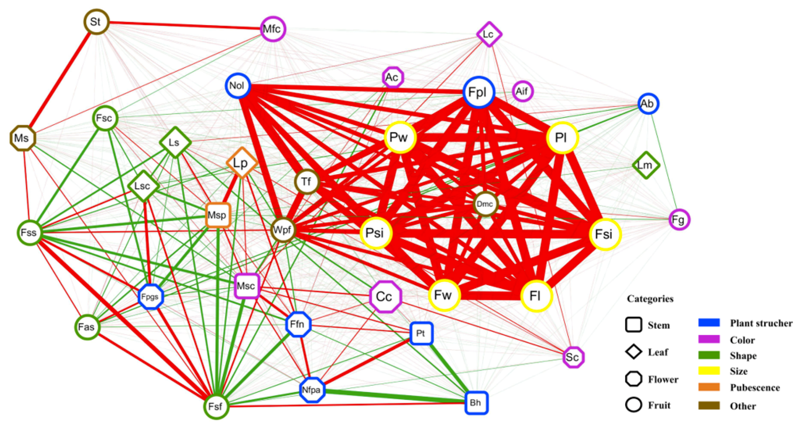
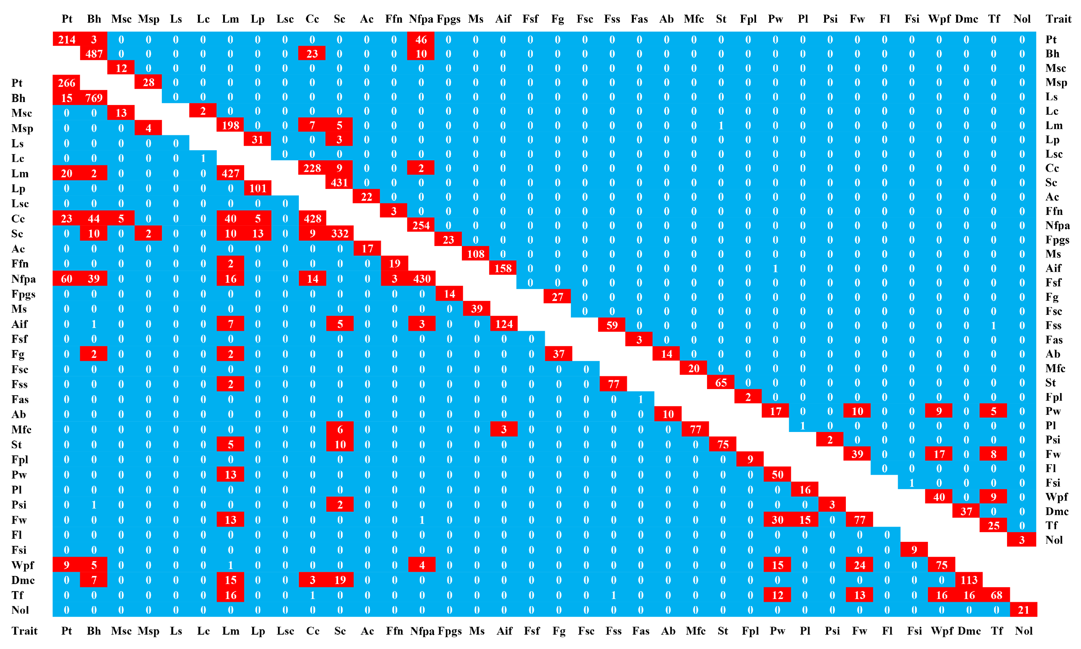
2.5. Global Exploration of Correlations Among the 36 Agronomic Traits

We explored the correlations among the 36 traits using correlation network analysis (Figure 4). The strongest positive correlation was observed among the 11 fruit-related traits: Fpl, Pw, Pl, Psi, Fw, Fl, Fsi, Nol, Wpf, Tf, and Dmc. For stem-related traits, Bh was negatively correlated with Pt (−0.49), and Msc was positively correlated with Msp (0.25) and Pt (0.23). Correlations among leaf-related traits and flower-related traits were less significant than those among stem-related traits. Correlation coefficients among pairwise traits are shown in Table S14.
We compared their shared peak numbers in Manhattan plots based on descriptive classifications (Figures S15–S20). For plant structure-related traits, Pt, Bh, and Nfpa had a total of three shared peaks distributed on chromosomes 1, 6, and 7. However, there was one shared peak on chromosome 2 for Bh and Fpgs, and one shared peak on chromosome 12 for Fpl and Fpgs.
For color-related traits, Cc and Msc, and Cc and Fg each had one shared peak distributed on chromosomes 9 and 8, respectively. Cc, Lc, and Fg had one shared peak on chromosome 12. Cc, Ac, and Aif had one shared peak on chromosome 2. Sc and Msc had one shared peak on chromosomes 8 and 10, respectively. Sc, Aif, and Mfc had one shared peak on chromosome 10. Ac and Aif had one shared peak on chromosomes 4 and 7, respectively. Msc and Mfc had one shared peaks on chromosomes 10.
For shape-related-traits, Ls and Lsc had one shared peak on chromosome 6. Ls and Fas had four shared peaks distributed on chromosomes 1, 2, 10, and 12. Moreover, Fsc and Fsf, and Fsc and Fas each had one shared peak on chromosomes 10 and 12, respectively.
For organ size-related traits, Fw and Pw had four shared peaks on chromosomes 1, 4, 8, and 12. Fl and Pl had two shared peaks distributed on chromosomes 6 and 8. Fsi and Psi had one shared peak on chromosomes 2 and 7, respectively.
For pubescence-related traits, Msp and Lp had one shared peak on chromosome 10, and it was the main peak of Lp. However, the main peak of Msp was on chromosome 11, suggesting that the major genes controlling the two traits may be different. There were more peaks for Lp (eight) than Msp (two), implying that Lp was controlled by minor genes.
For other traits, there were six shared peaks between Wpf and Tf on chromosomes 1, 3, 5, 8, 11, and 12. St and Tf had one shared peak on chromosomes 3 and 8, respectively. St and Dmc, and St and Ms each had one shared peak each on chromosomes 6 and 2, respectively. We compared the distribution of peaks of the traits between the different categories and observed one or two shared peaks for Sc and Fsf (chromosome 10), Sc and Fss (chromosomes 8 and 11), Fas and Fg (chromosome 12), and St and Fpgs (chromosome 12). It was worth noting that Sc, Fss, and Msp had one shared peak (chromosome 11), that Sc, Aif, and Lp had one shared peak (chromosome 10), and that Sc, Cc, Fw, and Pw had one shared peak (chromosome 08).
Additionally, we identified the significant SNPs near peaks for pairwise traits and summarized the SNP and gene numbers. As shown in Figure 5, we found that among the significant SNPs, some of them were associated with more than one trait. For instance, 46 SNPs (60 genes) were associated with Pt and Nfpa, and 10 SNPs (39 genes) were associated with Bh and Nfpa. Based on pairwise traits, 385 genes were associated with more than one trait, indicating gene pleiotropy. For detailed information, see Table S15.
To further confirm the relationships among agronomic traits at the whole genome level, 2526 significant SNPs (p < 1.707 × 10⁻⁷) were mapped independently on chromosomes 1–12. We found that some of the SNPs clustered in a small region on a chromosome, which was deemed to be an SNP polymerization region. Totally, 37 SNP polymerization regions (total size: 264.69 Mbp) were found in the study, which could be selected areas in pepper breeding (Table S16). As shown in Figure 3, most SNP polymerization regions were distributed on chromosomes 1, 6, 9, and 10. The polymerization regions associated with more than four traits were mainly distributed on chromosomes 6–12 (Table S16). Compared with the correlation analysis results, we found that the stronger the correlation between two traits, the greater the possibility of them being in more than one polymerization region, and the higher the number of SNPs and genes in the same polymerization region (Figure 3, Figure 4 and Figure 5 and Table S17). For example, Bh and Nfpa were negatively correlated (−0.59), and there were 18 different shared regions for them. Similar features were also found between Pt and Nfpa (16 regions), and Pt and Bh (15 regions) (Table S17).

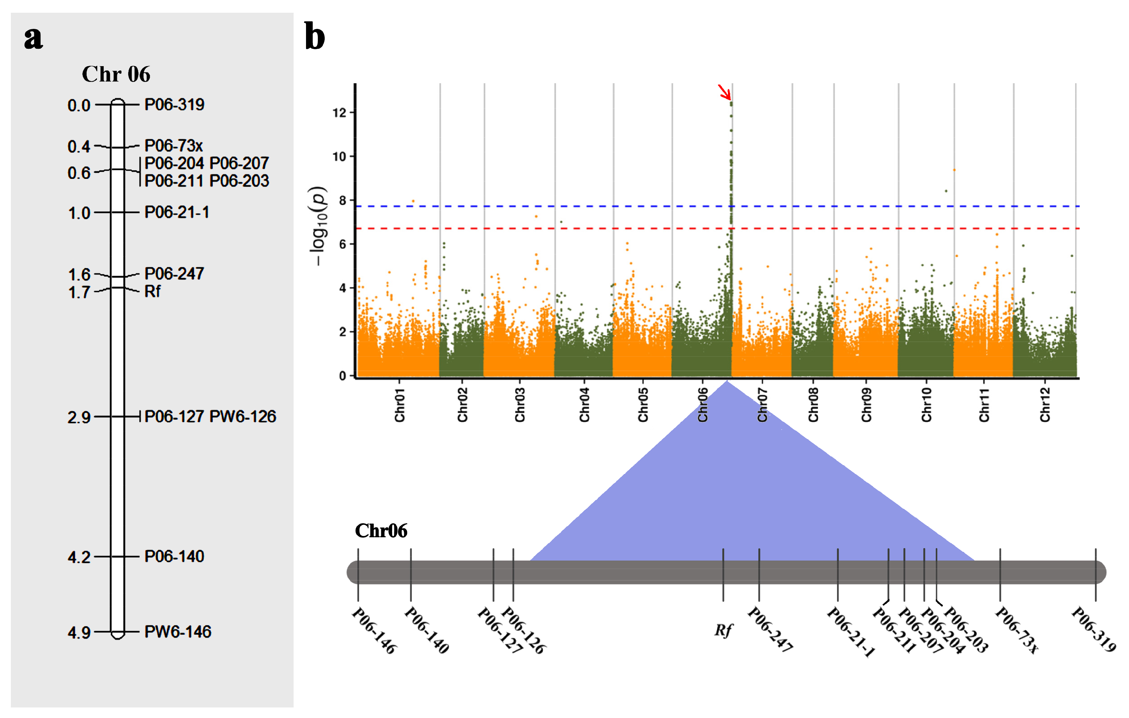
2.6. Verification of GWAS Results Based on Fine Mapping of Male-Sterility (Rf) Gene

To verify the GWAS signals, we used molecular mapping of the Rf gene for cytoplasmic male sterility. In the F2 population of 2016, 255 individuals were fertile, and 79 were sterile. A chi-squared test revealed that the ratio of fertile:sterile individuals in this population was 3:1. The Rf gene was initially mapped within 4.9 cM between the SSR markers P06-319 and PW6-146 (Figure 6a), with a physical distance of 1.8 Mb. In the F2 population of 2017, the recombinant single strains were screened with P06-319 and PW6-146 as two side markers, and 116 individuals were recombinant between these markers. Genotypic assay of the recombinants was performed using 10 SSR markers between P06-319 and PW6-146. Finally, the Rf gene was mapped to a region between the markers P06-247 and PW6-126. This region lies within 214,868,888–215,727,145 bp of chromosome 6 in the ‘Zunla-1′ genome, with a physical distance of 858,257 bp. Comparing the regions of molecular mapping with the GWAS signals, we found that the region of molecular mapping (214,868,888–215,727,145) was highly consistent with that of GWAS (214,443,037–215,536,517) (Figure 6b), which indicated that the GWAS signals were reliable.
According to Rf gene localization, the 214,868,888–215,727,145-bp region of the ‘Zunla-1’ genome was annotated, and eight genes were found in this region (Table S13). cDNA of 138A and 138C were used as templates to detect whether there were differences in the coding sequences of the genes. The sequencing results showed that there were no differences in the coding sequences of the eight genes between the two templates.
The results of expression analysis showed that no expression was detected for Capana06g002963 and Capana06g002971. Capana06g002965 was expressed in both anthers and leaves, and its expression in anthers gradually decreased with bud development but showed no significant difference between 138A and 138C (Figure S21a). Capana06g002967 was mainly expressed in buds, and the expression level gradually increased with bud development. The expression level of 138C was significantly higher than that of 138A at all stages of bud development (Figure S21b). Capana06g002968 was mainly expressed in buds, and the highest expression was found in the anthers of 138A at the mature stage (Figure S21c). Capana06g002969 was expressed in both anthers and leaves, and the anther expression in all stages of 138C was significantly higher than that in 138A (Figure S21d). Capana06g002970 was expressed in both anthers and leaves, but there was no significant difference between 138A and 138C (Figure S21e). Capana06g002972 was expressed in both anthers and leaves, and the highest expression was in the anthers of 138C at maturity and was significantly higher than that of 138A (Figure S21f). Based on the results, Capana06g002967 and Capana06g002969 were identified as Rf candidate genes.

3. Discussion

There are many agronomic traits with abundant phenotypes in pepper. However, most of the previous studies on the gene mapping of agronomic traits in pepper were based on the traditional QTL mapping method, and only a single or several traits were studied in the same study [48,49,50,51]. Although, there are also reports of the use of GWAS in pepper, most of this research was only focused on one or two traits [33,43,52]. In our study, the GWAS of 36 agronomic traits was carried out at the same time. A large number of SNP loci significantly associated with agronomic traits were obtained, and the main correlation peaks of some key agronomic traits were identified. Our results showed that GWAS could be used to study multiple agronomic traits in the same study, which greatly improved the efficiency of gene mapping of agronomic traits in pepper.
However, GWAS does have the potential for false positive errors due to the population structure, relatedness, and inappropriate statistical models [22,37,53,54]. From previous studies, we summarized three aspects that may contribute to improving the accuracy of GWAS results and that should be considered carefully, including population materials [25,30,55,56], statistical methods [22,57], and validation methods [43,52]. Most previous studies only considered verification methods, not material population or statistical models. To minimize the rates of false positives and false negatives and to ensure the reliability of the GWAS results, we carried out four measures based on those three aspects. We used molecular mapping of the Rf gene for cytoplasmic male sterility as an example to verify GWAS signals. Comparing the regions of molecular mapping with GWAS signals, we found that the region of molecular mapping was highly consistent with that of GWAS, indicating that the GWAS signals were reliable. Furthermore, using SSR molecular marker technology combined with the GWAS results of 287 pepper samples, the Rf gene was finally located in the region of 858,257 bp (214,868,888–215,727,145 bp) on chromosome 6 of the ‘Zunla-1′ genome, which was consistent with the two regions of 211.29–216.45 Mb and 215.11–215.68 Mb reported previously [58,59]. Additionally, in the simple comparison of the GWAS results of other traits with those of the traditional methods (Table S18), we found that more than one loci identified by the two methods (QTL and GWAS) for the same traits were located on the same chromosome, especially for some quantitative traits controlled by poly-genes, which also demonstrates the reliability of the GWAS result.
Pubescence is a key agronomic trait of pepper, which can improve drought resistance and protect plants from UV radiation, insects, and pathogenic bacteria [48,60]. Kim et al. (2010) found a major QTL (Ptl1) for stem pubescence on chromosome 10 [48]. Chunthawodtiporn et al. (2018) also found some QTL for pubescence on chromosomes 2, 10, and 11 and identified two candidate genes controlling pubescence formation on chromosome 10 [60]. In our study, pubescence was divided into Msp and Lp, and we detected correlation peaks for Msp on chromosomes 10 and 11, the latter being the major peak. However, the major peak associated with Lp was detected on chromosome 10. Those results showed that there was more than one major gene controlling the pubescence of pepper, and that genes may be specific to growth sites.
Mfc is an important agronomic trait of pepper. Our results showed that the major peak for Mfc was on chromosome 6, where the y gene controls the red or yellow mature fruit [61]. However, the c-2 gene controlling red or orange mature fruit was detected on chromosome 4 [61]. The cl gene, preventing chlorophyll degradation and controlling brown or olive-green mature fruit, was detected on chromosome 1 [62]. Aif is the stress response of pepper fruit to low temperature and strong UV radiation (Figure S4a), and its formation is mainly related to the accumulation of anthocyanin in fruit epidermis [63]. Genes regulating anthocyanin biosynthesis have been studied in many solanaceous plants, such as tomato, potato, eggplant, and pepper [64,65]. In pepper, a QTL for anthocyanin on immature fruit has been detected on chromosome 10, and a candidate gene was proposed for anthocyanin accumulation [60,66]. In this study, we found peaks of Aif on the same chromosome. Those results showed that the genetic and regulatory mechanism of fruit color is more complex, and there are differences among different mature fruit colors in pepper.
Most agronomic traits of pepper are controlled by QTLs with complex correlations among them, causing difficulties for breeding programs and hindering the development of multi-trait pyramid breeding. Previous studies found that the genes controlling the color of different parts of pepper plants were aggregated on chromosomes and linked to the genes controlling fruit shape [13,19,67]. Ben Chaim et al. (2001) also found that markers in two genomic regions linked to QTL for Cucumber mosaic virus resistance were also linked to QTL for fruit weight [13]. Our study analyzed the relationship among 36 agronomic traits of pepper from different angles. First, the correlation analysis based on phenotypic data showed that agronomic traits were highly correlated with each other, and the most significant correlations were observed for fruit-related traits, which is consistent with the results from previous research [68]. Correlation studies can help to determine the traits on which selection should be based to breed peppers for specific purposes [69]. Second, we compared the distribution of peaks in the Manhattan plots and found that there was more than one shared peak among different traits, suggesting that the traits were linked, and controlled either by one pleiotropic gene or by a group of closely-linked genes. Hence, we further analyzed the distribution of SNPs that were significantly associated with the 36 agronomic traits and were found in SNP polymerization regions on chromosomes, consistent with previous research results [17]. Furthermore, 37 SNP polymerization regions were found, which may be the main regions of natural selection and artificial selection in the long-term evolution of pepper. These SNP polymerization regions can be the focus of molecular marker development in the process of multi-trait pyramid breeding to improve the efficiency of multi-trait pyramid breeding.
In summary, we obtained many SNPs associated with agronomic traits and genes near the SNPs, which provided a large amount of biological information for the study of agronomic traits in pepper. Furthermore, we comprehensively explored the correlations among different agronomic traits and found 37 SNP polymerization regions, which laid a theoretical foundation for future multi-trait pyramid breeding of pepper. In future research, we will analyze the genetic effect of SNPs in these regions and further clarify the association among different traits and the pleiotropism of candidate genes.

4. Materials and Methods

4.1. Global Exploration of Correlations among the 36 Agronomic Traits

In our study, we used 287 pepper accessions provided by the pepper research laboratory of the College of Horticulture, China Agricultural University for the global exploration of correlations among the 36 agronomic traits and the subsequent GWAS analysis. The 287 accessions were classified into C. baccatum (1), C. chinense (4), C. frutescens (4), and C. annuum (278). There were 13 F1 hybrids and 274 high-generation inbred lines (Table S2). All were planted three times with three replications in the greenhouses: once in 2017, 2018, and 2019. In each year, three replications (each replication with 12 plants) for each accession were grown in a randomized design in greenhouses and 3–6 plants were selected from each replication for surveying agronomic traits. The 36 agronomic traits were surveyed during different growing periods, details of the survey methods for agronomic traits are provided in Note S1 and Figures S1–S4.
Analysis of correlations among 36 agronomic traits was performed by the R software (version 3.5.0, Ross Ihaka and Robert Gentleman, University of Auckland, Auckland, New Zealand) base on the phenotypic data of three years. As shown in Table S2, highly consistent qualitative trait indicator data and mean values of nine replications over three year quantitative trait indicator were used for correlation analysis, because there was no extremely significant difference (p < 0.01) in their phenotypic data over 3 years (Table S2). Furthermore, the correlation network procedure was carried out using the R package “qgraph” [70].

4.2. Analysis of Phenotypic Data

Phenotypic variation of the population was analyzed and evaluated using the frequency distribution and CV of the phenotypes of each trait. To evaluate the population diversity of the 287 pepper accessions, the Shannon-Weaver diversity index (H′) was calculated in Microsoft Excel 2007 version (MSO: 12.0.4518.1014) as follows:
H = i = 1 S P i ln P i
where Pi is the percentage of materials contained in class i for a quantitative trait type indicator. For qualitative trait type indices, Pi is the percentage of materials, of which, phenotype was assigned a value equal to i (details of assignment standards are shown in Table S19). S is the number of grades for quantitative indicators, or the number of assigned values for qualitative trait type indicators.
Descriptive statistics (e.g., mode, mean, and max) were calculated and graphs drawn in Microsoft Excel 2007. Results are presented as the mean of nine replications over 3 years.

4.3. Extraction of Genomic DNA

Genomic DNA was isolated from six fresh leaves from plants using the cetyltrimethylammonium bromide method [71,72]. A NanoDrop 2000 spectrophotometer (Thermo Scientific, Waltham, MA, USA) was used to determine the DNA concentration and quality to ensure that DNA samples met the requirements of the sequencing reaction (concentration ≥ 20 ng/µL; volume ≥ 30 µL).

4.4. Design of Enzyme Digestion Scheme

The genome of ‘Zunla-1′ (http://peppersequence.genomics.cn/page/species/index.jsp, version 2.0) was selected as the reference genome for an electronic digestion prediction experiment. The genome size of ‘Zunla-1′ was about 3.36 Gb, and GC content was 34.97%. The principles for selection of the enzyme digestion scheme were as follows: (1) the proportion of enzyme-digested fragments located in repeated sequences was as low as possible; (2) distribution of enzyme-digested fragments throughout the genome was as even as possible; (3) length of enzyme-digested fragments was in good agreement with the experimental system; (4) number of enzyme-digested fragments (SLAF tags) reached the expected number (328,885) of SLAF tags.

4.5. Construction of SLAF Libraries and High-Throughput Sequencing

According to the results of the electron prediction experiment, HaeIII (New England Biolabs, Ipswich, MA, USA) was used to separately digest the eligible genomic DNA. Single-nucleotide A overhangs from these DNA fragments were polished using the Klenow fragment (New England Biolabs), and fragments were then ligated to dual-index sequencing adaptors. Adaptor-ligated fragments were then amplified by PCR, purified, pooled, and screened to construct the SLAF library [43,73]. SLAF library construction and screening were performed as described by Sun et al. (2013) [74]. From the quality-tested library, target DNA fragments of sizes from 314 to 464 bp (SLAF) were selected for paired-end sequencing on an Illumina HiSeq 2500 platform (Illumina Inc., San Diego, CA, USA) at Beijing Biomarker Technologies Corporation in Beijing, China. Additionally, we set the control genome (Oryza sativa spp. japonica; 374.30 M; http://rapdb.dna.affrc.go.jp/) to the same sequencing process, to verify whether the experimental process was reliable. The paired-end comparison efficiency of control data was 95.65%, and the enzyme digestion efficiency was 94.74%, showing that the construction of SLAF libraries was normal.

4.6. Identification and Distribution Analysis of Labels (SLAF Tags and SNPs)

Raw sequencing reads of SLAF were filtered for quality and trimmed to remove adaptors. The Q value was used to evaluate the single-base error rate of high-throughput sequencing. A Q value of 30 (Q30, Q < 30) represents a 0.1% error rate or 99.9% sequence accuracy. Then, the proportion of sequencing quality scores at Q30 in the SLAF libraries and GC content were used to evaluate the quality of sequencing. The formula for calculating the Q30 value is listed below:
Q 30 = 10 × log 10 P
where P is the base sequencing error rate.
Furthermore, we clustered all paired-end reads that had perfect index reads according to sequence similarity with the genome of ‘Zunla-1’. Reads with >90% identity were grouped into a single SLAF tag, and SLAF tags with a sequence that varied from sample to sample were defined as polymorphic SLAF tags [43].
Sequencing reads were aligned to the pepper reference genome (‘Zunla-1’) using BWA software; local realignments were conducted, and SNPs were detected using GATK software [75]. To ensure the accuracy of the SNPs identified using GATK, SAMtools software also was used to detect SNPs [76]. The intersection of SNPs that were detected using the two methods was designated as the final SNPs and used for further analysis. Distribution of SLAF tags and SNPs was analyzed by R (version 3.5.0, Ross Ihaka and Robert Gentleman) and SPSS software (version 22.0, International Business Machines Corporation, Armonk, New York, USA). Graphs were drawn in R (version 3.5.0, Ross Ihaka and Robert Gentleman).

4.7. Population Structure Analysis

Based on the filtered SNPs (integrity > 0.5; MAF > 0.05), phylogeny analysis, PCA, and population analysis were performed in turn. All of the filtered SNPs (594,429) were genotyped by MEGA6 software and used for the construction of the phylogenetic tree by the neighbor-joining algorithm [77]. PCA was performed using the smartPCA program from the EIGENSOFT package (https://github.com/DReichLab/EIG; v.6.0.1) [78]. Population structure of 287 accessions was calculated using admixture software [79]. The analysis used 594,429 SNPs of 287 accessions to infer the genetic background of an accession that belongs to a cluster under a given number of subgroups (K). The number of genetic clusters was predefined as K = 1–15 for all accessions to explore the population structure. The relatedness coefficient was counted using SPAGeDi (version 1.4C) software [80]. Linkage disequilibrium between SNPs was estimated with R2 using HAPLOVIEW software (https://www.broadinstitute.org/ftp/pub/mpg/haploview/hapinstall.exe) [81].

4.8. Genome-Wide Association Analyses of 36 Agronomic Traits

Total filtered SNPs (integrity > 0.5; MAF > 0.05) detected from 287 accessions were used for GWAS. GWAS for all traits (based on GLM, MlM, CMLM, FaST-LMM, and EMMAX models) was conducted using TASSEL (http://www.maizegenetics.net/tassel), FaST-LMM (https://www.microsoft.com/en-us/download/confirmation.aspx?id=52588), and EMMAX (http://csg.sph.umich.edu//kang/emmax/download/index.html) software with default settings [82,83,84]. Details of those model formulae are as follows:
The general linear model formula was:
y = X α + Q β + e
The mixed linear model formula was:
y = X α + Q β + K μ + e
where y is the phenotype (for qualitative traits, phenotypic data were the same for 2017, 2018 and 2019; for quantitative traits, it was the mean of nine replications over three years, as shown in Table S2), X is the genotype, Q is the Q matrix, and K is the relative relatedness matrix. Xα and Qβ are fixed effects, and Kμ and e are random effects. The Q value, which represents population structure, was calculated by the admixture software [79]. The K value, which represents the relative relatedness between accessions, was calculated by the SPAGeDi software (version 1.4C) [80].
The p value was calculated for each SNP, and p < 1.707 × 10⁻⁸ (p = 0.01/n; n = total markers used, which is roughly a Bonferroni correction, corresponding to −log10 (p) = 8, blue line) and p < 1.707 × 10⁻⁷ (p = 0.1/n; n = total markers used, which is roughly a Bonferroni correction, corresponding to −log10 (p) = 7, red line) was defined as the suggestive (highly significant) threshold and genome-wide control (significant) threshold, respectively. The genes within 100 kb up- or down-stream of these significant SNPs were found by Jbrowser in SGN (Sol Genomics Network https://solgenomics.net/) and reported as potential candidate genes [46,47]. The Manhattan and QQ plots of GWAS were drawn using the R package “qqman.”. The heatmaps of the SNPs and genes number in pairwise traits and the physical map of significant SNPs (or polymerization regions) associated with 26 traits were drawn by R software (version 3.5.0, Ross Ihaka and Robert Gentleman).

4.9. Molecular Mapping of the Nuclear Fertility-Restoring Gene (Rf) for Cytoplasmic Male Sterility

Two F2 populations were constructed separately in spring 2016 (334 individuals) and spring 2017 (5026 individuals) for fine mapping, with parents (17C641 and 17C643) selected from the GWAS population. In these two populations, the 2016 population was used for initial mapping, and the 2017 population was subsequently used for fine mapping. All individuals were grown inside greenhouses with an inter-individual distance of 30 cm, and unified field management was used. Methodological details are provided in Note S1.
A genotypic assay was performed using SSR markers (Table S20). The SSR markers that cover the entire pepper genome were designed according to the published pepper genome sequence. The SSR loci that covered the entire genome were developed using a whole C. annuum ‘Zunla-1’ genome scan of double-base repeats, and SSR loci that were repeated six times or more developed using misa.pl.300bp software were extended using Python scripts on each side of the SSR loci. The primers were designed using Primer 3 (Premier Biosoft International, Palo Alto, CA, USA). The PCR solution was 10 μL in volume and contained 1.0 μL DNA template, 0.5 μL of both forward and reverse primers, 5.0 μL Taq polymerase mix (Beijing ComWin Biotech Co.,Ltd., Beijing, China), and 3 μL ddH2O. The PCR solution was 10 μL and contained 1.0 μL DNA template, 0.5 μL of both forward and reverse primers, 5.0 μL Taq polymerase mix, and 3 μL ddH2O. The PCR protocol was as follows: initial denaturation at 94 °C for 5 min; 35 cycles of denaturation at 94 °C for 30 s, annealing at 53 °C for 45 s, and extension at 72 °C for 30 s, before a final extension at 72 °C for 5 min. PCR products were stored at 4 °C and analyzed using 7% polyacrylamide gel electrophoresis. Joinmap 4.0 software (Beijing Lucidus Bioinformation Technology Co., Ltd., Beijing, China) was used to analyze the linkage relationship between the markers and the Rf gene. RT-PCR, real-time PCR, and sequencing of PCR products were performed as described by Wang et al. (2019) [85].

5. Conclusions

Based on the SLAF-seq, the GWAS of 36 agronomic traits in 287 pepper accessions was performed in this study. A total of 1,824,874 SLAF tags, 1,025,395 polymorphism SLAF tags and 9,557,790 SNPs, were obtained. Those tags/labels were normally distributed in the population consisted of 287 peppers. Meanwhile, those tags/labels were uniformed distributed on the 12 pepper chromosomes, indicating those SLAF tags and SNP developed can be used for GWAS. In order to obtain a better result, Fast-LMM, EMMAX and GLM were selected as the optimal statistical models for certain traits. In our study, a total of 1487 SNP, 2126 candidate genes and 109 correlation peaks were significantly (p < 1.707 × 10⁻⁸) correlated with the 26 agronomic traits in pepper by GWAS. Thirty-seven SNP polymerization regions were obtained from the correlation analysis. The two traits with higher correlation index may locate in a same SNP polymerization region. These results is useful for multi-trait pyramid breeding of pepper. In addition, based on the gene annotation and expression patterns, Capana06g002967 and Capana06g002969 were identified as the candidates for the Rf gene, which provided a reference for the further study of CMS in Capsicum.

Supplementary Materials

Supplementary Materials can be found at https://www.mdpi.com/1422-0067/20/22/5675/s1.

Author Contributions

L.W. investigated agronomic traits, analyzed the data, and drafted the manuscript. P.W. performed the fine mapping of the Rf gene and the qRT-PCR analysis. L.S. drew the figures and modified the manuscript. Q.C. participated in surveying agronomic traits. Q.L., T.L., and J.L. participated in DNA extraction. Y.A. and Y.W. participated in RNA extraction. W.Y. revised the manuscript. H.S. designed and directed the entire project. All authors have read and approved the final manuscript.

Funding

This work was carried out with the support of The National Key Research and Development Program of China (2016YFD0101704), The Beijing Fruit Vegetables Innovation Team of Modern Agricultural Industry Technology System (BAIC01-2019) and The Construction of Beijing Science and Technology Innovation and Service Capacity in Top Subjects (CEFF-PXM2019-014207-000032).

Acknowledgments

We would like to thank Editage [www.editage.cn] for English language editing.

Conflicts of Interest

The authors declare that the research was conducted in the absence of any commercial or financial relationships that could be construed as a potential conflict of interest.

References

  1. International Plant Genetic Resources, I. Descriptors for Capsicum (Capsicum spp.); Bioversity International: Rome, Italy, 1995. [Google Scholar]
  2. Junior, E.; Silva, W.C.; de Carvalho, S.I.C.; Duarte, J.B. Identification of minimum descriptors for characterization of Capsicum spp. germplasm. Hortic. Bras. 2013, 31, 190–202. [Google Scholar]
  3. Li, X.; Zhang, B. (Eds.) Descriptors and Data Standard for Capisicum (Capisicum annum L.; Capisicum frutescens L.; Capisicum chinense, Capisicum bacctum, Capisicum pubescens), 1st ed.; China Agriculture Press, Ltd.: Beijing, China, 2006. (In Chinese) [Google Scholar]
  4. Danojevic, D.; Medic-Pap, S. Different multivariate analysis for fruit traits in sweet pepper breeding. Genet. Belgrade 2018, 50, 121–129. [Google Scholar] [CrossRef]
  5. Rao, V.V.R.; Jaisani, B.G.; Patel, G.J. Interrelationship and path coefficients of quantitative traits in Chilli. Indian J. Agric. Sci. 1974, 44, 462–465. [Google Scholar]
  6. Gill, H.S.; Asawa, B.M.; Thakur, P.C.; Thakur, T.C. Correlation, path-coefficient and multiple-regression analysis in sweetpepper. Indian J. Agric. Sci. 1977, 47, 408–410. [Google Scholar]
  7. Gupta, C.R.; Yadav, R.D.S. Genetic variability and path analysis in chili capsicum-annuum. Genet. Agrar. 1984, 38, 425–432. [Google Scholar]
  8. Espigares, T.; Peco, B. Mediterranean annual pasture dynamics—Impact of autumn drought. J. Ecol. 1995, 83, 135–142. [Google Scholar] [CrossRef]
  9. Hagley, E.A.C.; Bronskill, J.F.; Ford, E.J. Effect of the physical nature of leaf and fruit surfaces on oviposition by the codling moth, cydia-pomonella (lepidoptera, tortricidae). Can. Entomol. 1980, 112, 503–510. [Google Scholar] [CrossRef]
  10. Valverde, P.L.; Fornoni, J.; Nunez-Farfan, J. Defensive role of leaf trichomes in resistance to herbivorous insects in Datura stramonium. J. Evol. Biol. 2001, 14, 424–432. [Google Scholar] [CrossRef]
  11. Tewksbury, J.J.; Levey, D.J.; Huizinga, M.; Haak, D.C.; Traveset, A. Costs and benefits of capsaicin-mediated control of gut retention in dispersers of wild chilies. Ecology 2008, 89, 107–117. [Google Scholar] [CrossRef]
  12. Tewksbury, J.J.; Nabhan, G.P. Seed dispersal—Directed deterrence by capsaicin in chillies. Nature 2001, 412, 403–404. [Google Scholar] [CrossRef]
  13. Ben Chaim, A.; Paran, I.; Grube, R.C.; Jahn, M.; van Wijk, R.; Peleman, J. QTL mapping of fruit-related traits in pepper (Capsicum annuum). Theor. Appl. Genet. 2001, 102, 1016–1028. [Google Scholar] [CrossRef]
  14. Blum, E.; Mazourek, M.; O′Connell, M.; Curry, J.; Thorup, T.; Liu, K.D.; Jahn, M.; Paran, I. Molecular mapping of capsaicinoid biosynthesis genes and quantitative trait loci analysis for capsaicinoid content in Capsicum. Theor. Appl. Genet. 2003, 108, 79–86. [Google Scholar] [CrossRef] [PubMed]
  15. Rao, G.U.; Chaim, A.B.; Borovsky, Y.; Paran, I. Mapping of yield-related QTLs in pepper in an interspecific cross of Capsicum annuum and C-frutescens. Theor. Appl. Genet. 2003, 106, 1457–1466. [Google Scholar] [CrossRef] [PubMed]
  16. Yarnes, S.C.; Ashrafi, H.; Reyes-Chin-Wo, S.; Hill, T.A.; Stoffel, K.M.; van Deynze, A. Identification of QTLs for capsaicinoids, fruit quality, and plant architecture-related traits in an interspecific Capsicum RIL population. Genome 2013, 56, 61–74. [Google Scholar] [CrossRef]
  17. Han, K.; Jeong, H.-J.; Yang, H.-B.; Kang, S.-M.; Kwon, J.-K.; Kim, S.; Choi, D.; Kang, B.-C. An ultra-high-density bin map facilitates high-throughput QTL mapping of horticultural traits in pepper (Capsicum annuum). DNA Res. 2016, 23, 81–91. [Google Scholar] [CrossRef]
  18. Li, X.; Wu, L.; Wang, J.; Sun, J.; Xia, X.; Geng, X.; Wang, X.; Xu, Z.; Xu, Q. Genome sequencing of rice subspecies and genetic analysis of recombinant lines reveals regional yield- and quality-associated loci. BMC Biol. 2018, 16, 102. [Google Scholar] [CrossRef]
  19. Peterson, P.A. Linkage of fruit shape and color genes in capsicum. Genetics 1959, 44, 407–419. [Google Scholar]
  20. Chaim, A.B.; Borovsky, Y.; de Jong, W.; Paran, I. Linkage of the A locus for the presence of anthocyanin and fs10.1, a major fruit-shape QTL in pepper. Theor. Appl. Genet. 2003, 106, 889–894. [Google Scholar] [CrossRef]
  21. Salvi, S.; Tuberosa, R. To clone or not to clone plant QTLs: Present and future challenges. Trends Plant Sci. 2005, 10, 297–304. [Google Scholar] [CrossRef]
  22. Yu, J.M.; Buckler, E.S. Genetic association mapping and genome organization of maize. Curr. Opin. Biotechnol. 2006, 17, 155–160. [Google Scholar] [CrossRef]
  23. Ngan Thi, P.; Sim, S. Genomic tools and their implications for vegetable breeding. Korean J. Hortic. Sci. Technol. 2017, 35, 149–164. [Google Scholar]
  24. Ingvarsson, P.K.; Street, N.R. Association genetics of complex traits in plants. New Phytol. 2011, 189, 909–922. [Google Scholar] [CrossRef] [PubMed]
  25. Huang, X.; Wei, X.; Sang, T.; Zhao, Q.; Feng, Q.; Zhao, Y.; Li, C.; Zhu, C.; Lu, T.; Zhang, Z.; et al. Genome-wide association studies of 14 agronomic traits in rice landraces. Nat. Genet. 2010, 42, 961. [Google Scholar] [CrossRef] [PubMed]
  26. Upadhyaya, H.D.; Bajaj, D.; Narnoliya, L.; Das, S.; Kumar, V.; Gowda, C.L.L.; Sharma, S.; Tyagi, A.K.; Parida, S.K. Genome-Wide Scans for Delineation of Candiate Genes Regulating Seed-Protein Content in Chickpea. Front. Plant Sci. 2016, 7, 302. [Google Scholar] [CrossRef] [PubMed]
  27. Navarro, J.A.R.; Willcox, M.; Burgueno, J.; Romay, C.; Swarts, K.; Trachsel, S.; Preciado, E.; Terron, A.; Delgado, H.V.; Vidal, V.; et al. A study of allelic diversity underlying flowering-time adaptation in maize landraces. Nat. Genet. 2017, 49, 476–480. [Google Scholar] [CrossRef] [PubMed]
  28. Sonah, H.; O′Donoughue, L.; Cober, E.; Rajcan, I.; Belzile, F. Identification of loci governing eight agronomic traits using a GBS-GWAS approach and validation by QTL mapping in soya bean. Plant Biotechnol. J. 2015, 13, 211–221. [Google Scholar] [CrossRef]
  29. Sauvage, C.; Segura, V.; Bauchet, G.; Stevens, R.; Thi, D.P.; Nikoloski, Z.; Fernie, A.R.; Causse, M. Genome-Wide Association in Tomato Reveals 44 Candidate Loci for Fruit Metabolic Traits. Plant Physiol. 2014, 165, 1120–1132. [Google Scholar] [CrossRef]
  30. Zhao, J.; Artemyeva, A.; del Carpio, D.P.; Basnet, R.K.; Zhang, N.; Gao, J.; Li, F.; Bucher, J.; Wang, X.; Visser, R.G.F.; et al. Design of a Brassica rapa core collection for association mapping studies. Genome 2010, 53, 884–898. [Google Scholar] [CrossRef]
  31. Zhang, P.; Zhu, Y.; Wang, L.; Chen, L.; Zhou, S. Mining candidate genes associated with powdery mildew resistance in cucumber via super-BSA by specific length amplified fragment (SLAF) sequencing. BMC Genom. 2015, 16, 1058. [Google Scholar] [CrossRef]
  32. Sakiroglu, M.; Brummer, E.C. Identification of loci controlling forage yield and nutritive value in diploid alfalfa using GBS-GWAS. Theor. Appl. Genet. 2017, 130, 261–268. [Google Scholar] [CrossRef]
  33. Nimmakayala, P.; Abburi, V.L.; Abburi, L.; Alaparthi, S.B.; Cantrell, R.; Park, M.; Choi, D.; Hankins, G.; Malkaram, S.; Reddy, U.K. Linkage disequilibrium and population-structure analysis among Capsicum annuum L. cultivars for use in association mapping. Mol. Genet. Genom. 2014, 289, 513–521. [Google Scholar] [CrossRef] [PubMed]
  34. Nimmakayala, P.; Abburi, V.L.; Saminathan, T.; Alaparthi, S.B.; Almeida, A.; Davenport, B.; Nadimi, M.; Davidson, J.; Tonapi, K.; Yadav, L.; et al. Genome-wide Diversity and Association Mapping for Capsaicinoids and Fruit Weight in Capsicum annuum L. Sci. Rep. 2016, 6, 38081. [Google Scholar] [CrossRef] [PubMed]
  35. Nimmakayala, P.; Abburi, V.L.; Saminathan, T.; Almeida, A.; Davenport, B.; Davidson, J.; Reddy, C.V.C.M.; Hankins, G.; Ebert, A.; Choi, D.; et al. Genome-Wide Divergence and Linkage Disequilibrium Analyses for Capsicum baccatum Revealed by Genome-Anchored Single Nucleotide Polymorphisms. Front. Plant Sci. Sci. 2016, 7, 1646. [Google Scholar] [CrossRef] [PubMed]
  36. Ahn, Y.-K.; Manivannan, A.; Karna, S.; Jun, T.-H.; Yang, E.-Y.; Choi, S.; Kim, J.-H.; Kim, D.-S.; Lee, E.-S. Whole Genome Resequencing of Capsicum baccatum and Capsicum annuum to Discover Single Nucleotide Polymorphism Related to Powdery Mildew Resistance. Sci. Rep. 2018, 8, 5188. [Google Scholar] [CrossRef] [PubMed]
  37. Zhu, C.; Gore, M.; Buckler, E.S.; Yu, J. Status and Prospects of Association Mapping in Plants. Plant Genome 2008, 1, 5–20. [Google Scholar] [CrossRef]
  38. Brachi, B.; Faure, N.; Horton, M.; Flahauw, E.; Vazquez, A.; Nordborg, M.; Bergelson, J.; Cuguen, J.; Roux, F. Linkage and Association Mapping of Arabidopsis thaliana Flowering Time in Nature. PLoS Genet. 2010, 6, e1000940. [Google Scholar] [CrossRef] [PubMed]
  39. Crowell, S.; Korniliev, P.; Falcao, A.; Ismail, A.; Gregorio, G.; Mezey, J.; McCouch, S. Genome-wide association and high-resolution phenotyping link Oryza sativa panicle traits to numerous trait-specific QTL clusters. Nat. Commun. 2016, 7, 10527. [Google Scholar] [CrossRef]
  40. Sallam, A.; Arbaoui, M.; El-Esawi, M.; Abshire, N.; Martsch, R. Identification and Verification of QTL Associated with Frost Tolerance Using Linkage Mapping and GWAS in Winter Faba Bean. Front. Plant Sci. 2016, 7, 1098. [Google Scholar] [CrossRef] [Green Version]
  41. Tian, F.; Bradbury, P.J.; Brown, P.J.; Hung, H.; Sun, Q.; Flint-Garcia, S.; Rocheford, T.R.; McMullen, M.D.; Holland, J.B.; Buckler, E.S. Genome-wide association study of leaf architecture in the maize nested association mapping population. Nat. Genet. 2011, 43, 159. [Google Scholar] [CrossRef]
  42. Han, K.; Lee, H.-Y.; Ro, N.-Y.; Hur, O.-S.; Lee, J.-H.; Kwon, J.-K.; Kang, B.-C. QTL mapping and GWAS reveal candidate genes controlling capsaicinoid content in Capsicum. Plant Biotechnol. J. 2018, 16, 1546–1558. [Google Scholar] [CrossRef] [Green Version]
  43. Zhang, X.; Wang, G.; Chen, B.; Du, H.; Zhang, F.; Zhang, H.; Wang, Q.; Geng, S. Candidate genes for first flower node identified in pepper using combined SLAF-seq and BSA. PLoS ONE 2018, 13, e0194071. [Google Scholar] [CrossRef] [PubMed]
  44. Xu, X.; Chao, J.; Cheng, X.; Wang, R.; Sun, B.; Wang, H.; Luo, S.; Xu, X.; Wu, T.; Li, Y. Mapping of a Novel Race Specific Resistance Gene to Phytophthora Root Rot of Pepper (Capsicum annuum) Using Bulked Segregant Analysis Combined with Specific Length Amplified Fragment Sequencing Strategy. PLoS ONE 2016, 11, e0151401. [Google Scholar] [CrossRef] [PubMed]
  45. Guo, G.; Wang, S.; Liu, J.; Pan, B.; Diao, W.; Ge, W.; Gao, C.; Snyder, J.C. Rapid identification of QTLs underlying resistance to Cucumber mosaic virus in pepper (Capsicum frutescens). Theor. Appl. Genet. 2017, 130, 41–52. [Google Scholar] [CrossRef] [PubMed]
  46. Wu, D.; Liang, Z.; Yan, T.; Xu, Y.; Xuan, L.; Tang, J.; Zhou, G.; Lohwasser, U.; Hua, S.; Wang, H.; et al. Whole-genome resequencing of a worldwide collection of Rapeseed accessions reveals the genetic basis of ecotype divergence. Mol. Plant 2019, 12, 30–43. [Google Scholar] [CrossRef] [PubMed] [Green Version]
  47. Lu, K.; Wei, L.; Li, X.; Wang, Y.; Wu, J.; Liu, M.; Zhang, C.; Chen, Z.; Xiao, Z.; Jian, H.; et al. Whole-genome resequencing reveals Brassica napus origin and genetic loci involved in its improvement. Nat. Commun. 2019, 10, 1154. [Google Scholar] [CrossRef] [PubMed] [Green Version]
  48. Kim, H.J.; Han, J.-H.; Kwon, J.-K.; Park, M.; Kim, B.-D.; Choi, D. Fine mapping of pepper trichome locus 1 controlling trichome formation in Capsicum annuum L. CM334. Theor. Appl. Genet. 2010, 120, 1099–1106. [Google Scholar] [CrossRef] [PubMed]
  49. Lee, H.-R.; Kim, K.-T.; Kim, H.-J.; Han, J.-H.; Kim, J.-H.; Yeom, S.-I.; Kim, H.J.; Kang, W.-H.; Jinxia, S.; Park, S.-W.; et al. QTL analysis of fruit length using rRAMP, WRKY, and AFLP markers in chili pepper. Hortic. Environ. Biotechnol. 2011, 52, 602–613. [Google Scholar] [CrossRef]
  50. Lee, J.; Park, S.J.; Hong, S.C.; Han, J.-H.; Choi, D.; Yoon, J.B. QTL mapping for capsaicin and dihydrocapsaicin content in a population of Capsicum annuum ″NB1′xCapsicum chinense″ Bhut Jolokia′. Plant Breed. 2016, 135, 376–383. [Google Scholar] [CrossRef]
  51. Dwivedi, N.; Kumar, R.; Paliwal, R.; Kumar, U.; Kumar, S.; Singh, M.; Singh, R.K. QTL mapping for important horticultural traits in pepper (Capsicum annuum L.). J. Plant Biochem. Biotechnol. 2015, 24, 154–160. [Google Scholar] [CrossRef]
  52. Siddique, M.I.; Lee, H.-Y.; Ro, N.-Y.; Han, K.; Venkatesh, J.; Solomon, A.M.; Patil, A.S.; Changkwian, A.; Kwon, J.-K.; Kang, B.-C. Identifying candidate genes for Phytophthora capsici resistance in pepper (Capsicum annuum) via genotyping-by-sequencing-based QTL mapping and genome-wide association study. Sci. Rep. 2019, 9, 1–15. [Google Scholar] [CrossRef]
  53. Korte, A.; Farlow, A. The advantages and limitations of trait analysis with GWAS: A review. Plant Methods 2013, 9, 29. [Google Scholar] [CrossRef] [PubMed] [Green Version]
  54. Xiao, Y.; Liu, H.; Wu, L.; Warburton, M.; Yan, J. Genome-wide Association Studies in Maize: Praise and Stargaze. Mol. Plant 2017, 10, 359–374. [Google Scholar] [CrossRef] [PubMed] [Green Version]
  55. Li, X.; Yan, W.; Agrama, H.; Jia, L.; Shen, X.; Jackson, A.; Moldenhauer, K.; Yeater, K.; McClung, A.; Wu, D. Mapping QTLs for improving grain yield using the USDA rice mini-core collection. Planta 2011, 234, 347–361. [Google Scholar] [CrossRef] [PubMed]
  56. Jiang, H.; Huang, L.; Ren, X.; Chen, Y.; Zhou, X.; Xia, Y.; Huang, J.; Lei, Y.; Yan, L.; Wan, L.; et al. Diversity characterization and association analysis of agronomic traits in a Chinese peanut (Arachis hypogaea L.) mini-core collection. J. Integr. Plant Biol. 2014, 56, 159–169. [Google Scholar] [CrossRef]
  57. Xie, D.; Dai, Z.; Yang, Z.; Tang, Q.; Sun, J.; Yang, X.; Song, X.; Lu, Y.; Zhao, D.; Zhang, L.; et al. Genomic variations and association study of agronomic traits in flax. BMC Genom. 2018, 19, 512. [Google Scholar] [CrossRef]
  58. Wang, N. QTL Analysis and Effect of Different Cultivation Conditions on Restoration of Cytoplasmic Male Sterility in Capsicum. D; Chinese Academy of Agricultural Sciences: Beijing, China, 2015. (In Chinese) [Google Scholar]
  59. Chen, J. Development and Application of Genome-Wide SSR and SNP Markers in Pepper (Capsicum spp.), D; SouthChina Agricultural University: Guangzhou, China, 2016. (In Chinese) [Google Scholar]
  60. Chunthawodtiporn, J.; Hill, T.; Stoffel, K.; van Deynze, A. Quantitative Trait Loci Controlling Fruit Size and Other Horticultural Traits in Bell Pepper (Capsicum annuum). Plant Genome 2018, 11. [Google Scholar] [CrossRef] [Green Version]
  61. Thorup, T.A.; Tanyolac, B.; Livingstone, K.D.; Popovsky, S.; Paran, I.; Jahn, M. Candidate gene analysis of organ pigmentation loci in the Solanaceae. Proc. Natl. Acad. Sci. USA 2000, 97, 11192–11197. [Google Scholar] [CrossRef] [Green Version]
  62. Efrati, A.; Eyal, Y.; Paran, I. Molecular mapping of the chlorophyll retainer (cl) mutation in pepper (Capsicum spp.) and screening for candidate genes using tomato ESTs homologous to structural genes of the chlorophyll catabolism pathway. Genome 2005, 48, 347–351. [Google Scholar] [CrossRef]
  63. Lightbourn, G.J.; Griesbach, R.J.; Novotny, J.A.; Clevidence, B.A.; Rao, D.D.; Stommel, J.R. Effects of anthocyanin and carotenoid combinations on foliage and immature fruit color of Capsicum annuum L. J. Hered. 2008, 99, 105–111. [Google Scholar] [CrossRef] [Green Version]
  64. De Jong, W.S.; Eannetta, N.T.; de Jong, D.M.; Bodis, M. Candidate gene analysis of anthocyanin pigmentation loci in the Solanaceae. Theor. Appl. Genet. 2004, 108, 423–432. [Google Scholar] [CrossRef]
  65. Rinaldi, R.; van Deynze, A.; Portis, E.; Rotino, G.L.; Toppino, L.; Hill, T.; Ashrafi, H.; Barchi, L.; Lanteri, S. New Insights on Eggplant/Tomato/Pepper Synteny and Identification of Eggplant and Pepper Orthologous QTL. Front. Plant Sci. 2016, 7, 1031. [Google Scholar] [CrossRef] [PubMed] [Green Version]
  66. Borovsky, Y.; Paran, I. Characterization of fs10.1, a major QTL controlling fruit elongation in Capsicum. Theor. Appl. Genet. 2011, 123, 657–665. [Google Scholar] [CrossRef] [PubMed]
  67. Ben Chaim, A.; Borovsky, Y.; Rao, G.U.; Tanyolac, B.; Paran, I. fs3.1, a major fruit shape QTL conserved in Capsicum. Genome 2003, 46, 1–9. [Google Scholar] [CrossRef] [PubMed]
  68. da Silva, A.R.; Rego, E.R.d.; Pessoa, A.M.D.S.; Rego, M.M.D. Correlation network analysis between phenotypic and genotypic traits of chili pepper. Pesqui. Agropecu. Bras. 2016, 51, 372–377. [Google Scholar] [CrossRef] [Green Version]
  69. Olawuyi, O.J.; Jonathan, S.G.; Babatunde, F.E.; Babalola, B.J.; Yaya, O.O.S.; Agbolade, J.O.; Aina, D.A.; Egun, C.J. Accession * treatment interaction, variability and correlation studies of pepper (Capsicum spp.) under the influence of arbuscular mycorrhiza fungus (Glomus clarum) and cow dung. Am. J. Plant Sci. 2014, 5, 683–690. [Google Scholar] [CrossRef] [Green Version]
  70. Epskamp, S.; Cramer, A.O.J.; Waldorp, L.J.; Schmittmann, V.D.; Borsboom, D. qgraph: Network Visualizations of Relationships in Psychometric Data. J. Stat. Softw. 2012, 48, 1–18. [Google Scholar] [CrossRef] [Green Version]
  71. Fulton, T.M.; Chunwongse, J.; Tanksley, S.D. Microprep protocol for extraction of DNA from tomato and other herbaceous plants. Plant Mol. Biol. Report. 1995, 13, 207–209. [Google Scholar] [CrossRef]
  72. Lee, J.-H.; An, J.-T.; Siddique, M.I.; Han, K.; Choi, S.; Kwon, J.-K.; Kang, B.-C. Identification and molecular genetic mapping of Chili veinal mottle virus (ChiVMV) resistance genes in pepper (Capsicum annuum). Mol. Breed. 2017, 37, 121. [Google Scholar] [CrossRef]
  73. Kozich, J.J.; Westcott, S.L.; Baxter, N.T.; Highlander, S.K.; Schloss, P.D. Development of a Dual-Index Sequencing Strategy and Curation Pipeline for Analyzing Amplicon Sequence Data on the MiSeq Illumina Sequencing Platform. Appl. Environ. Microbiol. 2013, 79, 5112–5120. [Google Scholar] [CrossRef] [Green Version]
  74. Sun, X.; Liu, D.; Zhang, X.; Li, W.; Liu, H.; Hong, W.; Jiang, C.; Guan, N.; Ma, C.; Zeng, H.; et al. SLAF-seq: An Efficient Method of Large-Scale De Novo SNP Discovery and Genotyping Using High-Throughput Sequencing. PLoS ONE 2013, 8, e58700. [Google Scholar] [CrossRef]
  75. McKenna, A.; Hanna, M.; Banks, E.; Sivachenko, A.; Cibulskis, K.; Kernytsky, A.; Garimella, K.; Altshuler, D.; Gabriel, S.; Daly, M.; et al. The Genome Analysis Toolkit: A MapReduce framework for analyzing next-generation DNA sequencing data. Genome Res. 2010, 20, 1297–1303. [Google Scholar] [CrossRef] [PubMed] [Green Version]
  76. Li, H.; Handsaker, B.; Wysoker, A.; Fennell, T.; Ruan, J.; Homer, N.; Marth, G.; Abecasis, G.; Durbin, R.; P. Genome Project Data. The Sequence Alignment/Map format and SAMtools. Bioinformatics 2009, 25, 2078–2079. [Google Scholar] [CrossRef] [PubMed] [Green Version]
  77. Tamura, K.; Stecher, G.; Peterson, D.; Filipski, A.; Kumar, S. MEGA6, Molecular Evolutionary Genetics Analysis Version 6. Mol. Biol. Evol. 2013, 30, 2725–2729. [Google Scholar] [CrossRef] [PubMed] [Green Version]
  78. Price, A.L.; Patterson, N.J.; Plenge, R.M.; Weinblatt, M.E.; Shadick, N.A.; Reich, D. Principal components analysis corrects for stratification in genome-wide association studies. Nat. Genet. 2006, 38, 904–909. [Google Scholar] [CrossRef]
  79. Alexander, D.H.; Novembre, J.; Lange, K. Fast model-based estimation of ancestry in unrelated individuals. Genome Res. 2009, 19, 1655–1664. [Google Scholar] [CrossRef] [Green Version]
  80. Hardy, O.J.; Vekemans, X. SPAGEDi: A versatile computer program to analyse spatial genetic structure at the individual or population levels. Mol. Ecol. Notes 2002, 2, 618–620. [Google Scholar] [CrossRef] [Green Version]
  81. Barrett, J.C.; Fry, B.; Maller, J.; Daly, M.J. Haploview: Analysis and visualization of LD and haplotype maps. Bioinformatics 2005, 21, 263–265. [Google Scholar] [CrossRef] [Green Version]
  82. Bradbury, P.J.; Zhang, Z.; Kroon, D.E.; Casstevens, T.M.; Ramdoss, Y.; Buckler, E.S. TASSEL: Software for association mapping of complex traits in diverse samples. Bioinformatics 2007, 23, 2633–2635. [Google Scholar] [CrossRef]
  83. Lippert, C.; Listgarten, J.; Liu, Y.; Kadie, C.M.; Davidson, R.I.; Heckerman, D. FaST linear mixed models for genome-wide association studies. Nat. Methods 2011, 8, 833–835. [Google Scholar] [CrossRef]
  84. Kang, H.M.; Sul, J.H.; Service, S.K.; Zaitlen, N.A.; Kong, S.Y.; Freimer, N.B.; Sabatti, C.; Eskin, E. Variance component model to account for sample structure in genome-wide association studies. Nat. Genet. 2010, 42, 348. [Google Scholar] [CrossRef] [Green Version]
  85. Wang, P.; Lu, Q.; Ai, Y.; Wang, Y.; Li, T.; Wu, L.; Liu, J.; Cheng, Q.; Sun, L.; Shen, H. Candidate Gene Selection for Cytoplasmic Male Sterility in Pepper (Capsicum annuum L.) through Whole Mitochondrial Genome Sequencing. Int. J. Mol. Sci. 2019, 20, 578. [Google Scholar] [CrossRef] [PubMed] [Green Version]
Figure 1. Density thermal map of specific-locus amplified fragment (SLAF), polymorphic SLAF (ploy-SLAF) and single nucleotide polymorphisms (SNPs) on chromosomes. (a) The number of SLAF within 1 Mb window size. (b) The number of poly-SLAF within 1 Mb window size. (c) The number of SNPs within 1 Mb window size. Color index indicates the number of labels.
Ijms 20 05675 g001
Figure 2. Population structure analysis for 287 pepper accessions. (a) NJ tree of 287 pepper accessions constructed from simple matching distance of genome SNPs. The Z1, Z2, Z3, Z4, Z5, and Z6 represent fruit shape is lantern, cons, horns (cattle and sheep horns), fingers, linear and the other, respectively. (b) Plots of the first three principal components of 287 pepper accessions. The Z1, Z2, Z3, Z4, Z5, and Z6 represent fruit shape is lantern, cons, horns (cattle and sheep horns), fingers, linear and the other, respectively. (c) Admixture in sub-populations (K = 13) resolved using 9,557,790 SNPs. The accessions were divided into 13 subgroups: Q1–Q13. The values represent accession number and percentage for each group. (d) Relatedness value thermal map of 287 pepper accessions. The color bar represents relatedness value.
Ijms 20 05675 g002
Figure 3. The position of 37 polymerization region for 23 agronomic traits on each chromosome. On the left aside of the chromosomes, the starting position of polymerization region was indicated by the black triangle, and the end position of that was indicated by the red triangle. Different colors and shapes represent the trait in various categories.
Ijms 20 05675 g003
Figure 4. Phenotype correlation network of agronomic traits in pepper. Red and green lines represent negative and positive correlations, respectively. Line width is proportional to the strength of the correlation. Different shape nodes represent stem-related, leaf-related, flower-related and fruit-related traits, respectively. Different color frames of nodes represent plant structure-related, color-related, shape-related, size-related, pubescence-related and other traits, respectively.
Ijms 20 05675 g004
Figure 5. Significant SNPs and potential candidate gene numbers in pairwise traits. The upper triangle is the significant SNPs numbers in pairwise trits; The lower triangle is the potential candidate gene numbers in pairwise traits. The color bar represents the number of SNPs or candidate genes in pairwise traits.
Ijms 20 05675 g005
Figure 6. Comparison of molecular mapping with GWAS signals for Rf gene. (a) the molecular mapping result of Rf. (b) Comparison of the results of molecular mapping and GWAS mapping of Rf (factored spectrally transformed linear mixed (FaST-LMM) model). The red arrow represents the major peaks associated with male-sterility (Rf gene). The highly significant threshold is shown as a dash blue line (p < 1.707 × 10⁻⁸) and the significant threshold is shown as a dash red line (p < 1.707 × 10⁻⁷).
Ijms 20 05675 g006
Table 1. Details of peak regions associated with different traits identified via a genome wide association study (GWAS) in pepper.
Plant OrganTraitModelChromosomeNumber of SNPs (p < 1.707 × 10⁻⁸) in Peak RegionTrait-Associated Peak Region
StartEndSize (Mbp)
StemPtFaST-LMMChr0192784252752804174601.992185
Chr04223932585239726830.040098
Chr05517744799192210341.476235
Chr0610567566357592940.083631
Chr091012510495193738006.863305
Chr09141181925711197579601.565389
Chr09101710292371731344442.105207
Chr11337287718401139092.826191
Chr11171072593351075016650.24233
BhEMMAXChr01592755550352775751382.020103
Chr02683643192854220441.778852
Chr02211042384621045243820.28592
Chr03132532137782546399001.426122
Chr061413971060186723344.701274
Chr079537386077078562.333996
Chr07351846127861848253740.212588
Chr09101918394332000027798.163346
MscFaST-LMMChr06220231877202319070.00003
Chr0861143881511144315590.043408
Chr0922143304762143305040.000028
MspEMMAXChr112827131483287063581.574875
LeafLsGLM-----
LcGLM-----
LmGLMChr0181584208911587296050.308714
Chr04758610574592221980.611624
Chr0672123718372124248740.053037
Chr0871314274371347333243.305887
Chr12412354265192600256.90576
LpEMMAXChr1091621709121622212290.050317
Chr1041979277292008671232.939394
Chr12322681366226928470.011481
LscGLM-----
FlowerCcEMMAXChr02468060203680602820.000079
Chr0461890623691929620613.899692
Chr06841630661418577680.227107
Chr0722145592132145858810.026668
Chr0762206888852209415450.25266
Chr0881350969721359524870.855515
Chr0952014716582023625430.890885
Chr11528177723281913890.013666
Chr1162142898932163049682.015075
ScGLMChr0132111834542111838840.00043
Chr10241550351571550974910.062334
Chr1111427555236293057111.750475
AcFaST-LMMChr01172468125792494774912.664912
Chr0721309486171309735900.024973
FfnFaST-LMM-----
NfpaEMMAXChr0132204582552204627900.004535
Chr0172800544972804174600.362963
Chr04357766474585584090.791935
Chr0522066543892066545790.00019
Chr061013971060197356465.764586
Chr06392190982482194700170.371769
Chr0731852492951852714630.022168
Chr092210463866128200222.356156
Chr09121181925711196418881.449317
Chr10729037048331837324.146684
Chr1152094237892108677121.443923
Chr12201920180361937898601.771824
FpgsEMMAXChr122332930746380731415.142395
MsFaST-LMMChr061012144430372155365171.09348
FruitAifEMMAXChr0841307453901315013950.756005
Chr0961048161881048162870.000099
Chr0951672263101672263900.00008
Chr10861487824681556253986.84293
FsfEMMAX-----
FgFaST-LMMChr078628016766850340.404867
Chr0933926312015261.162263
Chr1281801127181863380886.22537
FscEMMAX-----
FssFaST-LMMChr0132026424622031213980.478936
Chr04215454448154547300.000282
Chr09494667918946938320.025914
Chr0981262923371273606151.068278
Chr119307628294963133618.868507
FasFaST-LMM-----
AbFaST-LMM-----
MfcEMMAXChr06173758563100607446.302181
StFaST-LMMChr042304765532800370.232382
Chr05254372525543726710.000146
Chr06340301536403018940.000358
Chr1032019086262033568841.448258
Chr1236307012123542656.047253
Chr124535222952357149990.492047
FplFaST-LMM-----
PwFaST-LMMChr0841331851081334331880.24808
Chr12 2035523662065913423.038976
PlFaST-LMM-----
PsiFaST-LMM-----
FwFaST-LMMChr0141038602451050836141.223369
Chr08221330450481335848870.539839
Chr1292016712622065913424.92008
FlFaST-LMM-----
FsiEMMAX-----
WpfFaST-LMMChr0171038602451050836141.223369
Chr0521685375841685401750.002591
Chr0841333969291334331880.036259
Chr121420079802321181405111.016028
DmcFaST-LMMChr02769956806794148689.458062
Chr11585204434852047910.000357
TfFaST-LMMChr0131038602451050833881.223143
Chr0831260422911333969297.354638
Chr1151289799251289799830.000058
Chr1282007980232074720456.674022
NolFaST-LMM-----
Note: Pt, plant type; Bh, branching habit; Msc, main stem color; Msp, main stem pubescence; Ls, leaf shape; Lc, leaf color; Lm, leaf margin; Lp, leaf pubescence; Lsc, leaf surface characteristics; Cc, corolla color; Sc, style color; Ac, anther color; Ffn, first flower node; Nfpa, number of flowers per axil; Fpgs, flower pedicel growing state; Ms, Male-sterility; Aif, anthocyanin on immature fruit; Fsf, fruit surface furrow; Fg, fruit glossy; Fsc, fruit surface characteristics; Fss, fruit shoulder shape; Fas, fruit apex shape; Ab, appendage at blossom-end; Mfc, mature fruit color; St, spicy type; Fpl, fruit pedicel length; Pw, placenta width; Pl, placenta length; Psi, placenta size index; Fw, Fruit width; Fl, fruit length; Fsi, fruit shape index; Wpf, weight per fruit; Dmc, dry matter content; Tf, thickness of flesh; Nol, Number of locules (full text identical). Bold font represents the 13 quantitative traits classified by data type. ‘-’, which indicated that there were no significant peaks.

