An Efficient ABC_DE_Based Hybrid Algorithm for Protein–Ligand Docking

Abstract
:
1. Introduction
2. Results
2.1. Data Preparation and Parameter Setting
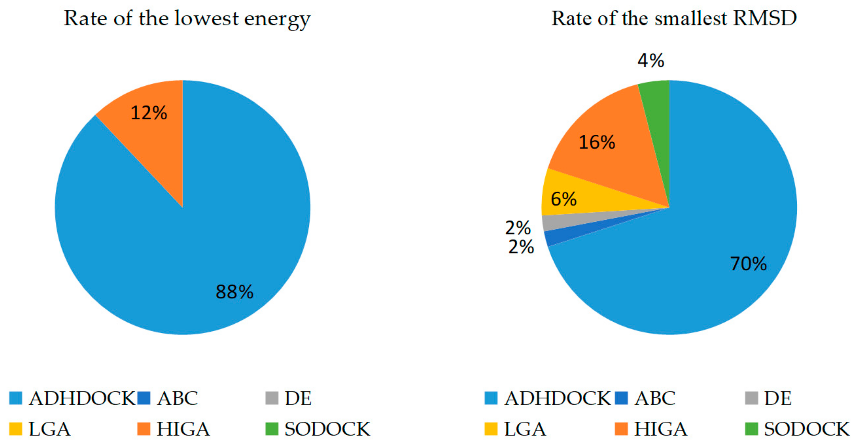
2.2. Comparison of Energy and Root-Mean-Square Deviation (RMSD)
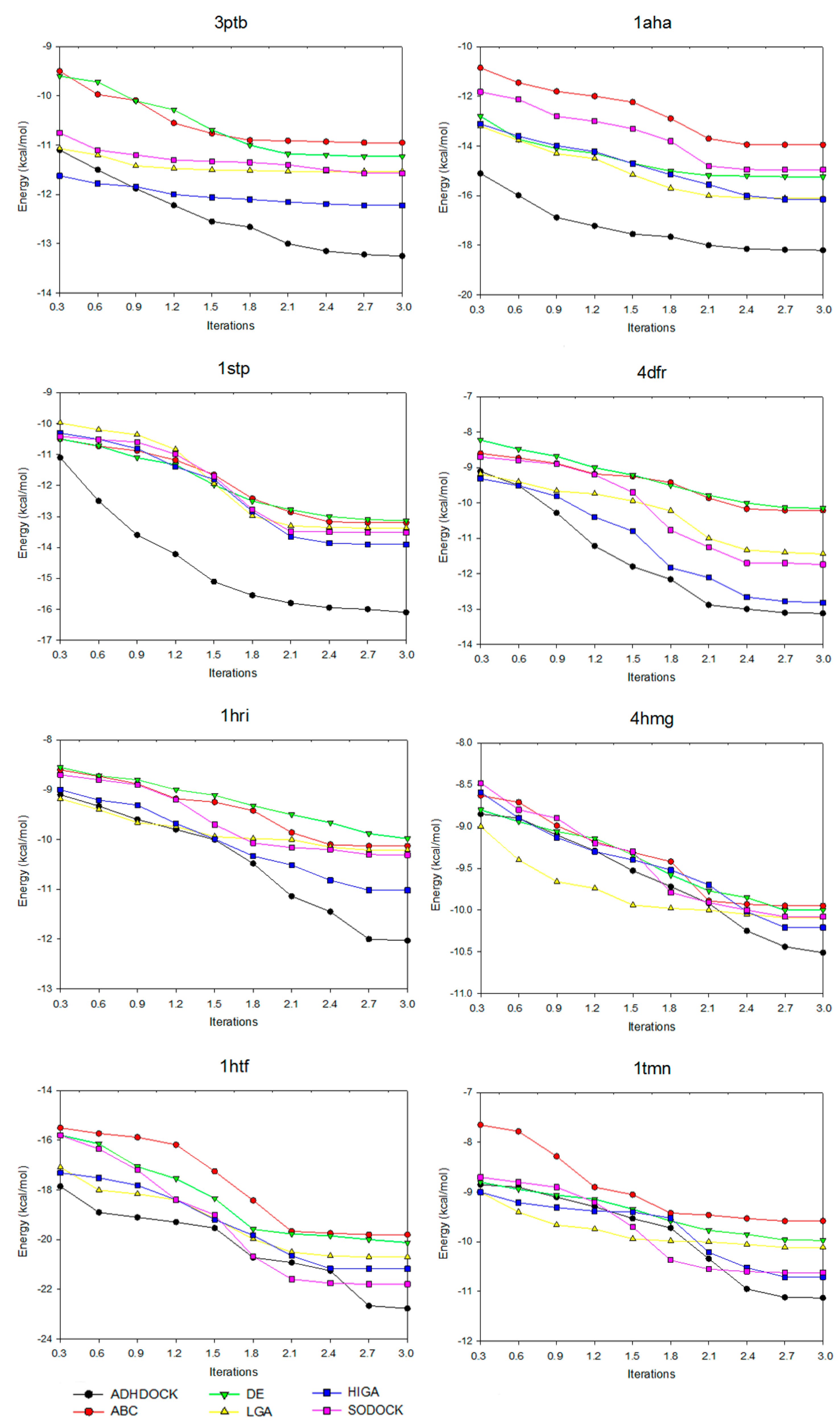
2.3. Convergence Analysis
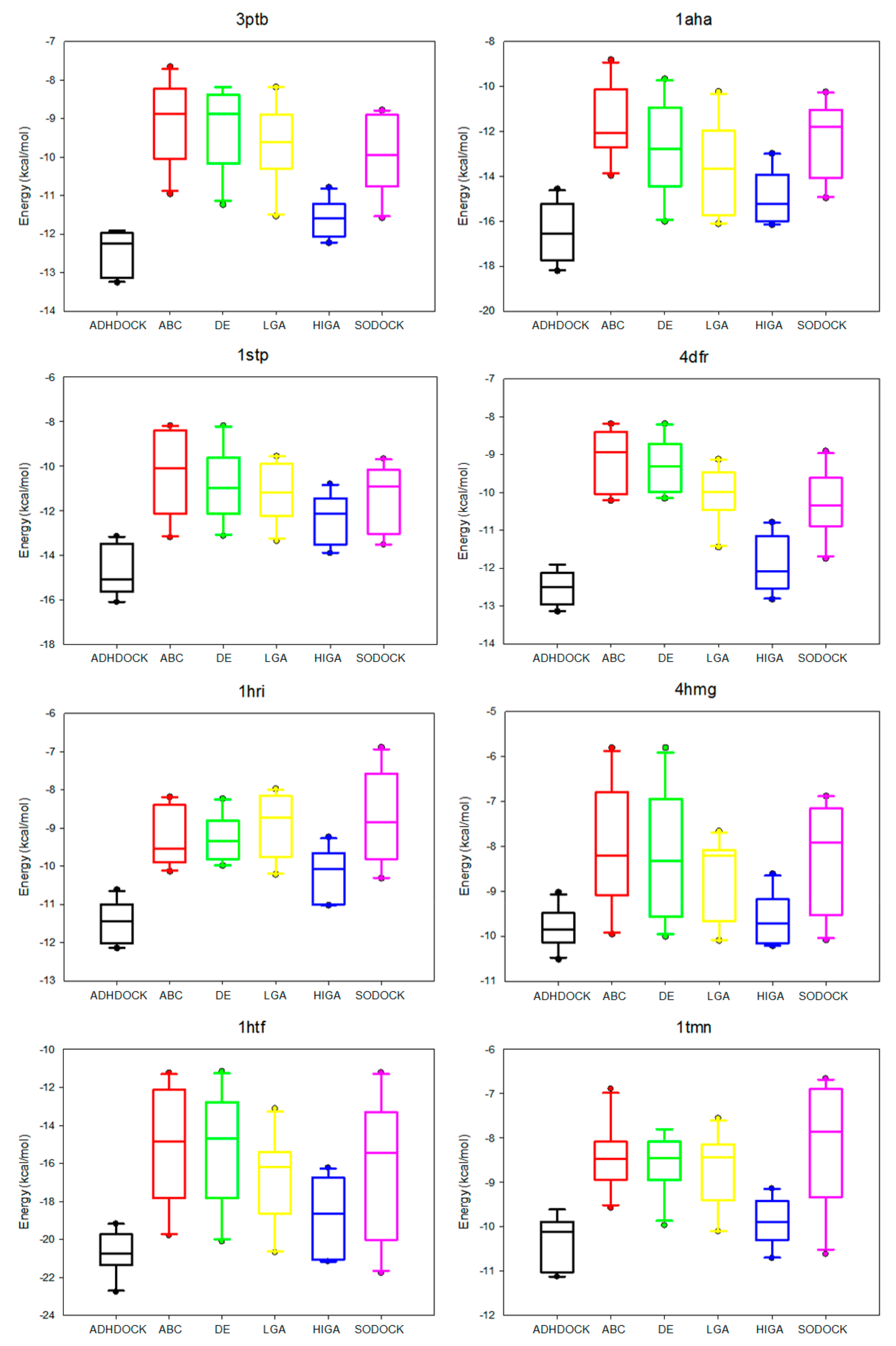
2.4. Data Distribution Analysis
2.5. Hypothesis Test
3. Discussion
4. Materials and Methods
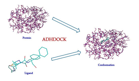
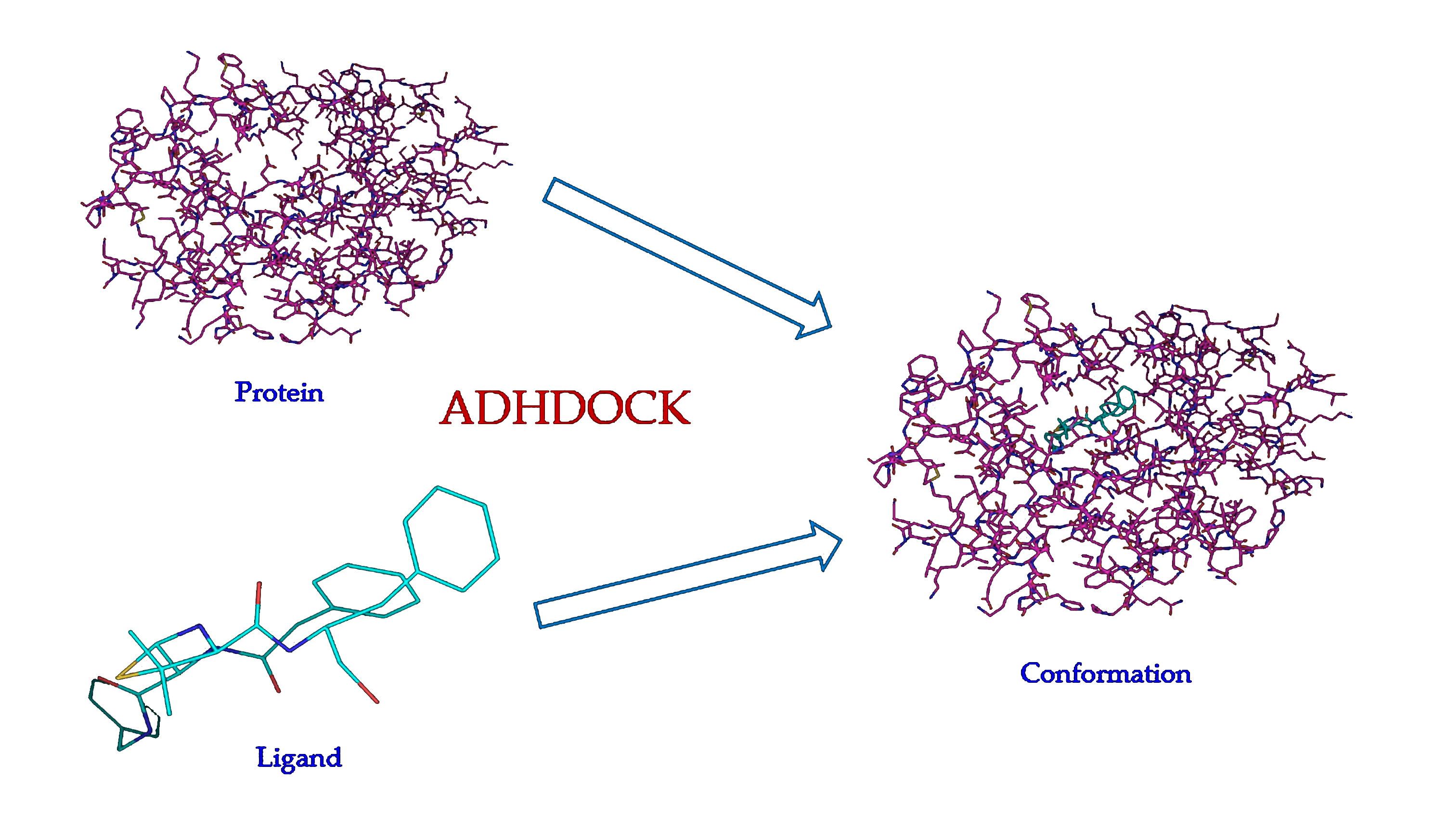
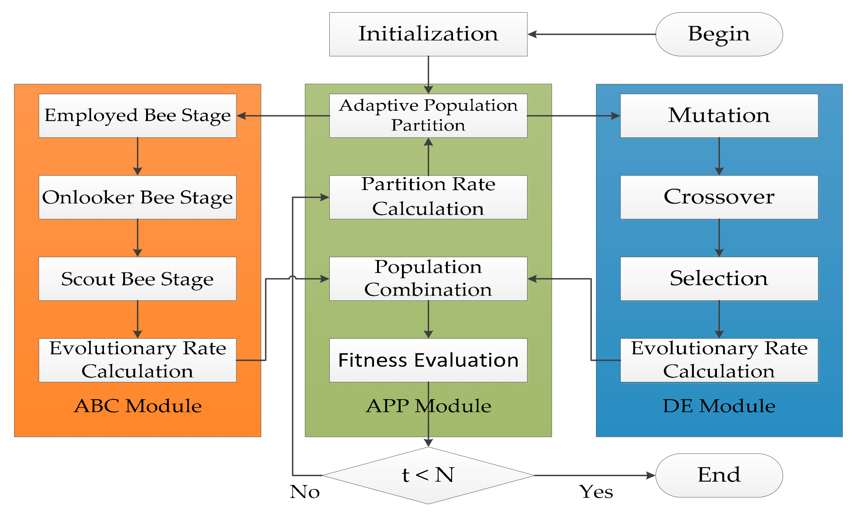
4.1. Framework of ADHDOCK
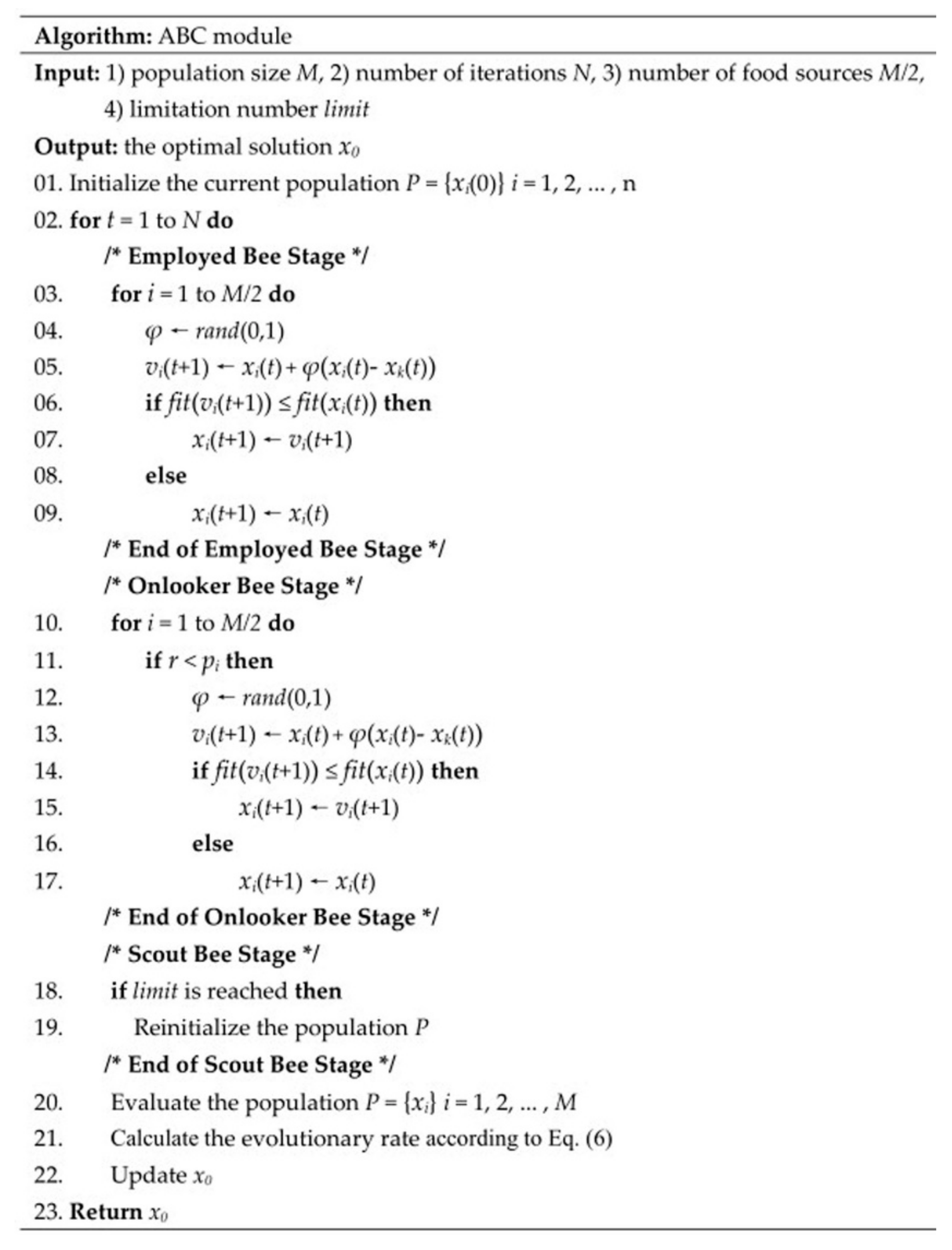
4.2. ABC Module
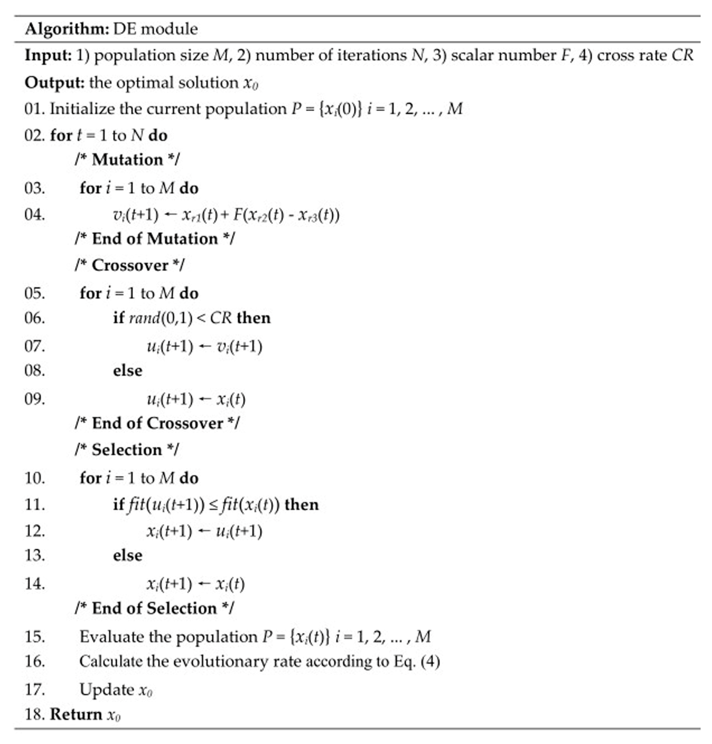
4.3. DE Module
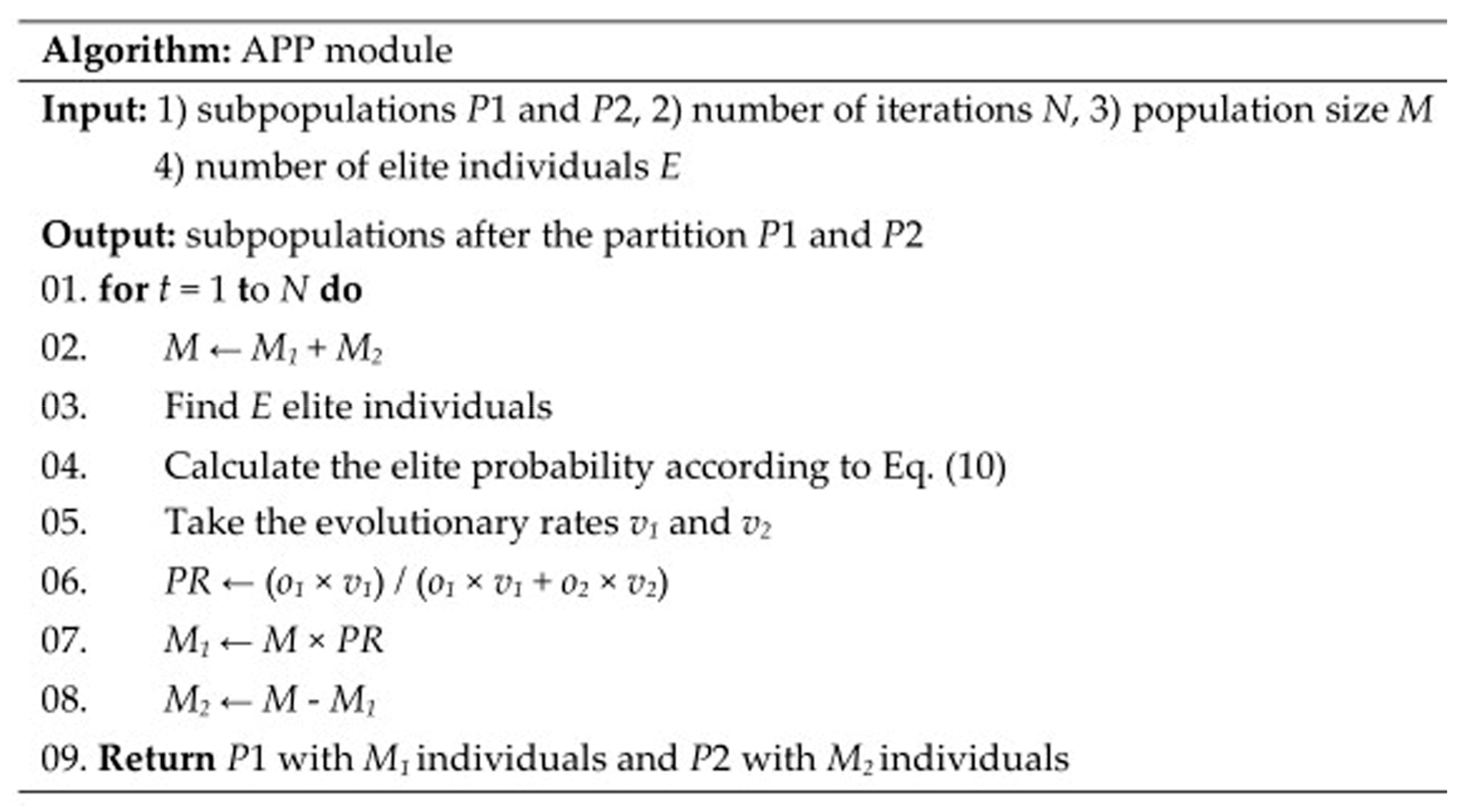
4.4. APP Module
4.5. Hybrid Search of ADHDOCK
5. Conclusions
Acknowledgments
Author Contributions
Conflicts of Interest
Abbreviations
| ADHDOCK | an efficient ABC_DE_based hybrid algorithm for protein–ligand docking |
| ABC | artificial bee colony |
| DE | differential evolution |
| HIGA | running history information guided genetic algorithm |
| PSO | particle swarm optimization |
| SODOCK | swarm optimization for highly flexible protein–ligand docking |
| APP | adaptive population partition |
| CADD | computer aided drug design |
| SA | simulated annealing |
| GA | genetic algorithm |
| LGA | Lamarckian genetic algorithm |
| RMSD | Root-mean-square deviation |
References
- Bohlooli, F.; Sepehri, S.; Razzaghi-AsI, N. Response surface methodology in drug design: A case study on docking analysis of a potent antifungal fluconazole. Comput. Biol. Chem. 2017, 67, 158–173. [Google Scholar] [CrossRef] [PubMed]
- Antón, P.R.L.; Francisco, C.; Alejandro, P.; Belén, P.P.A. Deep Artificial Neural Networks and Neuromorphic Chips for Big Data Analysis: Pharmaceutical and Bioinformatics Applications. Int. J. Mol. Sci. 2016, 17, 1313–1338. [Google Scholar]
- Allen, S.E.; Dokholyan, N.V.; Bowers, A.A. Dynamic docking of conformationally constrained macrocycles: Methods and applications. ACS Chem. Biol. 2016, 11, 10–24. [Google Scholar] [CrossRef] [PubMed]
- Zou, Q.; Li, J.J.; Song, L.; Zeng, X.X.; Wang, G.H. Similarity computation strategies in the microRNA-disease network: A Survey. Brief. Funct. Genom. 2016, 15, 55–64. [Google Scholar] [CrossRef] [PubMed]
- Bjerrum, E.J. Machine learning optimization of cross docking accuracy. Comput. Biol. Chem. 2016, 62, 133–144. [Google Scholar] [CrossRef] [PubMed]
- Guedes, I.A.; de Magalhães, C.S.; Dardenne, L.E. Receptor-ligand molecular docking. Biophys. Rev. 2014, 6, 75–87. [Google Scholar] [CrossRef] [PubMed]
- Atkovska, K.; Samsonov, S.A.; Paszkowskirogacz, M.; Pisabarro, M.T. Multipose Binding in Molecular Docking. Int. J. Mol. Sci. 2014, 15, 2622–2645. [Google Scholar] [CrossRef] [PubMed]
- Feinstein, W.P.; Brylinski, M. Calculating an optimal box size for ligand docking and virtual screening against experimental and predicted binding pockets. J. Cheminform. 2015, 7, 18. [Google Scholar] [CrossRef] [PubMed]
- Zeng, X.X.; Liao, Y.L.; Liu, Y.S.; Zou, Q. Prediction and validation of disease genes using HeteSim Scores. IEEE ACM Trans. Comput. Biol. Bioinform. 2017, 14, 687–695. [Google Scholar] [CrossRef] [PubMed]
- Zhao, Y.H.; Wang, G.R.; Zhang, X.; Yu, J.X.; Wang, Z.H. Learning Phenotype Structure Using Sequence Model. IEEE Trans. Knowl. Data Eng. 2014, 26, 667–681. [Google Scholar] [CrossRef]
- Moitessier, N.; Englebienne, P.; Lee, D.; Lawandi, J.; Gorbeil, C.R. Towards the development of universal, fast and highly accurate docking/scoring methods: A long way to go. Br. J. Pharmacol. 2008, 153, 7–26. [Google Scholar] [CrossRef] [PubMed]
- Hu, X.; Balaz, S.; Shelver, W.H. A practical approach to docking of zinc metalloproteinase inhibitors. J. Mol. Graph. Model. 2004, 22, 293–307. [Google Scholar] [CrossRef] [PubMed]
- Huey, R.; Morris, G.M.; Olson, A.J.; Goodsell, D.S. Software news and update a semiempirical free energy force field with charge−based desolvation. J. Comput. Chem. 2006, 10, 1145–1152. [Google Scholar]
- Jain, A.N. Scoring functions for protein−ligand docking. Curr. Protein Pept. Sci. 2006, 7, 407–420. [Google Scholar] [PubMed]
- Muryshev, A.E.; Tarasov, D.N.; Butygin, A.V.; Butygina, O.V.; Aleksandrov, A.B.; Nikitin, S.M. A novel scoring function for molecular docking. J. Comput. Aided Mol. Des. 2003, 17, 597–605. [Google Scholar] [CrossRef] [PubMed]
- Ain, Q.U.; Aleksandrova, A.; Roessler, F.D.; Ballester, P.J. Machine−learning scoring functions to improve structure-based binding affinity prediction and virtual screening. Wiley. Interdiscip. Rev. Comput. Mol. Sci. 2015, 5, 405–424. [Google Scholar] [CrossRef] [PubMed]
- Jug, G.; Anderluh, M.; Tomašič, T. Comparative evaluation of several docking tools for docking small molecule ligands to DC-SIGN. J. Mol. Model. 2015, 21, 164–178. [Google Scholar] [CrossRef] [PubMed]
- Castro-Alvarez, A.; Costa, A.M.; Vilarrasa, J. The Performance of Several Docking Programs at Reproducing Protein-Macrolide-Like Crystal Structures. Molecules 2017, 22, 136. [Google Scholar] [CrossRef] [PubMed]
- Guo, L.Y.; Yan, Z.Q.; Zheng, X.L.; Hu, L.; Yang, Y.L.; Wang, J. A comparison of various optimization algorithms of protein-ligand docking programs by fitness accuracy. J. Mol. Model. 2014, 20. [Google Scholar] [CrossRef] [PubMed]
- Bharatham, N.; Bharatham, K.; Shelat, A.A.; Bashford, D. Ligand binding more prediction by docking: mdm2/mdmx inhibitors as a case study. J. Chem. Inf. Model. 2014, 54, 648–659. [Google Scholar] [CrossRef] [PubMed]
- Bernauer, J.; Azé, J.; Janin, J.; Poupon, A. A new protein–protein docking scoring function based on interface residue properties. Bioinformatics 2007, 23, 555–562. [Google Scholar] [CrossRef] [PubMed]
- Li, Z.F.; Gu, J.F.; Zhuan, H.Y.; Kang, L.; Zhao, X.Y.; Guo, Q. Adaptive molecular docking method baesd on information entropy genetic algorithm. Appl. Soft Comput. 2015, 26, 299–302. [Google Scholar] [CrossRef]
- Zhao, Y.H.; Yu, J.X.; Wang, G.R.; Chen, L.; Wang, B.; Yu, G. Maximal Subspace Coregulated Gene Clustering. IEEE Trans. Knowl. Data Eng. 2008, 20, 83–98. [Google Scholar] [CrossRef]
- Blum, C.; Puchinger, J.; Raidl, G.R.; Roli, A. Hybrid mataheuristics in combinatorial optimization: A survey. Appl. Soft Comput. 2011, 11, 4135–4151. [Google Scholar] [CrossRef]
- Lόpez-Camacho, E.; Godoy, M.J.; Garcỉa-Nieto, J.; Nebro, A.J.; Aldana-Montes, J.F. Solving molecular flexible docking problems with mataheuristics: A comparative study. Appl. Soft Comput. 2015, 28, 379–393. [Google Scholar] [CrossRef]
- Thomsen, R. Flexible ligand docking using evolutionary algorithms: Investigating the effects of variation operators and local search hybrids. Biosystems 2003, 72, 57–73. [Google Scholar] [CrossRef]
- Ng, M.C.; Fong, S.; Siu, S.W. PSOVina: The hybrid particle swarm optimization algorithm for protein–ligand docking. J. Bioinform. Comput. Biol. 2015, 13. [Google Scholar] [CrossRef] [PubMed]
- Uehara, S.; Fujimoto, K.J.; Tanaka, S. Protein-ligand docking using fitness learning-based artificial bee colony with proximity stimuli. Phys. Chem. Chem. Phys. 2015, 17, 16412–16417. [Google Scholar] [CrossRef] [PubMed]
- Goodsell, D.S.; Olson, A.J. Automated docking of substrates to proteins by simulated annealing. Proteins Struct. Funct. Genet. 1990, 8, 195–202. [Google Scholar] [CrossRef] [PubMed]
- Jones, G.; Willett, P.; Glen, R.C.; Leach, A.R.; Taylor, R. Development and validation of a genetic algorithm for flexible docking. J. Mol. Biol. 1997, 267, 727–748. [Google Scholar] [CrossRef] [PubMed]
- Fuhrmann, J.; Rurainsk, A.; Lenhof, H.P.; Neumann, D. A new Lamarckian genetic algorithm for flexible ligang-receptor docking. J. Comput. Chem. 2010, 31, 1911–1918. [Google Scholar] [PubMed]
- Guan, B.; Zhang, C.; Zhao, Y. HIGA: A Running History Information Guided Genetic Algorithm for Protein–Ligand Docking. Molecules 2017, 22, 2233. [Google Scholar] [CrossRef] [PubMed]
- Chen, H.M.; Liu, B.F.; Huang, H.L.; Hwang, S.F.; Ho, S.Y. SODOCK: Swarm optimization for highly flexible protein–ligand docking. J. Comput. Chem. 2007, 28, 612–623. [Google Scholar] [CrossRef] [PubMed]
- KKaraboga, D.; Basturk, B. A powerful and efficient algorithm for numerical function optimization: Artificial bee colony (ABC) algorithm. J. Glob. Optim. 2007, 39, 459–471. [Google Scholar] [CrossRef]
- Storn, R.; Price, K. Differential Evolution—A Simple and Efficient Heuristic for global Optimization over Continuous Spaces. J. Glob. Optim. 1997, 11, 341–359. [Google Scholar] [CrossRef]
- Morris, G.M.; Huey, R.; Lindstrom, W.; Sanner, M.F.; Belew, R.K.; Goodsell, D.S.; Olson, A.J. AutoDock4 and AutoDockTools4: Automated docking with selective receptor flexibility. J. Comput. Chem. 2009, 30, 2785–2791. [Google Scholar] [CrossRef] [PubMed]
- Wang, R.X.; Fang, X.L.; Lu, Y.P.; Yang, C.Y.; Wang, S.M. The PDBbind database: Methodologies and updates. J. Med. Chem. 2005, 48, 4111–4119. [Google Scholar] [CrossRef] [PubMed]


| ADHDOCK | |
| Number of food sources | 50 |
| Number of limitation | 100 |
| Crossover rate | 0.80 |
| Scalar number | 0.90 |
| Initial partition rate | 0.50 |
| ABC | |
| Number of food sources | 50 |
| Number of limitation | 100 |
| DE | |
| Crossover rate | 0.80 |
| Scalar number | 0.90 |
| LGA | |
| Mutation rate | 0.02 |
| Crossover rate | 0.80 |
| Maximal iterations of local search | 300 |
| HIGA | |
| Mutation rate | 0.02 |
| Crossover rate | 0.80 |
| Maximal iterations of local search | 300 |
| Number of elitists | 5 |
| equilibrium factor | 0.60 |
| SODOCK | |
| Number of immediate neighbors | 4 |
| Cognitive weight | 2.00 |
| Social weight | 2.00 |
| Maximal iterations of local search | 300 |
| Algorithm | Success Case | Average RMSD (All Cases) | Average RMSD (RMSD < 2.0 Å) |
|---|---|---|---|
| ABC | 32 | 3.28 ± 1.32 | 1.84 ± 0.42 |
| DE | 35 | 3.21 ± 1.37 | 1.82 ± 0.42 |
| LGA | 34 | 2.55 ± 1.28 | 1.68 ± 0.40 |
| HIGA | 42 | 1.87 ± 0.99 | 1.36 ± 0.51 |
| SODOCK | 37 | 2.92 ± 1.08 | 1.77 ± 0.39 |
| ADHDOCK | 46 | 1.68 ± 0.89 | 1.19 ± 0.33 |
| PDB | Tor | ADHDOCK | ABC | DE | LGA | HIGA | SODOCK | ||||||
|---|---|---|---|---|---|---|---|---|---|---|---|---|---|
| Energy | RMSD | Energy | RMSD | Energy | RMSD | Energy | RMSD | Energy | RMSD | Energy | RMSD | ||
| 3ptb | 0 | −13.25 | 1.65 | −10.95 | 1.97 | −11.23 | 1.80 | −11.53 | 1.92 | −12.22 | 1.95 | −11.57 | 2.00 |
| 1hdy | 0 | −10.40 | 0.80 | −8.80 | 1.47 | −8.24 | 1.05 | −8.70 | 1.78 | −9.17 | 0.98 | −9.22 | 1.49 |
| 1aha | 1 | −18.20 | 0.82 | −13.95 | 1.85 | −15.24 | 1.22 | −16.10 | 0.45 | −16.15 | 0.90 | −14.95 | 1.44 |
| 1dbb | 1 | −12.38 | 0.35 | −11.88 | 0.88 | −11.29 | 0.55 | −11.00 | 0.72 | −11.17 | 0.80 | −11.76 | 0.88 |
| 1mrg | 1 | −8.55 | 0.30 | −7.85 | 0.85 | −7.48 | 1.25 | −6.16 | 0.40 | −7.52 | 0.33 | −8.14 | 1.20 |
| 1ulb | 1 | −7.50 | 0.72 | −5.36 | 0.80 | −5.20 | 0.40 | −6.28 | 0.74 | −7.07 | 0.35 | −6.75 | 0.50 |
| 1tnl | 2 | −9.49 | 0.36 | −5.80 | 0.68 | −6.28 | 0.52 | −6.83 | 0.73 | −8.08 | 0.62 | −6.78 | 0.88 |
| 2phh | 2 | −9.21 | 0.54 | −6.98 | 1.30 | −6.95 | 1.15 | −7.54 | 0.55 | −8.20 | 0.65 | −8.16 | 0.34 |
| 3hvt | 2 | −17.59 | 0.55 | −15.95 | 0.68 | −15.29 | 0.47 | −17.22 | 0.33 | −18.19 | 0.45 | −16.78 | 0.58 |
| 1phg | 3 | −10.28 | 0.38 | −7.95 | 1.67 | −7.90 | 1.33 | −8.56 | 0.80 | −9.58 | 0.60 | −9.15 | 1.34 |
| 2cht | 3 | −10.37 | 1.55 | −7.87 | 1.24 | −8.16 | 1.16 | −8.89 | 0.95 | −9.10 | 1.34 | −8.77 | 1.33 |
| 2ctc | 3 | −9.25 | 0.78 | −6.40 | 1.66 | −6.70 | 1.67 | −7.70 | 0.89 | −8.90 | 0.80 | −8.52 | 1.21 |
| 4cts | 3 | −9.98 | 0.55 | −6.94 | 0.95 | −6.79 | 0.68 | −7.61 | 0.75 | −8.64 | 0.48 | −9.10 | 1.20 |
| 1abe | 4 | −10.10 | 0.39 | −7.99 | 0.95 | −8.15 | 1.03 | −8.75 | 0.60 | −9.44 | 0.75 | −8.73 | 0.80 |
| 1hsl | 4 | −15.15 | 0.56 | −11.25 | 1.36 | −11.97 | 1.60 | −12.10 | 0.56 | −13.17 | 0.66 | −12.90 | 1.23 |
| 2mcp | 4 | −10.35 | 1.05 | −7.85 | 1.64 | −8.10 | 1.10 | −8.22 | 1.33 | −9.35 | 1.15 | −7.72 | 1.42 |
| 1stp | 5 | −16.10 | 0.35 | −13.20 | 1.58 | −13.13 | 0.92 | −13.37 | 1.65 | −13.90 | 0.85 | −13.52 | 1.00 |
| 1tni | 5 | −9.12 | 0.74 | −6.82 | 1.25 | −6.79 | 0.67 | −8.02 | 1.65 | −8.61 | 0.90 | −7.56 | 1.34 |
| 2lgs | 5 | −9.23 | 0.71 | −7.25 | 1.10 | −7.11 | 0.76 | −7.30 | 0.77 | −7.83 | 1.22 | −7.18 | 1.50 |
| 1acm | 6 | −11.61 | 0.30 | −9.95 | 0.33 | −9.28 | 0.40 | −10.10 | 0.37 | −10.87 | 0.33 | −10.11 | 0.45 |
| 2cgr | 6 | −18.80 | 0.70 | −14.25 | 0.97 | −14.14 | 0.80 | −16.00 | 0.76 | −17.80 | 0.75 | −15.74 | 0.77 |
| 6rnt | 6 | −9.32 | 0.55 | −8.95 | 1.45 | −8.90 | 1.65 | −9.13 | 0.70 | −9.62 | 0.50 | −9.12 | 1.95 |
| 1lst | 7 | −16.13 | 0.36 | −12.22 | 0.96 | −12.43 | 0.95 | −13.75 | 0.55 | −15.22 | 0.46 | −14.72 | 0.66 |
| 2cmd | 7 | −15.14 | 0.42 | −12.70 | 0.65 | −12.42 | 0.62 | −12.26 | 0.78 | −14.05 | 0.82 | −13.28 | 0.80 |
| 4dfr | 7 | −13.12 | 1.04 | −10.21 | 1.97 | −10.15 | 1.20 | −11.44 | 1.23 | −12.82 | 1.56 | −11.74 | 1.67 |
| 1ett | 8 | −14.90 | 1.20 | −12.75 | 1.65 | −12.40 | 1.70 | −13.89 | 1.38 | −13.94 | 1.40 | −12.08 | 1.54 |
| 1tka | 8 | −14.02 | 0.88 | −10.33 | 1.17 | −9.89 | 1.20 | −10.23 | 0.98 | −11.60 | 1.02 | −10.25 | 1.15 |
| 8gch | 8 | −14.55 | 0.70 | −10.85 | 0.82 | −11.30 | 1.15 | −11.88 | 1.72 | −12.55 | 1.66 | −11.29 | 0.98 |
| 1hri | 9 | −12.03 | 1.13 | −10.13 | 1.67 | −9.98 | 1.56 | −10.21 | 1.87 | −11.02 | 1.18 | −10.31 | 1.68 |
| 1trk | 9 | −14.50 | 0.80 | −11.25 | 0.65 | −11.35 | 0.62 | −11.44 | 0.65 | −13.05 | 0.50 | −11.49 | 0.60 |
| 2sim | 9 | −18.25 | 0.90 | −15.93 | 1.10 | −15.50 | 1.06 | −15.61 | 0.95 | −16.24 | 1.08 | −15.05 | 1.06 |
| 1eap | 10 | −14.05 | 1.25 | −12.85 | 1.21 | −12.18 | 1.30 | −13.08 | 1.27 | −14.55 | 0.98 | −13.77 | 1.10 |
| 1fkg | 10 | −17.51 | 1.13 | −15.15 | 1.20 | −15.36 | 1.22 | −15.47 | 1.36 | −16.26 | 1.35 | −15.08 | 1.38 |
| 1hvr | 10 | −33.40 | 0.55 | −28.65 | 0.85 | −29.38 | 0.78 | −30.85 | 0.62 | −31.50 | 0.80 | −29.29 | 0.68 |
| 1lna | 10 | −15.62 | 1.10 | −13.85 | 1.82 | −13.28 | 1.67 | −13.50 | 1.75 | −15.19 | 1.29 | −13.82 | 1.22 |
| 1nco | 11 | −21.70 | 0.93 | −20.54 | 0.77 | −20.85 | 0.82 | −21.20 | 0.65 | −22.75 | 0.55 | −20.60 | 0.92 |
| 4hmg | 11 | −10.51 | 1.13 | −9.95 | 1.60 | −10.00 | 1.28 | −10.09 | 1.70 | −10.21 | 1.65 | −10.08 | 1.36 |
| 1bbp | 12 | −26.90 | 0.45 | −24.48 | 0.65 | −23.38 | 0.78 | −23.56 | 0.52 | −25.10 | 0.67 | −24.15 | 0.72 |
| 1cdg | 12 | −8.95 | 1.05 | −7.13 | 1.12 | −7.72 | 1.17 | −8.22 | 1.94 | −8.90 | 1.65 | −8.45 | 1.80 |
| 1rds | 12 | −18.11 | 0.75 | −16.34 | 0.92 | −15.93 | 0.86 | −16.24 | 0.80 | −17.95 | 0.77 | −16.03 | 0.67 |
| 1htf | 13 | −22.77 | 1.02 | −19.80 | 1.80 | −20.12 | 1.48 | −20.69 | 1.33 | −21.17 | 1.20 | −21.79 | 1.42 |
| 1glq | 14 | −9.83 | 1.15 | −9.23 | 1.58 | −8.53 | 1.29 | −9.27 | 1.87 | −9.65 | 1.25 | −8.83 | 1.90 |
| 1hpv | 14 | −16.72 | 1.96 | −15.67 | 1.91 | −15.11 | 1.92 | −15.48 | 1.88 | −17.29 | 1.60 | −15.68 | 1.75 |
| 1qbt | 14 | −26.75 | 0.80 | −22.69 | 1.29 | −22.93 | 1.27 | −24.20 | 1.09 | −25.20 | 0.88 | −24.63 | 1.04 |
| 1lic | 15 | −12.77 | 0.85 | −10.01 | 1.36 | −9.80 | 1.54 | −12.17 | 1.80 | −13.03 | 0.96 | −12.55 | 1.08 |
| 1tmn | 15 | −11.13 | 0.90 | −9.58 | 0.65 | −9.97 | 1.18 | −10.11 | 1.20 | −10.71 | 0.95 | −10.62 | 1.95 |
| 4phv | 15 | −22.44 | 1.38 | −15.62 | 1.44 | −16.08 | 1.53 | −19.18 | 1.26 | −19.89 | 0.45 | −21.78 | 0.90 |
| 1epo | 17 | −20.33 | 0.80 | −16.07 | 1.77 | −17.18 | 1.62 | −16.80 | 1.67 | −19.13 | 1.23 | −17.65 | 0.93 |
| 1aaq | 20 | −23.10 | 1.10 | −15.55 | 1.20 | −16.60 | 1.75 | −17.44 | 1.70 | −20.66 | 1.05 | −19.80 | 1.34 |
| 1hiv | 23 | −25.60 | 0.55 | −15.45 | 1.06 | −16.20 | 0.73 | −17.95 | 1.73 | −21.25 | 1.21 | −19.74 | 1.55 |
| PDB | ABC | DE | LGA | HIGA | SODOCK |
|---|---|---|---|---|---|
| 3ptb | 4.49 × 10⁻⁸ | 3.17 × 10⁻⁴ | 2.15 × 10⁻³ | 7.12 × 10⁻³ | 3.32 × 10⁻⁴ |
| 1hdy | 1.18 × 10⁻⁴ | 2.39 × 10⁻⁹ | 3.04 × 10⁻⁶ | 2.50 × 10⁻³ | 1.02 × 10⁻³ |
| 1aha | 6.41 × 10⁻¹¹ | 4.13 × 10⁻⁷ | 5.14 × 10⁻⁵ | 3.76 × 10⁻⁴ | 4.31 × 10⁻¹⁰ |
| 1dbb | 2.27 × 10⁻³ | 1.03 × 10⁻³ | 4.15 × 10⁻⁴ | 3.25 × 10⁻⁴ | 1.43 × 10⁻³ |
| 1mrg | 2.19 × 10⁻⁴ | 6.37 × 10⁻⁵ | 2.43 × 10⁻⁸ | 4.57 × 10⁻⁴ | 1.42 × 10⁻¹ |
| 1ulb | 3.91 × 10⁻⁷ | 2.31 × 10⁻⁸ | 8.15 × 10⁻⁴ | 4.35 × 10⁻³ | 2.82 × 10⁻⁴ |
| 1tnl | 4.93 × 10⁻¹⁰ | 3.86 × 10⁻⁹ | 2.62 × 10⁻⁸ | 2.14 × 10⁻⁵ | 5.90 × 10⁻⁸ |
| 2phh | 1.76 × 10⁻⁵ | 2.59 × 10⁻⁵ | 3.98 × 10⁻⁴ | 1.45 × 10⁻³ | 2.08 × 10⁻³ |
| 3hvt | 8.99 × 10⁻⁶ | 7.34 × 10⁻⁷ | 4.12 × 10⁻² | 9.98 × 10⁻¹ | 3.06 × 10⁻⁸ |
| 1phg | 3.77 × 10⁻⁶ | 6.33 × 10⁻⁶ | 3.37 × 10⁻⁴ | 1.51 × 10⁻¹ | 9.12 × 10⁻² |
| 2cht | 1.74 × 10⁻⁸ | 2.78 × 10⁻⁷ | 4.09 × 10⁻⁵ | 2.74 × 10⁻⁴ | 6.32 × 10⁻⁵ |
| 2ctc | 4.86 × 10⁻⁸ | 3.96 × 10⁻⁸ | 9.25 × 10⁻⁴ | 7.46 × 10⁻³ | 3.74 × 10⁻⁴ |
| 4cts | 3.14 × 10⁻⁸ | 1.19 × 10⁻⁹ | 3.82 × 10⁻⁶ | 2.39 × 10⁻⁴ | 7.22 × 10⁻³ |
| 1abe | 3.38 × 10⁻¹² | 4.31 × 10⁻¹⁰ | 2.35 × 10⁻⁶ | 3.55 × 10⁻³ | 2.04 × 10⁻⁶ |
| 1hsl | 1.19 × 10⁻¹⁰ | 3.08 × 10⁻⁸ | 1.05 × 10⁻⁶ | 5.32 × 10⁻⁴ | 3.91 × 10⁻⁵ |
| 2mcp | 4.15 × 10⁻⁹ | 9.30 × 10⁻⁶ | 3.21 × 10⁻⁶ | 2.86 × 10⁻⁴ | 8.82 × 10⁻⁹ |
| 1stp | 2.42 × 10⁻⁷ | 1.11 × 10⁻⁷ | 8.25 × 10⁻⁶ | 3.32 × 10⁻⁵ | 3.45 × 10⁻⁶ |
| 1tni | 3.14 × 10⁻⁸ | 1.43 × 10⁻⁸ | 3.71 × 10⁻⁵ | 8.46 × 10⁻³ | 1.58 × 10⁻⁵ |
| 2lgs | 2.37 × 10⁻⁵ | 1.33 × 10⁻⁹ | 2.54 × 10⁻⁸ | 4.52 × 10⁻⁵ | 2.28 × 10⁻⁴ |
| 1acm | 1.42 × 10⁻⁸ | 2.12 × 10⁻⁹ | 5.18 × 10⁻⁴ | 3.15 × 10⁻² | 4.12 × 10⁻⁴ |
| 2cgr | 3.39 × 10⁻⁷ | 1.07 × 10⁻⁹ | 3.95 × 10⁻⁴ | 2.14 × 10⁻² | 7.38 × 10⁻⁴ |
| 6rnt | 3.51 × 10⁻⁴ | 4.52 × 10⁻⁴ | 2.49 × 10⁻¹ | 9.82 × 10⁻¹ | 1.01 × 10⁻¹ |
| 1lst | 1.78 × 10⁻¹⁰ | 2.91 × 10⁻⁸ | 3.53 × 10⁻⁵ | 5.54 × 10⁻³ | 2.32 × 10⁻⁴ |
| 2cmd | 4.58 × 10⁻⁷ | 9.12 × 10⁻⁷ | 2.38 × 10⁻⁸ | 1.13 × 10⁻³ | 3.35 × 10⁻⁵ |
| 4dfr | 1.26 × 10⁻⁸ | 1.09 × 10⁻⁹ | 7.74 × 10⁻⁴ | 2.52 × 10⁻³ | 1.34 × 10⁻⁴ |
| 1ett | 2.29 × 10⁻⁶ | 8.17 × 10⁻⁷ | 1.16 × 10⁻⁴ | 7.70 × 10⁻³ | 1.02 × 10⁻⁸ |
| 1tka | 4.75 × 10⁻⁸ | 3.92 × 10⁻¹⁰ | 2.97 × 10⁻⁷ | 3.63 × 10⁻⁵ | 2.18 × 10⁻⁷ |
| 8gch | 2.48 × 10⁻⁶ | 8.19 × 10⁻⁵ | 4.08 × 10⁻⁵ | 1.40 × 10⁻⁴ | 9.03 × 10⁻⁵ |
| 1hri | 4.12 × 10⁻⁴ | 3.88 × 10⁻⁵ | 6.11 × 10⁻² | 2.54 × 10⁻¹ | 8.42 × 10⁻² |
| 1trk | 1.61 × 10⁻⁸ | 5.30 × 10⁻⁷ | 3.76 × 10⁻⁷ | 2.96 × 10⁻³ | 1.18 × 10⁻⁷ |
| 2sim | 3.29 × 10⁻⁵ | 3.97 × 10⁻⁵ | 1.05 × 10⁻⁶ | 4.52 × 10⁻² | 7.12 × 10⁻⁶ |
| 1eap | 1.54 × 10⁻⁴ | 2.98 × 10⁻⁶ | 3.67 × 10⁻³ | 8.56 × 10⁻¹ | 1.52 × 10⁻¹ |
| 1fkg | 4.92 × 10⁻⁵ | 3.73 × 10⁻⁵ | 9.13 × 10⁻⁴ | 1.19 × 10⁻⁴ | 9.62 × 10⁻⁶ |
| 1hvr | 1.01 × 10⁻⁷ | 2.92 × 10⁻⁵ | 1.93 × 10⁻⁴ | 8.52 × 10⁻³ | 8.32 × 10⁻⁵ |
| 1lna | 2.29 × 10⁻⁵ | 5.37 × 10⁻⁶ | 9.10 × 10⁻⁵ | 6.13 × 10⁻³ | 3.40 × 10⁻⁵ |
| 1nco | 1.02 × 10⁻² | 6.13 × 10⁻² | 2.24 × 10⁻¹ | 8.12 × 10⁻¹ | 5.46 × 10⁻² |
| 4hmg | 6.15 × 10⁻⁶ | 2.23 × 10⁻⁵ | 8.75 × 10⁻⁴ | 1.40 × 10⁻⁴ | 1.07 × 10⁻⁵ |
| 1bbp | 1.07 × 10⁻⁵ | 8.13 × 10⁻⁷ | 2.82 × 10⁻⁷ | 4.94 × 10⁻³ | 2.85 × 10⁻⁵ |
| 1cdg | 8.32 × 10⁻⁶ | 1.02 × 10⁻⁶ | 7.21 × 10⁻⁴ | 7.16 × 10⁻² | 1.14 × 10⁻⁴ |
| 1rds | 3.91 × 10⁻⁴ | 4.27 × 10⁻⁷ | 6.15 × 10⁻⁴ | 6.26 × 10⁻² | 1.08 × 10⁻⁵ |
| 1htf | 2.24 × 10⁻⁷ | 6.27 × 10⁻⁶ | 1.80 × 10⁻⁶ | 3.42 × 10⁻⁴ | 1.17 × 10⁻⁴ |
| 1glq | 7.59 × 10⁻⁵ | 8.18 × 10⁻⁸ | 2.60 × 10⁻⁵ | 1.51 × 10⁻⁴ | 3.58 × 10⁻⁷ |
| 1hpv | 7.12 × 10⁻² | 3.92 × 10⁻⁴ | 6.15 × 10⁻² | 8.15 × 10⁻¹ | 9.33 × 10⁻² |
| 1qbt | 8.04 × 10⁻⁹ | 2.71 × 10⁻⁹ | 1.16 × 10⁻⁶ | 2.12 × 10⁻⁴ | 5.72 × 10⁻⁴ |
| 1lic | 2.43 × 10⁻⁷ | 6.39 × 10⁻⁷ | 8.18 × 10⁻³ | 6.88 × 10⁻¹ | 5.89 × 10⁻² |
| 1tmn | 2.06 × 10⁻⁷ | 6.18 × 10⁻⁷ | 2.93 × 10⁻⁶ | 3.52 × 10⁻⁴ | 9.86 × 10⁻⁴ |
| 4phv | 1.35 × 10⁻¹¹ | 5.13 × 10⁻⁹ | 4.75 × 10⁻⁶ | 6.56 × 10⁻⁶ | 1.12 × 10⁻⁴ |
| 1epo | 7.87 × 10⁻¹⁰ | 1.03 × 10⁻⁶ | 3.42 × 10⁻⁸ | 1.04 × 10⁻³ | 2.77 × 10⁻⁶ |
| 1aaq | 1.02 × 10⁻¹⁰ | 5.52 × 10⁻⁸ | 1.24 × 10⁻⁷ | 3.18 × 10⁻⁵ | 6.19 × 10⁻⁷ |
| 1hiv | 8.91 × 10⁻⁹ | 4.43 × 10⁻⁸ | 6.88 × 10⁻⁷ | 2.86 × 10⁻⁴ | 1.58 × 10⁻⁶ |
© 2018 by the authors. Licensee MDPI, Basel, Switzerland. This article is an open access article distributed under the terms and conditions of the Creative Commons Attribution (CC BY) license (http://creativecommons.org/licenses/by/4.0/).
Share and Cite
Guan, B.; Zhang, C.; Zhao, Y. An Efficient ABC_DE_Based Hybrid Algorithm for Protein–Ligand Docking. Int. J. Mol. Sci. 2018, 19, 1181. https://doi.org/10.3390/ijms19041181
Guan B, Zhang C, Zhao Y. An Efficient ABC_DE_Based Hybrid Algorithm for Protein–Ligand Docking. International Journal of Molecular Sciences. 2018; 19(4):1181. https://doi.org/10.3390/ijms19041181
Chicago/Turabian StyleGuan, Boxin, Changsheng Zhang, and Yuhai Zhao. 2018. "An Efficient ABC_DE_Based Hybrid Algorithm for Protein–Ligand Docking" International Journal of Molecular Sciences 19, no. 4: 1181. https://doi.org/10.3390/ijms19041181
APA StyleGuan, B., Zhang, C., & Zhao, Y. (2018). An Efficient ABC_DE_Based Hybrid Algorithm for Protein–Ligand Docking. International Journal of Molecular Sciences, 19(4), 1181. https://doi.org/10.3390/ijms19041181