
Accurate Ab Initio and Template-Based Prediction of Short Intrinsically-Disordered Regions by Bidirectional Recurrent Neural Networks Trained on Large-Scale Datasets

Abstract
:1. Introduction
2. Results and Discussion

| Predictor | Sens | Spec | Prec | Acc | MCC |
|---|---|---|---|---|---|
| MSA | 0.867 | 0.847 | 0.268 | 0.857 | 0.430 |
| MSA-SS-SA | 0.534 | 0.983 | 0.671 | 0.732 | 0.568 |
| MSA-Templ | 0.584 | 0.983 | 0.692 | 0.783 | 0.615 |
| MSA-SS-SA-Templ | 0.606 | 0.982 | 0.684 | 0.794 | 0.622 |
| NN | 0.698 | 0.877 | 0.220 | 0.632 | 0.377 |

| Predictor | Sens | Spec | Prec | Acc | MCC |
|---|---|---|---|---|---|
| MSA | 0.818 | 0.871 | 0.284 | 0.845 | 0.432 |
| MSA-SS-SA | 0.535 | 0.982 | 0.657 | 0.738 | 0.570 |
| MSA-Templ | 0.582 | 0.982 | 0.676 | 0.782 | 0.605 |
| MSA-SS-SA-Templ | 0.603 | 0.981 | 0.672 | 0.792 | 0.615 |
| NN | 0.693 | 0.847 | 0.218 | 0.628 | 0.372 |
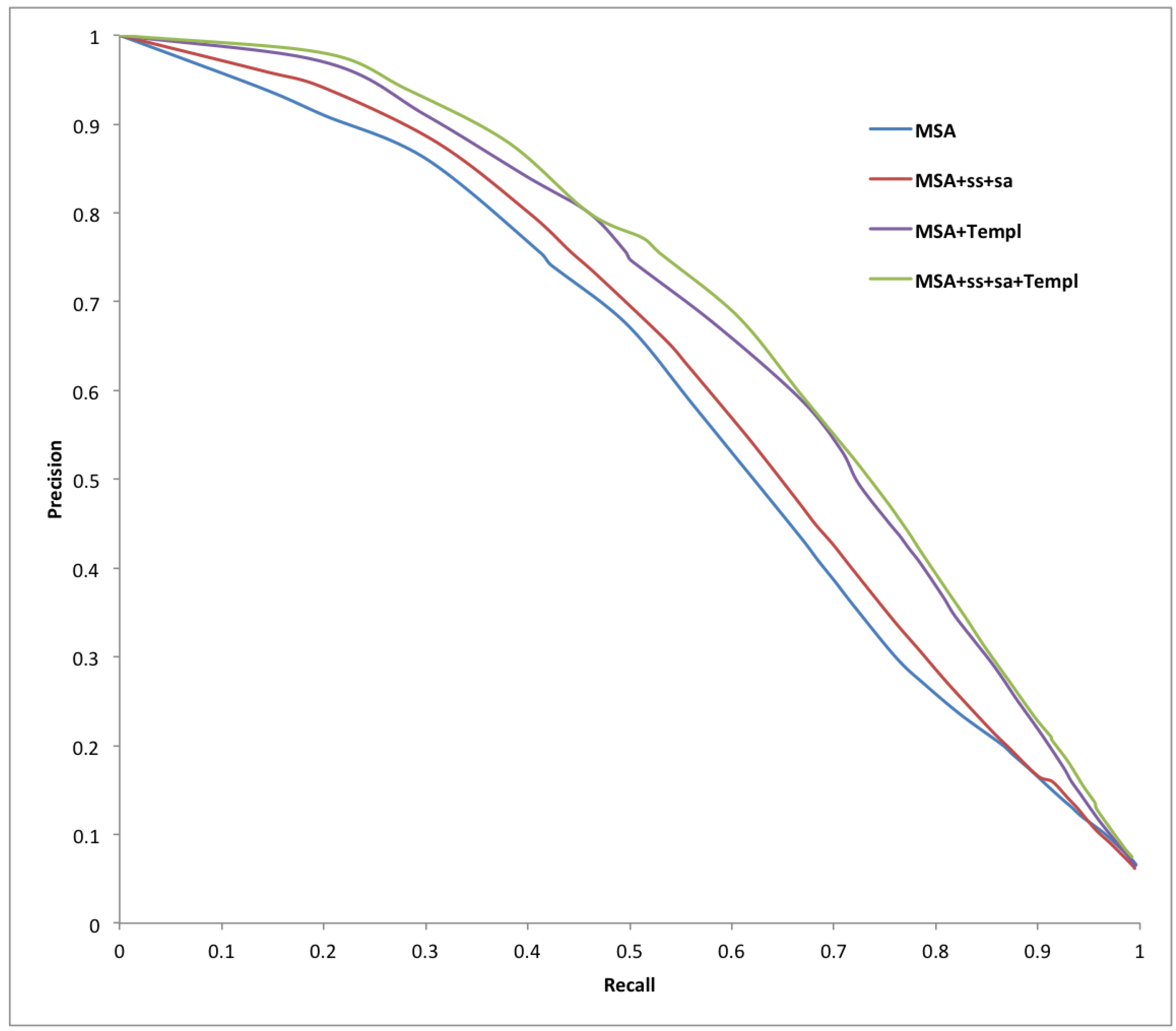
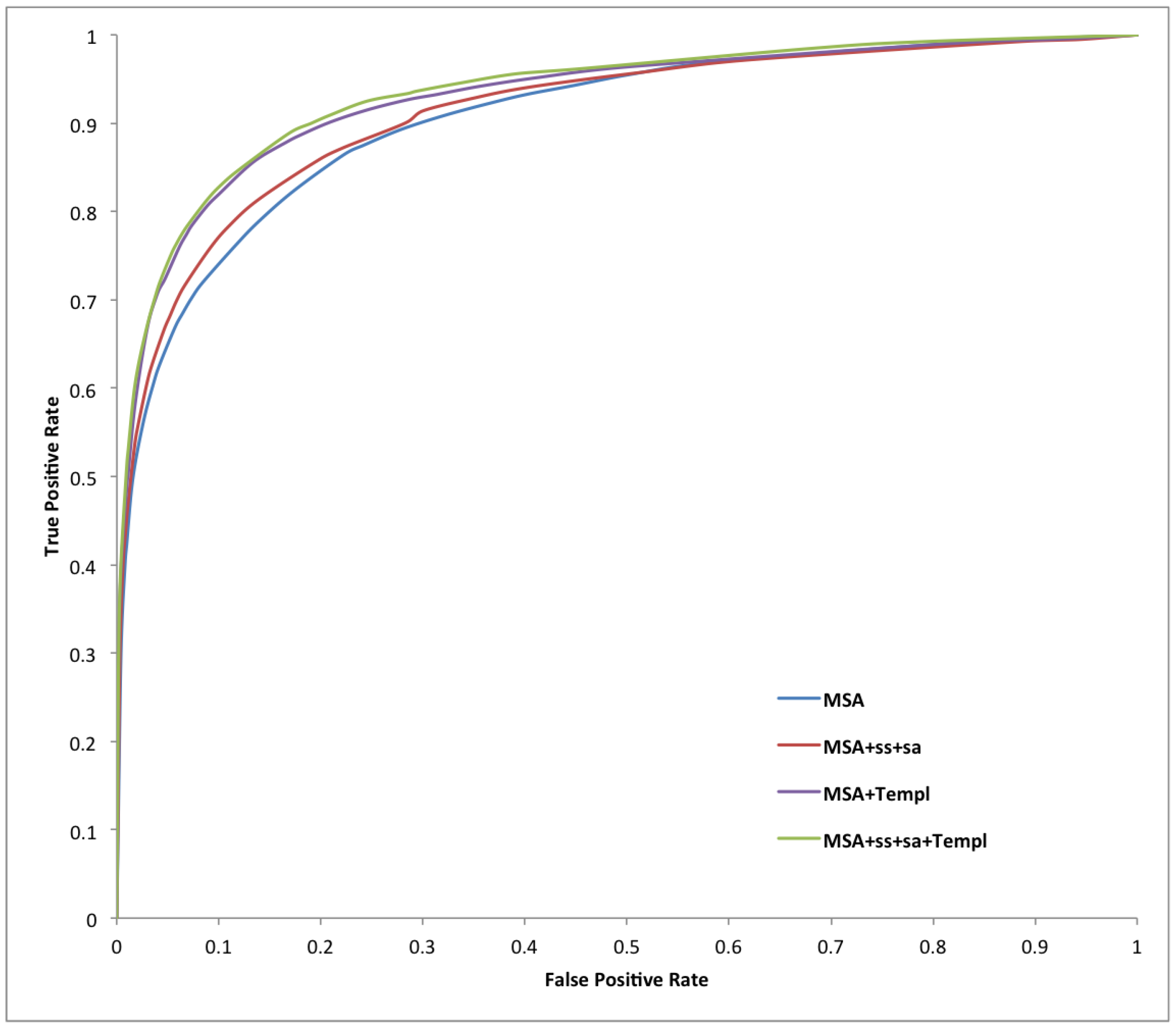
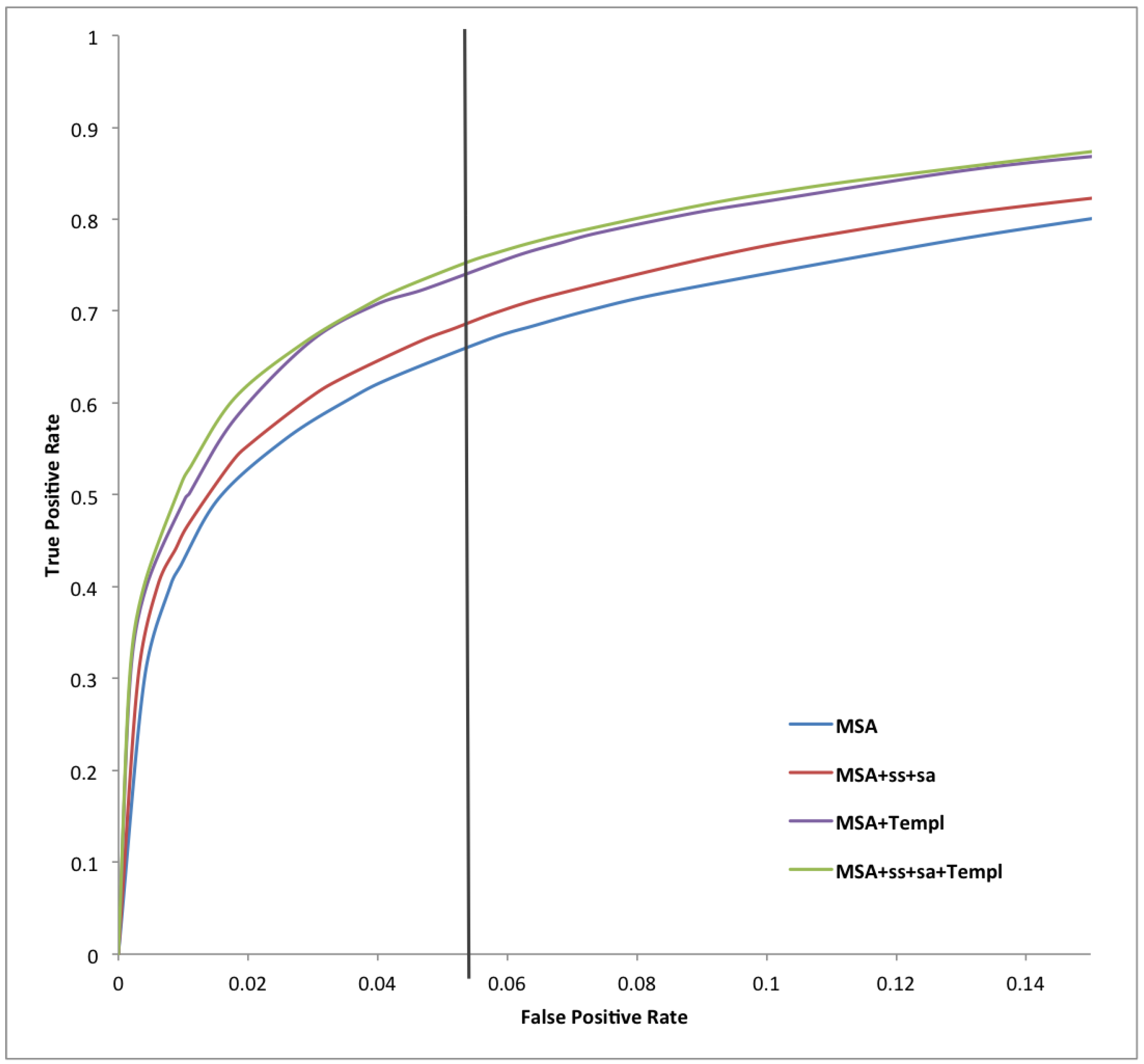
| Predictor | AUC_ROC | AUC_PR |
|---|---|---|
| MSA | 0.919 | 0.634 |
| MSA-SS-SA | 0.913 | 0.614 |
| MSA-Templ | 0.920 | 0.658 |
| MSA-SS-SA-Templ | 0.925 | 0.661 |
| NN | 0.914 | 0.617 |
3. Experimental Section
3.1. Bidirectional Recurrent Neural Networks
3.2. Input Encoding
| System | Input Component | ||||
|---|---|---|---|---|---|
| e | s | a | t | Total | |
| MSA | 21 | 0 | 0 | 0 | 21 |
| MSA-SS-SA | 21 | 3 | 4 | 0 | 28 |
| MSA-Templ | 21 | 0 | 0 | 3 | 24 |
| MSA-SS-SA-Templ | 21 | 3 | 4 | 3 | 31 |
4. Training/Testing Datasets
4.1. Training Protocol, Ensembling
4.2. Measuring Performances
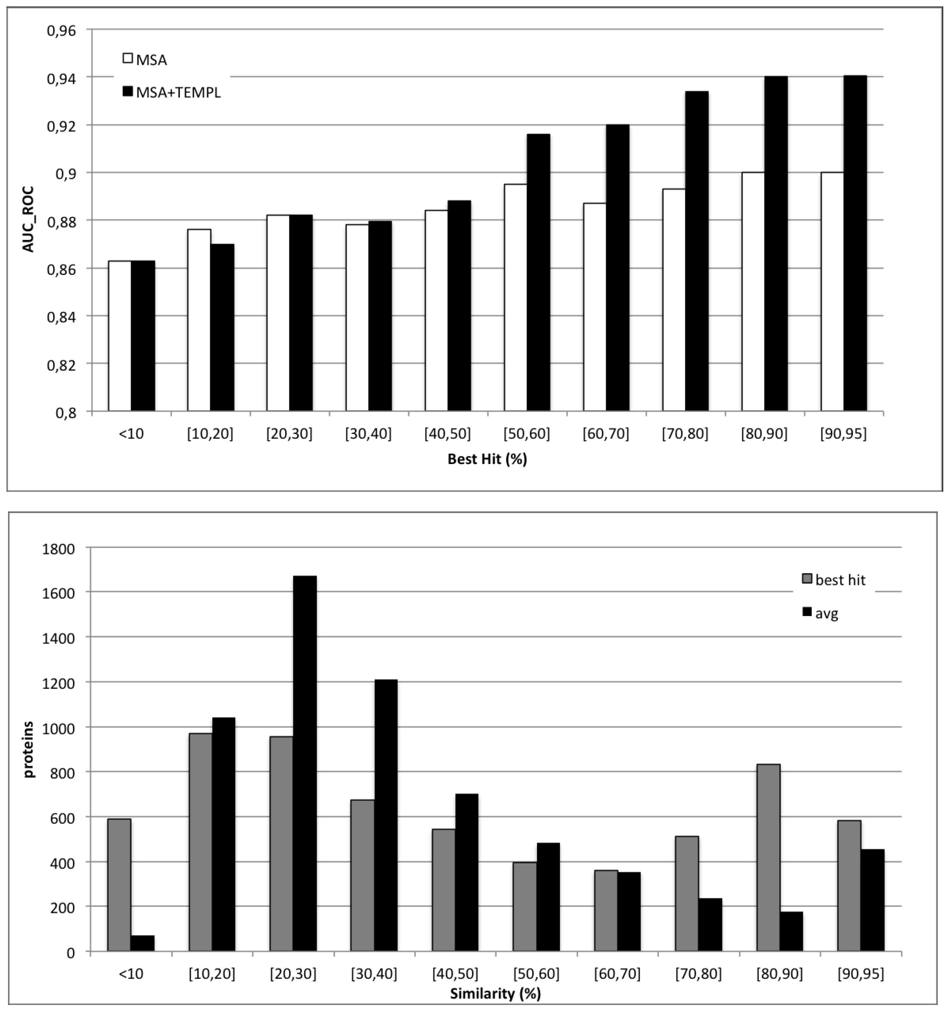
4.3. Applicability of Templates
4.4. CASP10 Results

| Predictor | Sen | Spec | AUC_ROC |
|---|---|---|---|
| MSA-SS-SA-Templ | 0.603 | 0.981 | 0.925 |
| MSA-Templ | 0.582 | 0.982 | 0.920 |
| MSA-SS-SA | 0.535 | 0.982 | 0.913 |
| MSA | 0.818 | 0.871 | 0.919 |
| CSpritz | 0.796 | 0.850 | 0.899 |
| ESpritz | 0.773 | 0.856 | 0.891 |
| SSpritzP | 0.765 | 0.870 | 0.889 |
| ESpritzP | 0.775 | 0.853 | 0.888 |
| MULTICOM | 0.820 | 0.804 | 0.888 |
| PONDR-FIT | 0.692 | 0.867 | 0.861 |
| IUPred(short) | 0.540 | 0.949 | 0.847 |
| Disopred | 0.565 | 0.939 | 0.839 |
| Predictor | MCC | AUC_ROC |
|---|---|---|
| MSA-SS-SA + templ95_94_internal | 0.480 | 0.873 |
| MSA-SS-SA + templ95_85_internal | 0.476 | 0.869 |
| MSA-templ95_94_internal | 0.434 | 0.865 |
| MSA-templ95_85_internal | 0.426 | 0860 |
| MSA-SS-SA + templ50_85_internal | 0.405 | 0.851 |
| DISOPRED3 | 0.405 | 0.850 |
| MSA-SS-SA + templ50_94_internal | 0.400 | 0.857 |
| MSA-SS-SA_94 | 0.393 | 0.845 |
| MSA-SS-SA_85 | 0.389 | 0.840 |
| MSA_94 | 0.377 | 0.831 |
| Prods-CNF | 0.375 | 0.865 |
| Biomine_dr_mixed | 0.370 | 0.850 |
| MSA_85 | 0.368 | 0.821 |
| MSA-templ50_94_internal | 0.345 | 0.833 |
| MSA-templ50_85_internal | 0.334 | 0.831 |
| DisMeta | 0.325 | 0.625 |
| Biomine_dr_pdb_c | 0.315 | 0.850 |
5. Conclusions
Acknowledgements
Author Contributions
Conflicts of Interest
References
- Habchi, J.; Tompa, P.; Longhi, S.; Uversky, V.N. Introducing protein intrinsic disorder. Chem. Rev. 2014. [Google Scholar] [CrossRef] [PubMed]
- Wright, P.; Dyson, H. Intrinsically unstructured proteins: Re-assessing the protein structure-function paradigm. J. Mol. Biol. 1999, 293, 321–331. [Google Scholar] [CrossRef] [PubMed]
- Dunker, A.; Obradovic, Z. The protein trinity-linking function and disorder. Nat. Biotechnol. 2001, 19, 805–806. [Google Scholar] [CrossRef] [PubMed]
- Tompa, P. Intrinsically unstructured proteins. Trends. Biochem. Sci. 2002, 27, 523–533. [Google Scholar] [CrossRef]
- Wright, P.E.; Dyson, H.J. Intrinsically disordered proteins in cellular signalling and regulation. Nat. Rev. Mol. Cell Biol. 2015, 16, 18. [Google Scholar] [CrossRef] [PubMed]
- Radivojac, P.; Obradovic, Z.; Smith, D.; Zhu, G.; Vucetic, S.; Brown, C.J.; Lawson, J.D.; Dunker, A.K. Protein flexibility and intrinsic disorder. Protein Sci. 2004, 13, 71–80. [Google Scholar] [CrossRef] [PubMed]
- Dunker, A.; Silman, I.; Uversky, V.; Sussman, J. Function and structure of inherently disordered proteins. Curr. Opin. Struct. Biol. 2008, 18, 756–764. [Google Scholar] [CrossRef] [PubMed]
- Oldfield, C.J.; Dunker, A.K. Intrinsically disordered proteins and intrinsically disordered protein regions. Annu. Rev. Biochem. 2014, 83, 553–584. [Google Scholar] [CrossRef] [PubMed]
- Dyson, H.; Wright, P. Coupling of folding and binding for unstructured proteins. Curr. Opin. Struct. Biol. 2002, 12, 54–60. [Google Scholar] [CrossRef]
- He, B.; Wang, K.; Liu, Y.; Xue, B.; Uversky, V.; Dunker, A. Coupling of folding and binding for unstructured proteins. Cell Res. 2009, 19, 929–949. [Google Scholar] [CrossRef] [PubMed]
- Dunker, A.; Garner, E.; Guilliot, S.; Romero, P.; Albrecht, K. Protein disorder and the evolution of molecular recognition theory predictions and observations. Pac. Symp. Biocomput. 1998, 473–484. [Google Scholar]
- Russell, R.; Gibson, T. A careful disorderliness in the proteome: Sites for interaction and targets for future therapies. FEBS Lett. 2008, 582, 1271–1275. [Google Scholar] [CrossRef] [PubMed]
- Tompa, P.; Csermely, P. The role of structural disorder in the function of RNA and protein chaperones. FASEB J. 2004, 18, 1169–1175. [Google Scholar] [CrossRef] [PubMed]
- Romero, P.R.; Zaidi, S.; Fang, Y.; Uversky, V.N.; Radivojac, P.; Oldfield, C.J.; Cortese, M.S.; Sickmeier, M.; LeGall, T.; Obradovic, Z.; et al. Alternative splicing in concert with protein intrinsic disorder enables increased functional diversity in multicellular organisms. Proc. Natl. Acad. Sci. USA 2006, 103, 8390–8395. [Google Scholar] [CrossRef] [PubMed]
- Lee, D.; Redfern, O.; Orengo, C. Predicting protein function from sequence and structure. Nat. Rev. Mol. Cell Biol. 2007, 8, 995. [Google Scholar] [CrossRef] [PubMed]
- Dunker, A.; Brown, C.; Lawson, J.; Iakoucheva, L.; Obradovic, Z. Intrinsic disorder and protein function. Biochemistry 2002, 41, 6573–6582. [Google Scholar] [CrossRef] [PubMed]
- Uversky, V.; Oldfield, C.; Dunker, A. Intrinsically disordered proteins in human diseases: Introducing the D2 concept. Annu. Rev. Biophys. 2008, 37, 215–246. [Google Scholar] [CrossRef] [PubMed]
- Peng, K.; Radivojac, P.; Vucetic, S.; Dunker, A.K.; Obradovic, Z. Length-dependent prediction of protein intrinsic disorder. BMC Bioinform. 2006, 7, 208. [Google Scholar] [CrossRef] [PubMed]
- Lobley, A.; Swindells, M.; Orengo, C.; Jones, D. Inferring function using patterns of native disorder in proteins. PLoS Comput. Biol. 2007, 3, e162. [Google Scholar] [CrossRef] [PubMed]
- Jensen, L.J.; Gupta, R.; Blom, N.; Devos, D.; Tamames, J.; Kesmir, C.; Nielsen, H.; Stærfeldt, H.H.; Rapacki, K.; Workman, C.; et al. Prediction of human protein function form post-translational modifications and localization features. J. Mol. Biol. 2002, 319, 1257–1265. [Google Scholar] [CrossRef]
- Schlessinger, A.; Schaefer, C.; Vicedo, E.; Schmidberger, M.; Punta, M.; Rost, B. Protein disorder—A breakthrough invention of evolution? Curr. Opin. Struct. Biol. 2011, 21, 412–418. [Google Scholar] [CrossRef] [PubMed]
- Dosztányi, Z.; Meszaros, B.; Simon, I. Bioinformatical approaches to characterize intrinsically disordered/unstructured proteins. Brief. Bioinform. 2009, 11, 225–243. [Google Scholar] [CrossRef] [PubMed]
- Romero, P.; Obradovic, Z.; Kissinger, C.; Villafranca, J.; Dunker, A. Identifying disordered regions in proteins from aminoacid sequence. Proc. IEEE Int. Conf. Neural Netw. 1997, 1, 90–95. [Google Scholar]
- Dosztányi, Z.; Csizmók, V.; Tompa, P.; Simon, I. The pairwise energy content estimated from amino acid composition discriminates between folded and intrinsically unstructured proteins. J. Mol. Biol. 2005, 347, 827–839. [Google Scholar] [CrossRef] [PubMed]
- Dosztányi, Z.; Csizmók, V.; Tompa, P.; Simon, I. IUPred: web server for the prediction of intrinsically unstructured regions of proteins based on estimated energy content. Bioinformatics 2005, 21, 3433–3434. [Google Scholar] [CrossRef] [PubMed]
- Coeytaux, K.; Poupon, A. Prediction of unfolded segments in a protein sequence based on amino acid composition. Bioinformatics 2005, 21, 1891. [Google Scholar] [CrossRef] [PubMed]
- Yachdav, G.; Kloppmann, E.; Kajan, L.; Hecht, M.; Goldberg, T.; Hamp, T.; Hönigschmid, P.; Schafferhans, A.; Roos, M.; Bernhofer, M.; et al. PredictProtein—An open resource for online prediction of protein structural and functional features. Nucleic Acids Res. 2014, 42, 337. [Google Scholar] [CrossRef] [PubMed]
- Obradovic, Z.; Peng, K.; Vucetic, S.; Radivojac, P.; Brown, C.; Dunker, A.K. Predicting intrinsic disorder from amino acid sequence. Proteins Struct. Funct. Bioinform. 2003, 53 (Suppl. 6), 566–572. [Google Scholar] [CrossRef] [PubMed]
- Ward, J.; McGuffin, L.; Bryson, K.; Buxton, B.; Jones, D. The DISOPRED server for the prediction of protein disorder. Bioinformatics 2004, 20, 2138–2139. [Google Scholar] [CrossRef] [PubMed]
- Yang, Z.; Thomson, R.; McNeil, P.; Esnouf, R. RONN: The bio-basis function neural network technique applied to the detection of natively disordered regions in proteins. Bioinformatics 2005, 21, 3369–3376. [Google Scholar] [CrossRef] [PubMed]
- Vullo, A.; Bortolami, O.; Pollastri, G.; Tosatto, S. Spritz: A server for the prediction of intrinsically disordered regions in protein sequences using kernel machines. Nucleic Acids Res. 2006, 34, W164–W168. [Google Scholar] [CrossRef] [PubMed]
- Hirose, S.; Shimizu, K.; Kanai, S.; Kuroda, Y.; Noguchi, T. POODLE-L: A two-level SVM prediction system for reliably predicting long disordered regions. Bioinformatics 2007, 23, 2046–2053. [Google Scholar] [CrossRef] [PubMed]
- Mizianty, M.; Stach, W.; Chen, K.; Kedarisetti, K.; Disfani, F.; Kurgan, L. Improved sequence-based prediction of disordered regions with multilayer fusion of multiple information sources. Bioinformatics 2010, 26, i489–i496. [Google Scholar] [CrossRef] [PubMed]
- Walsh, I.; Martin, A.; di Domenico, T.; Tosatto, S. ESpritz: Accurate and fast prediction of protein disorder. Bioinformatics 2012, 28, 503–509. [Google Scholar] [CrossRef] [PubMed]
- Walsh, I.; Martin, A.; di Domenico, T.; Vullo, A.; Pollastri, G.; Tosatto, S. CSpritz: Accurate prediction of protein disorder segments with annotation for homology, secondary structure and linear motifs. Nucleic Acids Res. 2011, 39, W190–W196. [Google Scholar] [CrossRef] [PubMed]
- Vullo, A.; Roche, C.; Pollastri, G. Template-based Recognition of Natively Disordered Regions in Proteins; Technical Report UCD-CSI-2012-01; University College Dublin: Dublin, Ireland, April 2012. [Google Scholar]
- Pollastri, G.; Martin, A.; Mooney, C.; Vullo, A. Accurate prediction of protein secondary structure and solvent accessibility by consensus combiners of sequence and structure information. BMC Bioinform. 2007, 8, 201. [Google Scholar] [CrossRef] [PubMed]
- Mooney, C.; Pollastri, G. Beyond the Twilight Zone: Automated prediction of structural properties of proteins by recursive neural networks and remote homology information. Proteins 2009, 77, 181–190. [Google Scholar] [CrossRef] [PubMed]
- Walsh, I.; Baù, D.; Martin, A.; Mooney, C.; Vullo, A.; Pollastri, G. Ab initio and template-based prediction of multi-class distance maps by two-dimensional recursive neural networks. BMC Struct. Biol. 2009, 9, 5. [Google Scholar] [CrossRef] [PubMed]
- Walsh, I.; Martin, A.; Mooney, C.; Rubagotti, E.; Vullo, A.; Pollastri, G. Ab initio and homology based prediction of protein domains by recursive neural networks. BMC Bioinform. 2009, 10, 195. [Google Scholar] [CrossRef] [PubMed]
- Deng, X.; Eickholt, J.; Cheng, J. A comprehensive overview of computational protein disorder prediction methods. Mol. Biosyst. 2012, 8, 114–121. [Google Scholar] [CrossRef] [PubMed]
- Sickmeier, M.; Hamilton, J.; LeGall, T.; Vacic, V.; Cortese, M.; Tantos, A.; Szabo, B.; Tompa, P.; Chen, J.; Uversky, V.; et al. DisProt: The database of disordered proteins. Nucleic Acids Res. 2007, 35, D786–D793. [Google Scholar] [CrossRef] [PubMed]
- Mirabello, C.; Pollastri, G. Porter, PaleAle 4.0: High-accuracy prediction of protein secondary structure and relative solvent accessibility. Bioinformatics 2013, 29, 2056–2058. [Google Scholar] [CrossRef] [PubMed]
- Di Domenico, T.; Walsh, I.; Martin, A.J.; Tosatto, S. MobiDB: A comprehensive database of intrinsic protein disorder annotations. Bioinformatics 2012, 28, 2080–2081. [Google Scholar] [CrossRef] [PubMed]
- Berman, H.; Westbrook, J.; Feng, Z.; Gilliland, G.; Bhat, T.; Weissig, H.; Shindyalov, I.; Bourne, P. The Protein Data Bank. Nucleic Acids Res. 2000, 28, 235–242. [Google Scholar] [CrossRef] [PubMed]
- Berman, H.; Henrick, K.; Nakamura, H.; Markley, J. The worldwide Protein Data Bank (wwPDB): Ensuring a single, uniform archive of PDB data. Nucleic Acids Res. 2007, 35, D301–D303. [Google Scholar] [CrossRef] [PubMed]
- Sirota, F.; Ooi, H.S.; Gattermayer, T.; Schneider, G.; Eisenhaber, F.; Maurer-Stroh, S. Parameterization of disorder predictors for large-scale applications requiring high specificity by using an extended benchmark dataset. BMC Genom. 2010, 11 (Suppl. 1), S15. [Google Scholar] [CrossRef] [PubMed]
- Baldi, P.; Brunak, S.; Frasconi, P.; Soda, G.; Pollastri, G. Exploiting the past and the future in protein secondary structure prediction. Bioinformatics 1999, 15, 937–946. [Google Scholar] [CrossRef] [PubMed]
- Pollastri, G.; McLysaght, A. Porter: A new, accurate server for protein secondary structure prediction. Bioinformatics 2005, 21, 1719–1720. [Google Scholar] [CrossRef] [PubMed]
- Volpato, V.; Adelfio, A.; Pollastri, G. Accurate prediction of protein enzymatic class by N-to-1 neural networks. BMC Bioinform. 2013, 14 (Suppl. 1), S11. [Google Scholar] [CrossRef] [PubMed]
- Adelfio, A.; Volpato, V.; Pollastri, G. SCLpredT: Ab initio and homology-based prediction of subcellular localization by N-to-1 neural networks. Springerplus 2013, 2, 502. [Google Scholar] [CrossRef] [PubMed]
- Suzek, B.; Huang, H.; McGarvey, P.; Mazumder, R.; Wu, C. Uniref: Comprehensive and non-redundant uniprot reference clusters. Bioinformatics 2007, 23, 1257–1265. [Google Scholar] [CrossRef] [PubMed]
- Altschul, S.F.; Madden, T.L.; Schaffer, A.A.; Zhang, J.; Zhang, Z.; Miller, W.; Lipman, D.J. Gapped BLAST and PSI-BLAST: A new generation of protein database search programs. Nucleic Acids Res. 1997, 17, 3389–3402. [Google Scholar] [CrossRef]
- Mooney, C.; Wang, Y.H.; Pollastri, G. SCLpred: Protein subcellular localization prediction by N-to-1 neural networks. Bioinformatics 2011, 27, 2812–2819. [Google Scholar] [CrossRef] [PubMed]
- Monastyrskyy, B.; Kryshtafovych, A.; Moult, J.; Tramontano, A.; Fidelis, K. Assessment of protein disorder region predictions in CASP10. Proteins 2014, 82 (Suppl. 2), 127–137. [Google Scholar] [CrossRef] [PubMed]
- Matthews, B. Comparison of the predicted and observed secondary structure of T4 phage lysozyme. Biochim. Biophys. Acta Protein Struct. 1975, 405, 442–451. [Google Scholar] [CrossRef]
© 2015 by the authors; licensee MDPI, Basel, Switzerland. This article is an open access article distributed under the terms and conditions of the Creative Commons Attribution license (http://creativecommons.org/licenses/by/4.0/).
Share and Cite
Volpato, V.; Alshomrani, B.; Pollastri, G. Accurate Ab Initio and Template-Based Prediction of Short Intrinsically-Disordered Regions by Bidirectional Recurrent Neural Networks Trained on Large-Scale Datasets. Int. J. Mol. Sci. 2015, 16, 19868-19885. https://doi.org/10.3390/ijms160819868
Volpato V, Alshomrani B, Pollastri G. Accurate Ab Initio and Template-Based Prediction of Short Intrinsically-Disordered Regions by Bidirectional Recurrent Neural Networks Trained on Large-Scale Datasets. International Journal of Molecular Sciences. 2015; 16(8):19868-19885. https://doi.org/10.3390/ijms160819868
Chicago/Turabian StyleVolpato, Viola, Badr Alshomrani, and Gianluca Pollastri. 2015. "Accurate Ab Initio and Template-Based Prediction of Short Intrinsically-Disordered Regions by Bidirectional Recurrent Neural Networks Trained on Large-Scale Datasets" International Journal of Molecular Sciences 16, no. 8: 19868-19885. https://doi.org/10.3390/ijms160819868
APA StyleVolpato, V., Alshomrani, B., & Pollastri, G. (2015). Accurate Ab Initio and Template-Based Prediction of Short Intrinsically-Disordered Regions by Bidirectional Recurrent Neural Networks Trained on Large-Scale Datasets. International Journal of Molecular Sciences, 16(8), 19868-19885. https://doi.org/10.3390/ijms160819868