Automatic Defect Detection for TFT-LCD Array Process Using Quasiconformal Kernel Support Vector Data Description

Abstract
:1. Introduction
- Testing time complexity. The testing time complexity of SVDD is linear in the number of training patterns, which makes SVDD unable to classify a large number of test patterns within a short period of time, especially for the application of LCD array defect detection where the daily throughput is considerably high. A fast SVDD (F-SVDD) [10] has recently been proposed to address this issue.
- Generalization performance. Recall that SVM embodies the principle of structural risk minimization in its formulation. Hence, SVM is capable of finding a hyperplane with maximum margin of separation in a kernel-induced feature space, thus having better generalization performance than the traditional learning machines based on empirical risk minimization. However, the formulation of SVDD does not consider the factor of class separation. More precisely, SVDD is unable to find a decision boundary with maximum margin of separation. The problem is not on the SVDD itself but due to the fact that only patterns of one single class are available during training in a one-class classification problem. Consequently, although SVDD can provide a target set with a compact description [11], satisfactory generalization performance cannot be guaranteed, which is a shortcoming of SVDD and remains to be solved.
2. Results and Discussion
2.1. Basic Idea
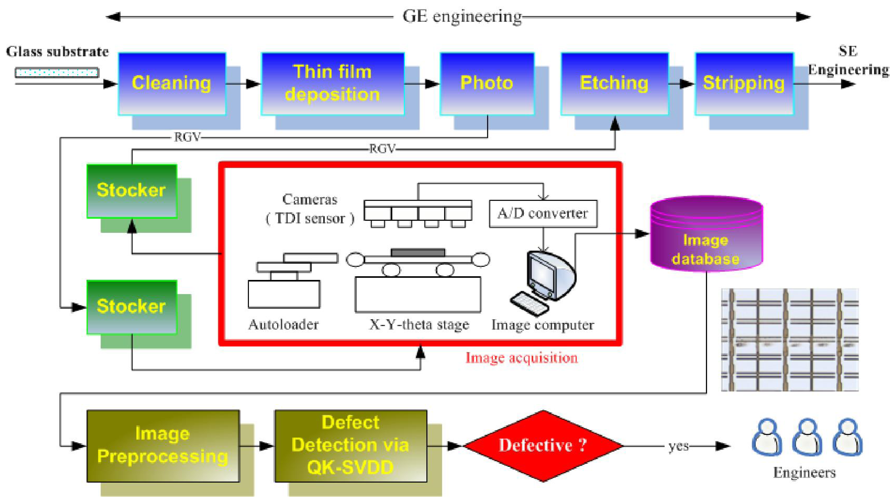
2.2. Overview of the Defect Detection Scheme
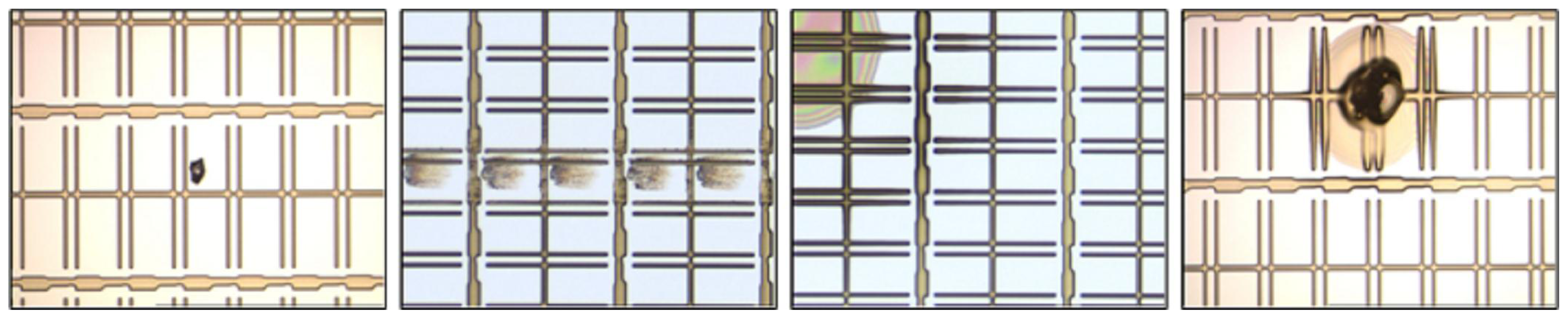
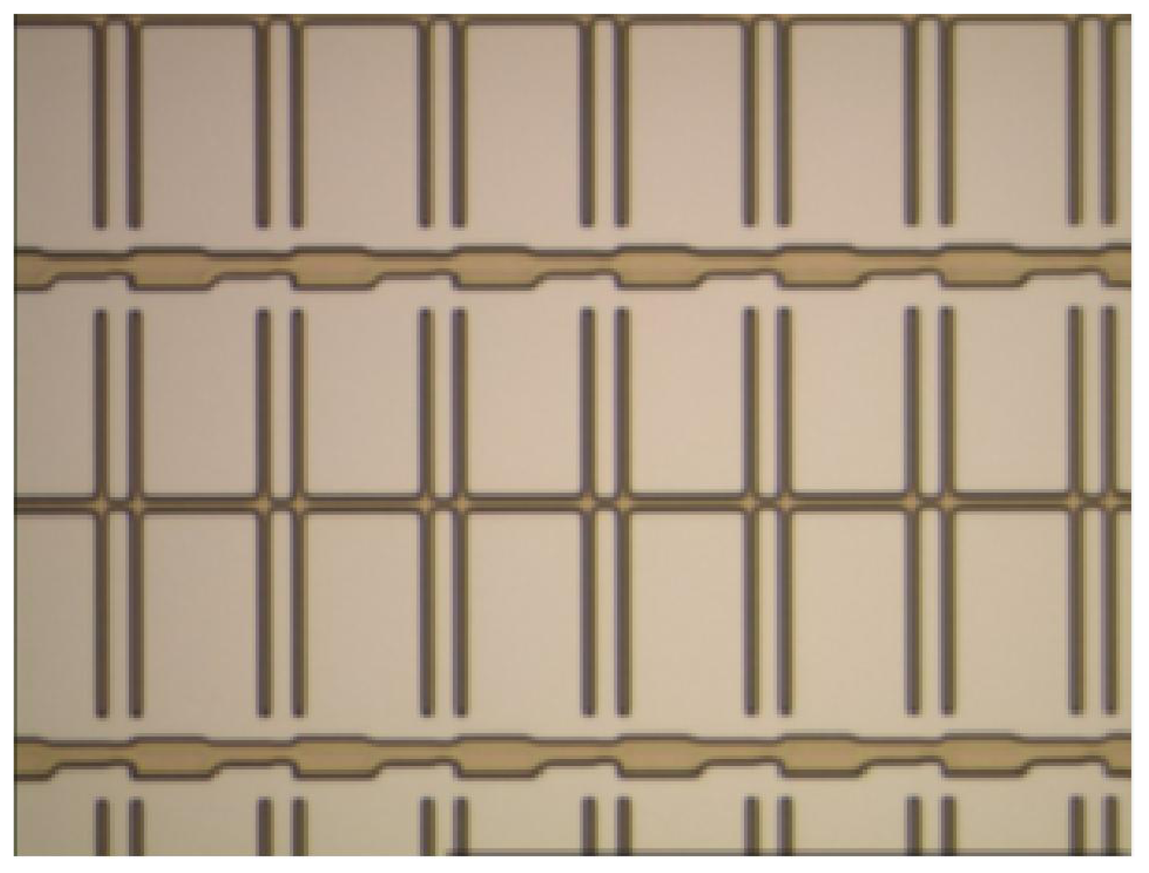
2.2.1. Image Acquisition
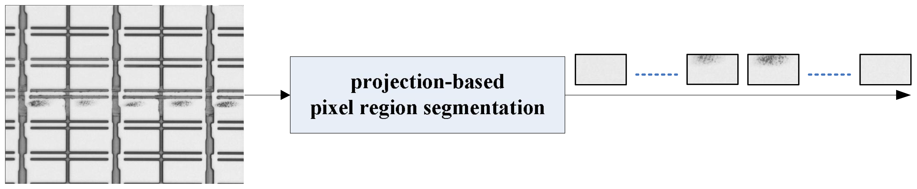
2.2.2. Image Preprocessing
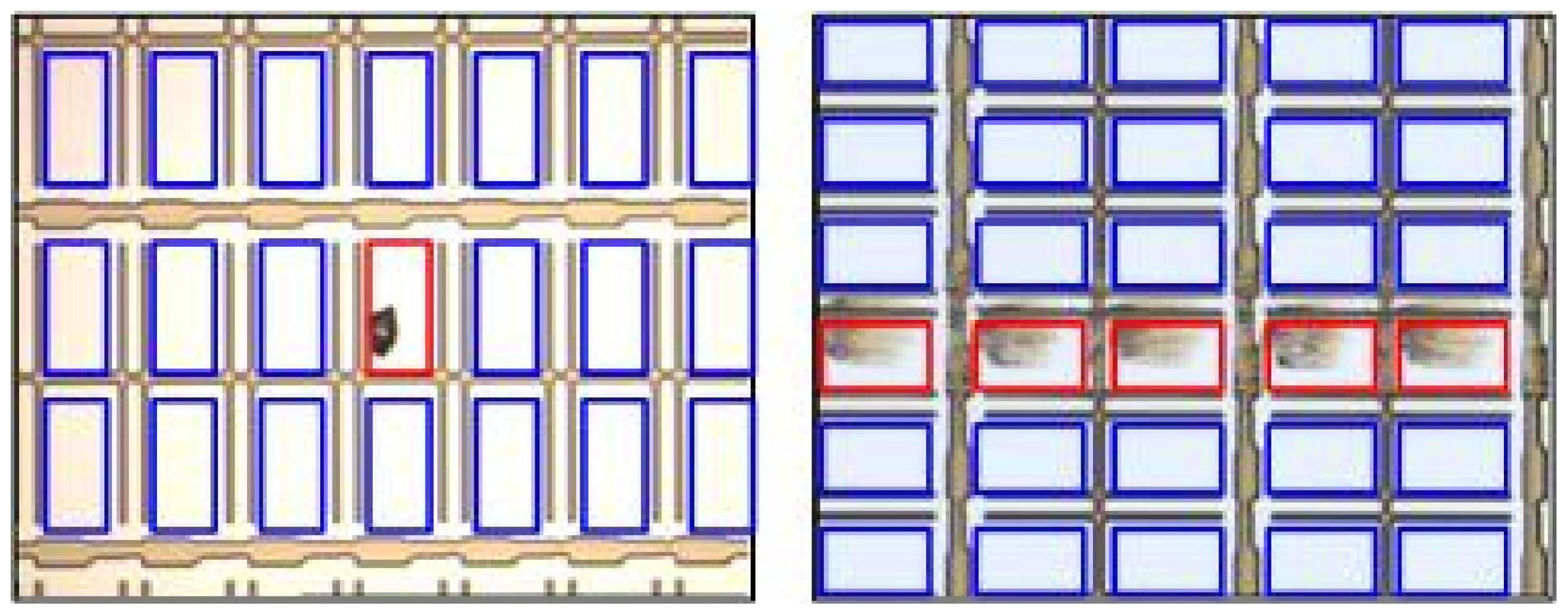
2.2.3. Defect Detection via QK-SVDD
2.3. SVDD
2.4. QK-SVDD
- First, an SVDD is initially trained on a target training set by a primary kernel, thereby producing a set of UBSVs and BSVs. The primary kernel is the Gaussian kernel.
- Second, the primary kernel is replaced by the quasiconformal kernel defined in equation (11).
- Then, retrain the SVDD with the quasiconformal kernel using the same target training set.
2.5. Comparison between Our Method and the Kernel Boundary Alignment (KBA) Algorithm
3. Experimental Section
Data
3.1. Comparison based on Balanced Test Sets
Training
Testing results
Speed
3.2. Comparison Based on Imbalanced Test Sets
4. Conclusions
References
- Song, YC; Choi, DH; Park, KH. Multiscale detection of defect in thin film transistor liquid crystal display panel. Jpn J Appl Phys 2004, 43, 5465–5468. [Google Scholar]
- Tsai, DM; Lin, PC; Lu, CJ. An independent component analysis-based filter design for defect detection in low-contrast surface images. Pattern Recognit 2006, 39, 1679–1694. [Google Scholar]
- Chen, LC; Kuo, CC. Automatic TFT-LCD mura defect inspection using discrete cosine transform-based background filtering and ‘just noticeable difference’ quantification strategies. Meas Sci Technol 2008, 19, 015507. [Google Scholar]
- Vapnik, VN. Statistical Learning Theory; Wiley-Interscience: Hoboken, NJ, USA, 1998. [Google Scholar]
- Markou, M; Singh, S. Novelty detection: A review, part I: Statistical approaches. Signal Process 2003, 83, 2481–2497. [Google Scholar]
- Markou, M; Singh, S. Novelty detection: A review, part II: Neural network based approaches. Signal Process 2003, 83, 2499–2521. [Google Scholar]
- Liu, YH; Huang, YK; Lee, MJ. Automatic inline-defect detection for a TFT-LCD array process using locally linear embedding and support vector data description. Meas Sci Technol 2008, 19, 095501. [Google Scholar]
- Roweis, ST; Saul, LK. Nonlinear dimensionality reduction by locally linear embedding. Science 2000, 290, 2323–2326. [Google Scholar]
- Tax, D; Duin, R. Support vector data description. Math Learn 2004, 54, 45–66. [Google Scholar]
- Liu, YH; Liu, YC; Chen, YZ. Fast support vector data descriptions for novelty detection. IEEE Trans Neural Netw 2010, 21, 1296–1313. [Google Scholar]
- Lee, K; Kim, DW; Lee, KH; Lee, D. Density-induced support vector data description. IEEE Trans Neural Netw 2007, 18, 284–289. [Google Scholar]
- Japkowicz, N (Ed.) AAAI Tech Report WS-00-05. Proceedings of the AAAI’2000 Workshop on Learning from Imbalanced Data Sets, Austin, TX, USA, 31 July 2000; AAAI: Menlo Park, CA, USA, 2000.
- Turney, P. Types of cost in inductive concept learning. Proceedings of the ICML’2000 Workshop on Cost-Sensitive Learning, Stanford, CA, USA, 29 June–2 July 2000.
- Japkowicz, N. Class imbalance: are we focusing on the right issue? Proceedings of the ICML’2003 Workshop on Learning from Imbalanced Data Sets, Washington, DC, USA, 21 August 2003.
- Chawla, NV; Japkowicz, N; Kolcz, A. Editorial: Special issue on learning from imbalanced data sets. ACM SIGKDD Explo Newsl 2004, 6, 1–6. [Google Scholar]
- Liu, XY; Wu, J; Zhou, ZH. Exploratory Under-Sampling for Class-Imbalance Learning. Proceedings of the 6th International Conference on Data Mining, Hong Kong, China, 18–22 December 2006; pp. 965–969.
- Jo, T; Japkowicz, N. Class imbalances versus small disjuncts. ACM SIGKDD Explor Newsl 2004, 6, 40–49. [Google Scholar]
- Chawla, NV; Bowyer, KW; Hall, LO; Kegelmeyer, WP. SMOTE: Synthetic minority over-sampling technique. J Artif Intell Res 2002, 16, 321–357. [Google Scholar]
- Chawla, NV; Lazarevic, A; Hall, LO; Bowyer, KW. SMOTE Boost: Improving Prediction of the Minority Class in Boosting. Proceedings of the Seventh European Conference on Principles and Practice of Knowledge Discovery in Databases, Cavtat-Dubrovnik, Croatia, 22–26 September 2003; pp. 107–119.
- Mease, D; Wyner, AJ; Buja, A. Boosted classification trees and class probability/quantile estimation. J Mach Learn Res 2007, 8, 409–439. [Google Scholar]
- Elkan, C. The Foundations of Cost-Sensitive Learning. Proceedings of the 17th International Joint Conference on Artificial Intelligence, Seattle, WA, USA, 4–10 August 2001; pp. 973–978.
- Ting, KM. An instance-weighting method to induce cost-sensitive trees. IEEE Trans Knowl Data Eng 2002, 14, 659–665. [Google Scholar]
- Sun, Y; Kamel, MS; Wong, AKC; Wang, Y. Cost-sensitive boosting for classification of imbalanced data. Pattern Recognit 2007, 40, 3358–3378. [Google Scholar]
- Veropoulos, K; Campbell, C; Cristianini, N. Controlling the Sensitivity of Support Vector Machines. Proceedings of the International Joint Conference on Artificial Intelligence, Stockholm, Sweden, July 31–August 6 1999; pp. 55–60.
- Kwok, JT. Moderating the outputs of support vector machine classifiers. IEEE Trans Neural Netw 1999, 10, 1018–1031. [Google Scholar]
- Liu, YH; Chen, YT. Face recognition using total margin-based adaptive fuzzy support vector machines. IEEE Trans Neural Netw 2007, 18, 178–192. [Google Scholar]
- Wang, BX; Japkowicz, N. Boosting Support Vector Machines for Imbalanced Data Sets. Proceedings of the 17th International Conference on Foundation of Intelligence System, Toronto, ON, Canada, 20–23 May 2008; 1994; pp. 38–47. [Google Scholar]
- Wu, G; Chang, EY. KBA: Kernel boundary alignment considering imbalanced data distribution. IEEE Trans Knowl Data Eng 2005, 17, 786–795. [Google Scholar]
- Japkowicz, N. Supervised versus unsupervised binary-learning by feedforward neural networks. Math Learn 2001, 42, 97–122. [Google Scholar]
- Manevitz, LM; Yousef, M. One-class SVMs for document classification. J Mach Learn Res 2001, 2, 139–154. [Google Scholar]
- Raskutti, B; Kowalczyk, A. Extreme re-balancing for SVMs: A case study. ACM SIGKDD Explor Newsl 2004, 6, 60–69. [Google Scholar]
- Lee, HJ; Cho, S. The novelty detection approach for difference degrees of class imbalance. Lect Note Comput Sci 2006, 4233, 21–30. [Google Scholar]
- Manevitz, L; Yousef, M. One-class document classification via neural networks. Neurocomputing 2007, 70, 1466–1481. [Google Scholar]
- He, H; Garcia, EA. Learning from imbalanced data. IEEE Trans Knowl Data Eng 2009, 21, 1263–1284. [Google Scholar]
- Hoffmann, H. Kernel PCA for novelty detection. Pattern Recognit 2007, 40, 863–874. [Google Scholar]
- Ryan, J; Lin, MJ; Miikkulainen, R. Jordan, MI, Kearns, MJ, Solla, SA, Eds.; Intrusion Detection with Neural Networks. In Advances in Neural Information Processing Systems; MIT Press: Cambridge, MA, USA, 1998; Volume 10, pp. 943–949. [Google Scholar]
- Campbell, C; Bennett, KP. A Linear Programming Approach to Novelty Detection. In Advances in Neural Information Processing Systems; MIT Press: Cambridge, MA, USA, 2001; Volume 13, pp. 395–401. [Google Scholar]
- Crammer, K; Chechik, G. A Needle in a Haystack: Local One-Class Optimization. Proceedings of the 21th International Conference on Machine Learning, Banff, Canada, 4–8 July 2004.
- Lanckriet, GRG; Ghaoui, LE; Jordan, MI. Robust Novelty Detection with Single-Class MPM. In Advances in Neural Information Processing Systems; MIT Press: Cambridge, MA, USA, 2003; Volume 15, pp. 929–936. [Google Scholar]
- Schölkopf, B; Platt, JC; Shawe-Taylor, J; Smola, AJ; Williamson, RC. Estimating the support of a high-dimensional distribution. Neural Comput 2001, 13, 1443–1471. [Google Scholar]
- Burges, CJC. Geometry and invariance in kernel based methods. In Advances in Kernel Methods—Support Vector Learning; Schölkopf, B, Burges, CJC, Smola, A, Eds.; MIT Press: Cambridge, MA, USA, 1999; pp. 89–116. [Google Scholar]
- Schölkopf, B; Smola, A. Learning with Kernels; MIT Press: Cambridge, MA, USA, 2002. [Google Scholar]
- Wu, S; Amari, S. Conformal transformation of kernel functions: A data-dependent way to improve support vector machine classifiers. Neural Process Lett 2002, 15, 59–67. [Google Scholar]
- Peng, J; Heisterkamp, DR; Dai, HK. Adaptive quasiconformal kernel nearest neighbor classification. IEEE Trans Pattern Anal Mach Intell 2004, 26, 656–661. [Google Scholar]
- Pan, JS; Li, JB; Lu, ZM. Adaptive quasiconformal kernel discriminant analysis. Neurocomputing 2008, 71, 2754–2870. [Google Scholar]
- Tsang, IW; Kwok, JT; Zurada, JM. Generalized core vector machines. IEEE Trans Neural Netw 2006, 17, 1126–1140. [Google Scholar]
- Weston, J; Schölkopf, B; Eskin, E; Leslie, C; Noble, S. Dealing with large diagonals in kernel matrices. Annals of the Institute of Statistical Mathematics 2003, 55, 391–408. [Google Scholar]
- Tsang, IW; Kwok, JT; Cheung, PM. Core vector machines: Fast SVM training on very large data sets. J Mach Learn Res 2005, 6, 363–392. [Google Scholar]
- Schölkopf, B; Smola, A; Müller, KR. Nonlinear component analysis as a kernel eigenvalue problem. Neural Comput 1998, 10, 1299–1319. [Google Scholar]


| Methods | Average TRR (in %) | Average OAR (in %) | Average ER (in %) |
|---|---|---|---|
| SVDD | 1.10 (±0.34) | 12.80 (±2.74) | 6.95 |
| QK-SVDD | 0.90 (±0.27) | 10.70 (±1.95) | 5.80 |
| Methods | Average TRR (in %) | Average OAR (in %) | Average ER (in %) |
|---|---|---|---|
| SVDD | 5.60 (±1.54) | 6.10 (±2.14) | 5.85 |
| QK-SVDD | 4.40 (±1.34) | 3.60 (±1.74) | 4.00 |
| Average Training Time (s) | Average Testing Time (ms/PR) | |
|---|---|---|
| SVDD | 0.623 | 2.16 |
| QK-SVDD | 1.468 | 2.38 |
| Methods | Average TRR (in %) | Average OAR (in %) | Average BL (in %) |
|---|---|---|---|
| SVDD | 0.92 (±0.44) | 11.60 (±2.71) | 6.26 |
| QK-SVDD | 0.89 (±0.41) | 10.10 (±1.69) | 5.45 |
| Methods | Average TRR (in %) | Average OAR (in %) | Average BL (in %) |
|---|---|---|---|
| SVDD | 5.23 (±1.23) | 5.58 (±1.87) | 5.41 |
| QK-SVDD | 4.21 (±1.08) | 3.70 (±1.77) | 3.96 |
| Methods | Average TRR (in %) | Average OAR (in %) | Average BL (in %) |
|---|---|---|---|
| SVDD | 9.81 (±1.95) | 2.20 (±1.01) | 6.01 |
| QK-SVDD | 7.54 (±1.31) | 0.80 (±0.43) | 4.17 |
© 2011 by the authors; licensee MDPI, Basel, Switzerland. This article is an open-access article distributed under the terms and conditions of the Creative Commons Attribution license (http://creativecommons.org/licenses/by/3.0/).
Share and Cite
Liu, Y.-H.; Chen, Y.-J. Automatic Defect Detection for TFT-LCD Array Process Using Quasiconformal Kernel Support Vector Data Description. Int. J. Mol. Sci. 2011, 12, 5762-5781. https://doi.org/10.3390/ijms12095762
Liu Y-H, Chen Y-J. Automatic Defect Detection for TFT-LCD Array Process Using Quasiconformal Kernel Support Vector Data Description. International Journal of Molecular Sciences. 2011; 12(9):5762-5781. https://doi.org/10.3390/ijms12095762
Chicago/Turabian StyleLiu, Yi-Hung, and Yan-Jen Chen. 2011. "Automatic Defect Detection for TFT-LCD Array Process Using Quasiconformal Kernel Support Vector Data Description" International Journal of Molecular Sciences 12, no. 9: 5762-5781. https://doi.org/10.3390/ijms12095762
APA StyleLiu, Y.-H., & Chen, Y.-J. (2011). Automatic Defect Detection for TFT-LCD Array Process Using Quasiconformal Kernel Support Vector Data Description. International Journal of Molecular Sciences, 12(9), 5762-5781. https://doi.org/10.3390/ijms12095762