Article

Beef Traceability Between China and Argentina Based on Various Machine Learning Models

1
Research Institute for Doping Control, Shanghai University of Sport, Shanghai 200438, China
2
Technical Center for Animal, Plant and Food Inspection and Quarantine, Shanghai Customs, Shanghai 201210, China
3
Shanghai Entry and Exit Food and Feed Safety Professional Service Platform, Shanghai 201210, China
4
Food Technology Institute-Agroindustry Research Center, Hurlingham 1686, Buenos Aires, Argentina
5
Institute of Science and Technology of Sustainable Food Systems, Hurlingham 1686, Buenos Aires, Argentina
*
Authors to whom correspondence should be addressed.
Molecules 2025, 30(4), 880; https://doi.org/10.3390/molecules30040880
Submission received: 17 January 2025 / Revised: 3 February 2025 / Accepted: 6 February 2025 / Published: 14 February 2025
(This article belongs to the Special Issue Applications of Spectroscopic Techniques in Food Sample Analysis)

Abstract

:
Beef, as a nutrient-rich food, is widely favored by consumers. The production region significantly influences the nutritional value and quality of beef. However, current methods for tracing the origin of beef are still under development, necessitating effective approaches to ensure food safety and meet consumer demand for high-quality beef. This study aims to establish a classification model for beef origin prediction by analyzing elemental content and stable isotopes in beef samples from two countries. The concentrations of elements in beef were analyzed using ICP-MS and ICP-OES, while the stable carbon isotope ratio was determined using EA-IRMS. Machine learning algorithms were employed to construct classification prediction models. A total of 83 beef samples were analyzed for the concentrations of 52 elements and the stable carbon isotope ratio. The classification accuracy of the PLS-DA model built on these results was 98.8%, while the prediction accuracy was 94.12% for the convolutional neural network (CNN) and 82.35% for the Random Forest algorithm. The PLS-DA model demonstrated higher classification accuracy compared to CNN and Random Forest, with an explanatory power (R2) of 0.924 and predictive ability (Q2) of 0.787. Combining the analysis of 52 elements and the stable carbon isotope ratio with machine learning algorithms enables effective tracing and origin prediction of beef from different regions. Key factors influencing beef origin were identified as Fe, Cs, As, δ13C, Co, V, Sc, Rb, and Ru.

Graphical Abstract

1. Introduction

Beef, as a common type of meat, is widely favored for its unique flavor and rich nutritional value. With increasing economic development, the demand for beef has surged, accompanied by higher consumer expectations for its safety and quality [1]. Argentina is one of the world’s leading beef exporters, predominantly raising Angus cattle through grass-fed practices—both essential attributes of premium-quality beef [2]. In 2023, Argentina exported 683,000 tons of beef globally, with China importing 527,000 tons, accounting for 79% of Argentina’s beef exports, making China its largest beef importer. Due to the high economic value of beef, cases of beef origin fraud are prevalent, causing financial losses and health risks to consumers. For example, some unscrupulous vendors sell beef from low-cost origins as high-priced origin products or adulterate beef with chicken, duck, or pork to increase profit margins [3,4]. Additionally, the illegal use of steroid hormones like trenbolone and clenbuterol during cattle farming to boost yield poses health risks to consumers. For professional athletes, consuming such beef could lead to a positive doping test, potentially jeopardizing their careers [4,5].
Traditional methods for tracing beef origin suffer from low accuracy and limited capability to identify actual production regions, leaving loopholes in food safety [6]. As the beef market continues to expand, it is increasingly crucial to develop efficient origin-tracing methods to ensure the safety of beef production and consumption. Meat traceability primarily relies on isotope and elemental analysis techniques. Environmental factors such as soil, water, and climate leave unique elemental and isotopic “fingerprints” in the muscle tissue of cattle. By analyzing these characteristics, the geographical origin of beef can be inferred. Stable isotope and elemental analyses are commonly used, with EA-IRMS (Elemental Analysis–Isotope Ratio Mass Spectrometry) and ICP-MS/OES (Inductively Coupled Plasma Mass Spectrometry/Optical Emission Spectrometry) being the most prevalent tools [7]. EA-IRMS measures isotope ratios of elements like carbon, nitrogen, hydrogen, and oxygen by combusting samples into their elemental components [8]. The carbon isotope ratio (δ13C) reflects the photosynthetic pathways of plants consumed by the cattle, providing insights into their feed sources [9]. Carbon isotopic characteristics of beef can distinguish between grass-fed and grain-fed beef and identify the cattle’s rearing environment. Argentina’s cattle are predominantly grass-fed, relying on pastures (C3 plants), which use the Calvin cycle for photosynthesis [10]. The carbon isotope ratio of C3 plants typically ranges from −22‰ to −30‰, reflecting a preference for the lighter carbon isotope (12C) over the heavier isotope (13C). In contrast, Chinese cattle are mainly grain-fed, with feed derived from corn, sorghum, and other C4 plants that employ the Hatch–Slack pathway for photosynthesis. C4 plants exhibit δ13C values of −10‰ to −14‰, and these differences in feed ultimately result in distinct isotopic fingerprints in the beef, providing a natural traceability tool [11,12,13].
In recent years, machine learning, a cornerstone of artificial intelligence, has emerged as a powerful tool for data processing, analysis, and prediction in food science [14,15]. PLS-DA (Partial Least Squares–Discriminant Analysis) is a multivariate statistical method widely applied in food traceability for its ability to extract relevant features from high-dimensional data and classify the origin and variety of food accurately [16]. It is particularly suitable for handling complex chemical data, such as spectral analysis and isotope ratios, and has been extensively used in the traceability of wine, tea, and olive oil [17]. For instance, in 2021, Xu et al. analyzed the carbon, nitrogen, and oxygen isotope ratios, 51 elements, and 35 fatty acids in milk powder samples from three regions, constructing a stable multivariate model (R2X = 0.693, Q2 = 0.854) for origin identification [18]. In 2022, Dehelean et al. measured the carbon, hydrogen, and oxygen isotope ratios and 28 elements in Romanian pork and chicken samples, using PLS-DA to establish traceability models with accuracies of 71.8% and 93.8%, respectively, and feeding style identification models with accuracies of 100% and 98% [19]. Convolutional neural networks (CNNs), a deep learning model, are increasingly used in food traceability due to their ability to efficiently extract local and global features through convolution and pooling operations [20]. In one study, Weng et al. utilized CNNs alongside support vector machines, Random Forests, and K-nearest neighbors (KNN) to analyze hyperspectral imaging data of lamb, successfully constructing geographical origin and breed identification models [21]. Random Forests, a decision tree-based ensemble learning method, are another popular machine learning approach in food science [22]. For example, Elisabete A. et al. analyzed elemental data from beef samples from five Brazilian regions, using Random Forests, multilayer perceptrons, and regression trees to classify beef origins, confirming significant regional differences in Brazilian beef [23].
This study addresses the critical need for robust food traceability systems by developing an innovative origin verification approach for beef products. Integrating multi-regional sampling from China and Argentina with advanced analytical techniques (ICP-MS, ICP-OES for 52 elemental profiles, and EA-IRMS for carbon stable isotope ratios), we established a comprehensive analytical framework that significantly enhances geographical discrimination accuracy. The creation of a machine learning-powered classification model not only demonstrates high-precision origin identification between these major beef-producing nations but also establishes a suitable methodology combining multi-elemental fingerprinting with stable isotope analysis. This breakthrough provides both technical support for combating food fraud and a scientific foundation for global meat traceability protocols while advancing the application of chemometric approaches in food authentication. Subsequent research will focus on model optimization for wider geographical coverage and the integration of complementary biomarkers to strengthen verification reliability.

2. Results

2.1. Analysis of Elemental Data

Using ICP-MS and ICP-OES, we determined the concentrations of 52 elements in 83 beef samples. The results are summarized in Table 1.
Among the 52 elements, 23 elements showed significant differences (p < 0.005), including Mg, P, Sc, K, V, Fe, Co, As, Rb, Ru, Rh, Cs, La, Ce, Nd, Sm, Eu, Gd, Tb, Dy, Yb, Tl, and Pb. The p-values for K, Fe, Rb, and Cs were less than 0.0001.
The observed differences in magnesium (Mg) content may be attributed to the prevalence of hypomagnesemia in cattle from central Argentina, which results in lower magnesium levels in Argentine beef compared to Chinese beef [24]. Significant differences in elements such as Fe, Cs, and Co have also been confirmed through molecular activation analysis and machine learning [25]. Additionally, previous studies have indicated that elements such as Dy, Fe, Rb, Tl, V, and 14 other elements are important factors for identifying the geographical origin of beef in traceability studies across different countries [26]. Combining findings from other studies with our experimental results, it can be concluded that there are significant differences in the elemental composition of beef from China and Argentina.

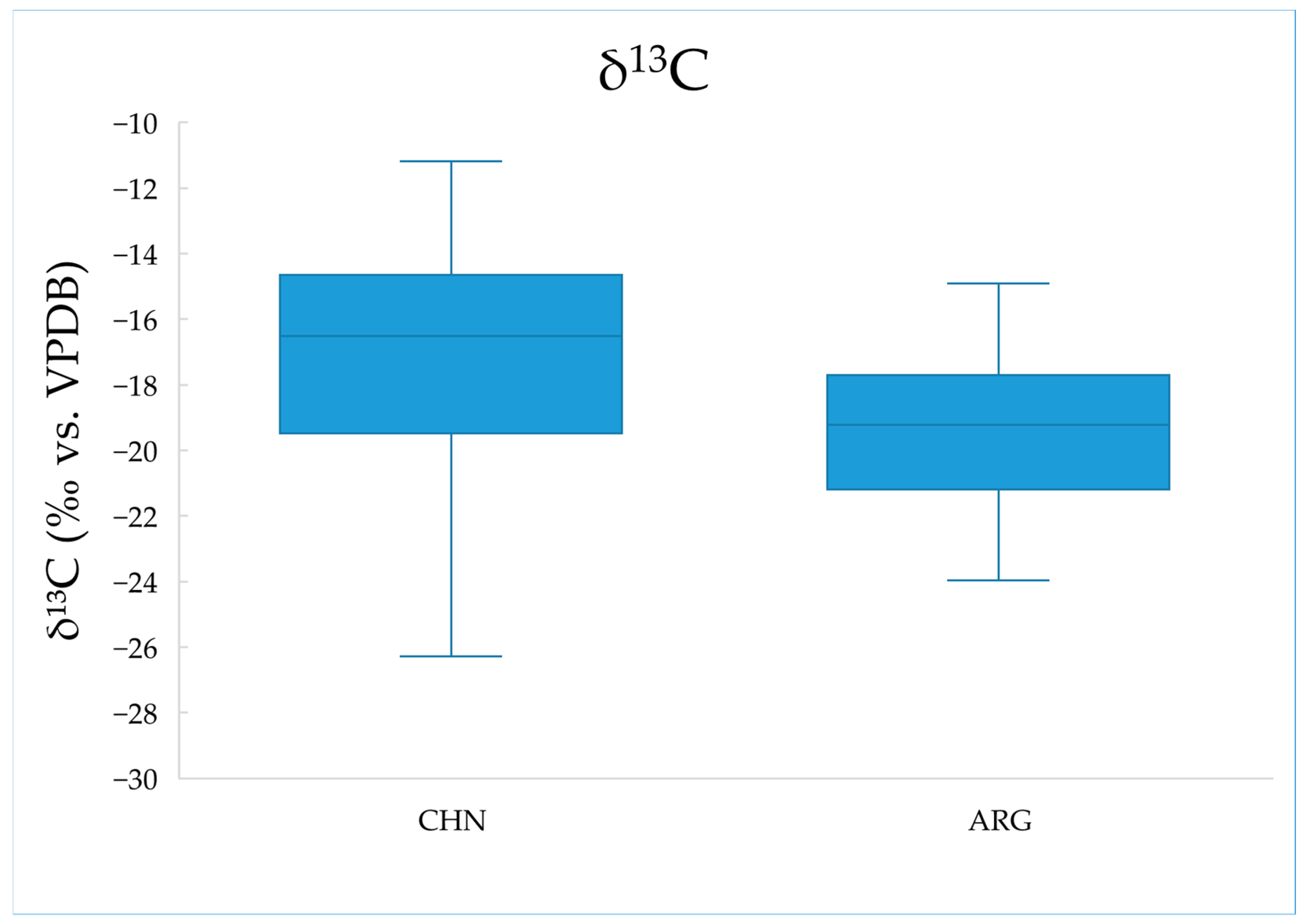
2.2. Analysis of Carbon Stable Isotope Ratios

We measured the carbon stable isotope ratios of 83 samples. The mean δ13C values and standard deviations of samples from China and Argentina are summarized in Table 2. A boxplot illustrating the δ13C distribution is shown in Figure 1.
Through the measurement of samples, we found that the δ13C values of beef samples from China range from −27.23‰ to −11.18‰, while those from Argentina range from −23.97‰ to −14.91‰, with average values of −17.52‰ and −19.58‰, respectively. The standard deviation of the carbon stable isotope ratio in Argentine beef samples was 2.42, whereas the standard deviation of Chinese beef samples was larger, at 3.81. The boxplot (Figure 2) shows that the δ13C values of Argentine beef are lower and more concentrated, while those of Chinese beef are higher and more dispersed. The standard deviation of Chinese beef is larger compared to Argentine beef, and the range between the maximum and minimum values is also greater, confirming the more uniform farming practices of Argentine cattle compared to China. In Argentina, most cattle are fed with C3 plants during the rearing process, resulting in a lower average δ13C value in Argentine beef compared to Chinese beef. In contrast, cattle farming methods in China are more diverse in terms of geography and feeding practices. China has both grass-fed cattle primarily fed on C3 plants and grain-fed cattle that are often provided with C4 plants as feed. As a result, the average δ13C value of Chinese beef is higher than that of Argentine beef [27,28,29]. There is a significant difference in δ13C values between Chinese and Argentine beef, suggesting that δ13C could serve as a potential indicator for distinguishing beef origins among the existing analysis variables.

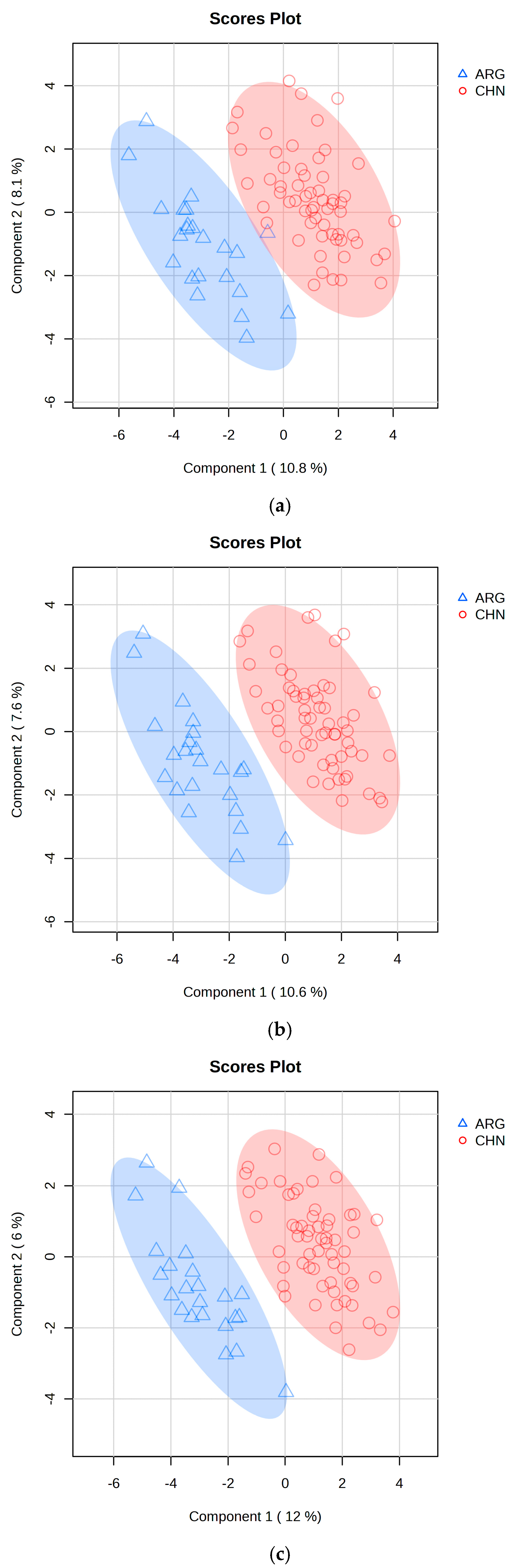
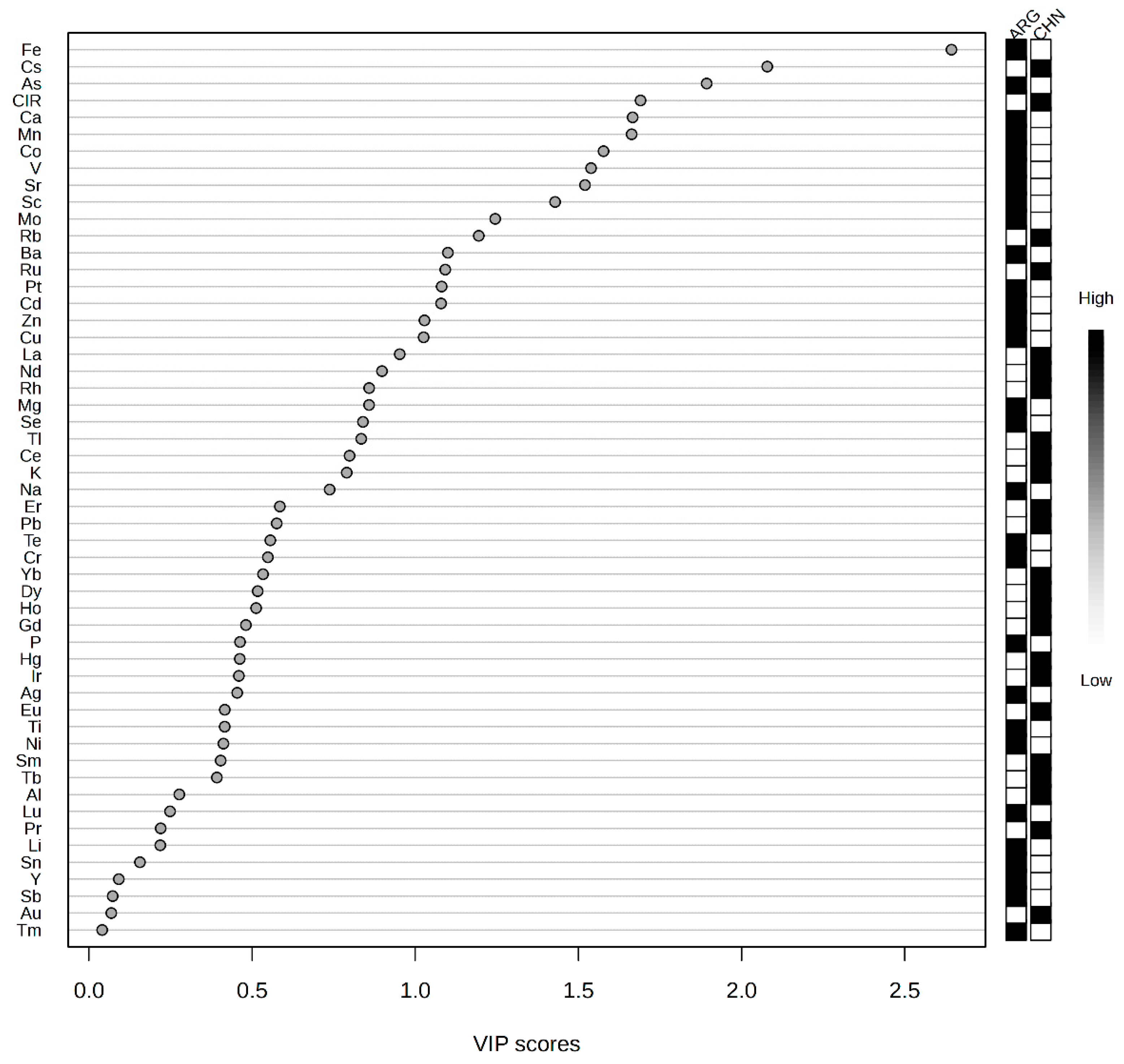
2.3. PLS-DA Classification Model

The classification model is shown in Figure 2a. We constructed the PLS-DA classification model using the elemental content data of beef samples. In the model, the samples are clearly divided into two clusters, with a 95% confidence interval serving as the threshold to differentiate the beef samples from the two regions. K-fold cross-validation is an effective method for evaluating PLS-DA models. In k-fold cross-validation, the original dataset or training dataset is divided into k folds (subsets), and the model is trained k times (iterations), resulting in k performance estimates. In each iteration, one fold (validation set) is used to evaluate the model, and the remaining k-1 folds are used for training. In this study, due to the sample size being less than 100, 10-fold cross-validation was chosen to obtain the best cross-validation results [30,31]. Performance evaluation depends on the accuracy, R2 (coefficient of determination), and Q2 (predictive R2) obtained from the 10 validation iterations. These represent the proportion of correctly classified samples out of the total number of samples, the degree of fit between the model and the training data, and the model’s ability to predict unseen data. Among these, Q2 reflects the model’s predictive performance in cross-validation. A high Q2 value indicates that the model not only fits well on the training set but also has good predictive capability on new data [32]. When using the 52 elemental content features as variables, the classification accuracy for the beef from the two regions was 97.8%, with an R2 of 0.915 and a Q2 of 0.706.
The PLS-DA model can also optimize classification results by removing redundant variables. The classification ability of the PLS-DA model depends on the correlation between the variables and the class labels. If there are many irrelevant or redundant variables, they may be treated as noise and introduced into the model, which could interfere with the model, reducing its performance and robustness [33,34,35]. VIP (Variable Importance in Projection) is an indicator used to assess the importance of each variable (feature) to the model. It helps identify which variables contribute most to the model’s predictive ability, allowing the selection of variables that have the most impact on classification or regression results. Variables with low VIP values are less important to the model and can be discarded to improve classification accuracy [36,37]. By evaluating the VIP values of the model and re-modeling, redundant variables such as Tm, Au, Pr, Sb, Y, Tb, Eu, and Sm, which contribute less to the model, were removed. The classification model results after this adjustment are shown in Figure 2c. From the results, it can be seen that the samples within the same region are now more tightly clustered, the 95% confidence interval has narrowed, and the differentiation between regions is more prominent. The 10-fold cross-validation results are shown in Table 2, where the classification accuracy for beef from the two regions is 98.8%, with an R2 of 0.925 and a Q2 of 0.787. Compared to the model trained with single-variable data, R2 and Q2 have improved by 1.05% and 11.47%, respectively. This demonstrates that removing redundant variables significantly enhances the model’s predictive capability.
In addition, in the PLS-DA model, variables with higher VIP values contribute more to the model. Therefore, VIP values can serve as an important criterion for selecting key influencing factors of beef origin [38,39]. Figure 3 shows the ranking of VIP scores in this PLS-DA model. In this study, variables with VIP scores greater than 1.0, such as Fe, Cs, As, δ13C, Ca, Mn, Co, V, Sr, Sc, Mo, Rb, Ba, Ru, Pt, Cd, Zn, and Cu, significantly contribute to the model. These variables can be considered key influencing factors for beef origin. Among them, Fe is the most distinct variable. Fe, Cs, As, Co, V, Sc, Rb, and Ru are also the elements with the largest differences in the element data t-test results (p > 0.05). However, not every element with a large t-test result is a key influencing factor. This is because VIP values take into account not only the significance of variables but also their explanatory power within the model. If a variable contributes little to the overall variation in the model, and factors such as small sample size or data imbalance cause certain variables to appear significant in t-tests but not adequately represent their importance in multivariate model analysis, even if they are significant in individual t-tests, their VIP values might still be low. For instance, Rh is one such example. δ13C ranks fourth in the VIP value list, indicating that carbon stable isotope ratios are a significant contributor to this classification model and are a crucial factor in distinguishing beef from different regions.

2.4. CNN Classification Model

The convolutional neural network (CNN) classification model was constructed using the TensorFlow library with Python 3.12.6, with the sample data randomly split into training and test sets in an 80:20 ratio. CNNs achieve efficient feature learning and classification prediction by extracting local features from the input data and progressively abstracting them through multiple layers. The basic structure of the model consists of the input layer, convolutional layers, pooling layers, fully connected layers, activation functions, and the output layer. The input layer receives the raw data, the convolutional layers use filters (kernels) to extract local features, the pooling layers reduce the dimensionality of the feature maps, the fully connected layers map the extracted features to classification results, the ReLU activation function introduces non-linearity, and the output layer produces the classification probability or class labels based on the specific task. Based on the dataset characteristics, two convolutional layers were used to extract features, two pooling layers were employed to reduce dimensions, two Dropout layers were added to prevent overfitting, and two fully connected layers were utilized to complete the classification prediction. Finally, the Softmax activation function was applied to convert the output into a probability distribution over the classes, thus completing the CNN classification model [40,41,42].
The results of the classification model trained on the training set are visualized in Figure 4. As can be seen, after feature extraction, the dataset shows a clear trend of classification. While the CNN model’s predictive ability cannot be fully visualized in a 3D plot, PCA can still be used to preliminarily assess the CNN’s ability to extract features. The prediction results for the test set are shown in Table 3. It is evident that the CNN performs excellently in classifying the test samples. Out of 17 samples, only 1 was classified incorrectly, yielding an overall accuracy of 94.12%. Moreover, the confidence for most correctly predicted samples was over 90%.

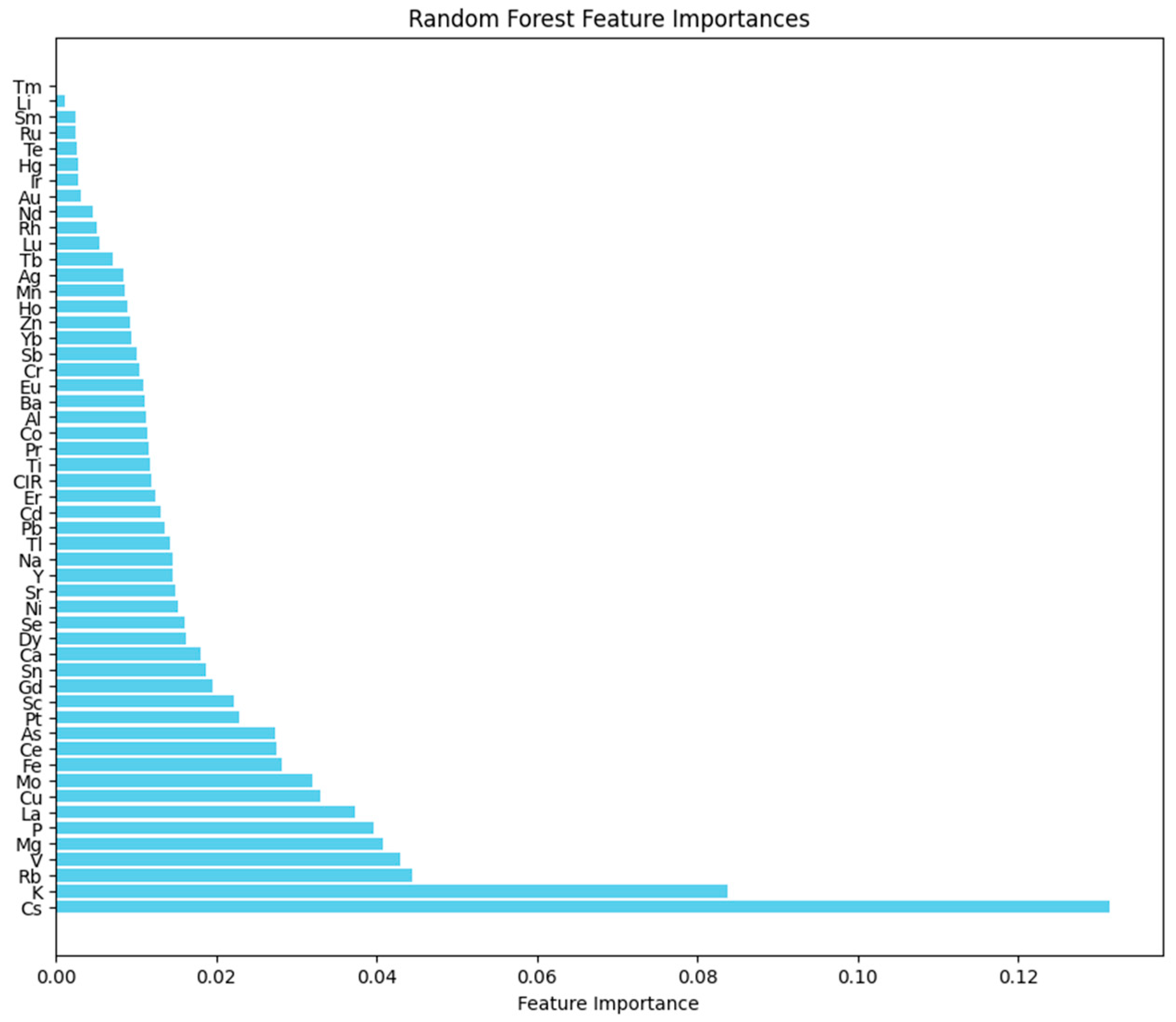
2.5. Random Forest Classification Model

The classification prediction results for the test set are shown in Table 4. In this study, 100 decision trees were used to construct the Random Forest classification model. Typically, the more trees in the model, the more stable its performance, though the computational time also increases. The training classification accuracy of this model was 100%, and the validation set accuracy was 78.57%. The model’s classification prediction ability is weaker than that of the CNN model. For Argentine beef classification, the accuracy was 100%, while for Chinese beef samples, the accuracy was 40%, resulting in an overall prediction accuracy of 82.35%.
In the Random Forest algorithm, feature importance is used to assess the contribution of each sample attribute to the classification model (Figure 5) [43,44]. The top ten ranked variables in terms of importance are Cs, K, Rb, V, Mg, P, La, Cu, Mo, and Fe. Among these, K, Cs, Rb, V, Mg, P, La, and Fe overlap with the VIP values from the PLS-DA model and the elements with the most significant differences in the elemental data. Therefore, these eight variables are key factors that differentiate beef origin. The Random Forest Feature Importances are shown in Figure 5, where the contribution of sample attributes to the model is ranked from smallest to largest. The top ten variables in terms of importance are Cs, K, Rb, V, Mg, P, La, Cu, Mo, and Fe. The classification prediction results for the test set are presented in Table 5, with an overall prediction accuracy of 82.35%.
Overall, significant differences exist between Chinese and Argentine beef in terms of elemental content and carbon isotope levels, and these differences can be utilized to construct classification models through machine learning, enabling accurate beef classification. Among all the models used in this study, the PLS-DA model constructed using MetaboAnalyst achieved the highest classification accuracy (97.5%), followed by the CNN model (94.12%) and the Random Forest model (82.35%). By selecting variables with VIP values greater than 1 from the PLS-DA model, as well as variables with significant differences in elemental and carbon stable isotope analysis results (p < 0.05), a Venn diagram was constructed. The results are shown in Figure 6. This method identified nine key variables: Fe, Cs, As, δ13C, Co, V, Sc, Rb, and Ru. These variables show significant differences between the beef samples from the two regions and contribute significantly to the origin traceability model. Therefore, these nine variables can be regarded as key influencing factors for beef origin traceability.

3. Material and Methods

3.1. Materials and Reagents

HPLC-grade methanol was purchased from TEDIA (Fairfield, OH, USA). Chloroform (analytical grade) was obtained from Sinopharm Chemical Reagent Co., Ltd. (Beijing, China). IAEA-600 caffeine (δ13C = −27.771‰) was supplied by the International Atomic Energy Agency (Vienna, Austria). Standard solutions of Ir, Pt, Au, Ag, V, Co, Te, Rb, Ru, Cs, and As (1000 µg/mL) and four internal standards (Ge, Rh, In, and Bi) were purchased from o2si (South Carolina, NC, USA). Standard solutions for other elements (1000 µg/mL) and nitric acid were procured from the National Nonferrous Metals and Electronic Materials Analysis and Testing Center (Beijing, China).

3.2. Methods

3.2.1. Sample Collection

Beef samples were collected from local markets in various regions of Argentina and provinces of China. A total of 83 beef samples were collected, including 60 samples from different provinces in China (Heilongjiang, Jilin, Xinjiang, Gansu, Inner Mongolia, Henan, Yunnan, Ningxia, Qinghai, Jiangsu, Sichuan, and Shandong) and 23 samples from different provinces in Argentina (Buenos Aires, Santa Fe, La Pampa, and Entre Ríos). After the sample collection, they were stored in a −20 °C freezer, and the subsequent analysis was completed within 30 days.

3.2.2. Preparation for Elemental Determination

To determine the elemental content of beef samples, appropriate preprocessing was conducted to meet ICP-MS/OES requirements. Using microwave digestion, 1.0 g of each beef sample (accurate to 0.001 g) was weighed and treated according to the national standard GB 5009.268-2016 [45]. Five milliliters of nitric acid were added to the weighed samples, followed by sealing and vortexing for 30 s. The samples were then placed in a preheated microwave digestion system. The digestion program was set as follows: initial temperature of 120 °C held for 5 min, increased to 150 °C for 10 min, and then raised to 190 °C for 20 min. After digestion, the mixture was cooled to room temperature, filtered using a funnel to remove solid residues, and diluted to 50 mL with deionized water for analysis.

3.2.3. Preparation for Carbon Stable Isotope Ratio Determination

Since isotope fractionation occurs during fat synthesis, and fat content varies across beef samples, defatting was necessary to eliminate the influence of fat on carbon isotope ratio determination. For this, 300 g of beef sample was minced, and 15.0 g of each sample was evenly spread in a petri dish. The samples were freeze-dried at −45 °C using a benchtop freeze-dryer and then ground into powder. Following the rapid sample preparation method for beef isotope determination by Zhao et al. [46], 5 mL of a chloroform–methanol solution (2:1, v:v) was added to the powdered sample in a centrifuge tube. The mixture was vortexed for 10 min (2500 rpm) and centrifuged at 4 °C using an Eppendorf 5810R centrifuge. The fat-containing supernatant was discarded, and the solid residue was collected. This defatting process was repeated twice. Finally, the samples were dried overnight in an oven at 50 °C. Using a microanalytical balance (XPE26C, Mettler Toledo, Switzerland), 80–130 µg of defatted, dried sample powder was weighed into tin capsules (Sn, 8 mm × 5 mm, Thermo Fisher, Waltham, MA, USA), sealed, and formed into a ball for carbon isotope ratio determination. Each sample was measured six times, and the mean value was used for accurate δ13C determination.

3.2.4. Elemental Measurements by ICP-OES and ICP-MS

The elemental content of beef samples was measured using an Agilent 5100 ICP-OES (Agilent Technologies, Santa Clara, CA, USA) for Na, K, Mn, P, Zn, Ca, Fe, and Mg, while 44 other elements were analyzed using an Agilent 7900 ICP-MS (Agilent Technologies, USA). Each sample was analyzed in duplicate for all element measurements.
Parameters for ICP-OES included the following: replicate time of 3, pump speed of 12 rpm, uptake delay of 15 s, reading time of 3 s, RF power of 1.2 kW, stabilization time of 10 s, and observation modes (radial and axial simultaneous view). The plasma gas flow rate was set to 12.0 L/min, the nebulizer gas flow rate to 0.70 L/min, the auxiliary gas flow rate to 1.00 L/min, and the additional air flow rate to 0.00 L/min. The detection range was 0.01–0.7 mg/100 g and 0.03–3 mg/100 g.
Parameters for ICP-MS included the following: peak hopping scan mode, 3 points per peak, reading time of 3 s, sample depth of 10 mm, spray chamber temperature of 2 °C, sample uptake speed of 0.5 r/s, carrier gas and hydrogen gas flow rates of 0.82 mL/min and 4 mL/min, dilution plasma flow rate of 0.3 L/min, and RF power of 1600 W. The detection and calibration ranges were 0.03 µg/kg to 0.5 mg/kg and 0.1 µg/kg to 2 mg/kg, respectively.

3.2.5. δ13C Measurements by EA-IRMS

Carbon stable isotope ratios (δ13C) of beef samples were measured using EA-IRMS (Delta V Advantage, Thermo Scientific, Waltham, MA, USA), with each sample analyzed six times. The obtained δ13C values were normalized to the international standard Vienna Pee Dee Belemnite (V-PDB) using laboratory working standards calibrated against V-PDB. Parameters for the elemental analyzer were as follows: oxidation furnace temperature of 980 °C, column temperature of 50 °C, helium carrier gas flow rate of 100 mL/min, oxygen flow rate of 175 mL/min, helium purge gas flow rate of 180 mL/min, and oxygen injection time of 4 s. IRMS conditions included the following: electron ionization mode (EI), ion source voltage of 3.07 kV, vacuum of 1.6 × 10⁻⁶ mbar, and gas pressures of 4 bar (helium, oxygen, carbon dioxide) and 8 bar (air). The δ13C values were expressed in per mil (‰) as follows: δ = [(Rsample − Rstandard)/Rstandard] × 1000, where R represents the 13C/12C ratio of the sample or standard. To ensure accuracy and stability, IAEA-600 (caffeine, δ13C = −27.771‰) was used to calibrate the instrument. The average deviation between measured and standard values was less than 0.3‰, and the standard deviation of parallel measurements was below 0.3‰.

3.2.6. Statistical Analysis

The data were statistically analyzed using Microsoft Excel, with the t-test performed using Welch’s t-test, and the two-tailed p-value was calculated. PLS-DA combines the advantages of Principal Component Analysis (PCA) and Partial Least Squares (PLS) regression and is a supervised learning method for handling multivariate data. It is suitable for classification tasks when there are significant correlations and collinearity between samples. We constructed the PLS-DA classification model using MetaboAnalyst 6.0. In the initial data preprocessing, we used log transformation and mean centering to normalize the raw data, making it easier for further analysis. The convolutional neural network (CNN) classification model was constructed using Python 3.12.6 and TensorFlow library, with the sample data randomly split into training and test sets in an 80:20 ratio. CNN achieves efficient feature learning and classification prediction by extracting local features from the input data and progressively abstracting them through multiple layers. The basic structure of the model consists of the input layer, convolutional layers, pooling layers, fully connected layers, activation functions, and the output layer. The input layer receives the raw data, the convolutional layers use filters (kernels) to extract local features, the pooling layers reduce the dimensionality of the feature maps, the fully connected layers map the extracted features to classification results, the ReLU activation function introduces non-linearity, and the output layer produces the classification probability or class labels based on the specific task. Based on the dataset characteristics, two convolutional layers were used to extract features, two pooling layers were employed to reduce dimensions, two Dropout layers were added to prevent overfitting, and two fully connected layers were utilized to complete the classification prediction. Finally, the Softmax activation function was applied to convert the output into a probability distribution over the classes, thus completing the CNN classification model. The Random Forest classification model was constructed using Python 3.12.6 and the Scikit-learn library, with the sample data randomly split into training and external test sets in an 80:20 ratio. Random Forest is based on the decision tree concept, where multiple decision trees are built, and their outputs are integrated to perform classification or regression analysis. The core idea is to combine several weak classifiers (decision trees) into a strong classifier, which improves the model’s accuracy and robustness.

4. Conclusions

This study evaluated the elemental and carbon stable isotope characteristics of 83 beef samples (60 from different regions in China and 23 from Argentina). Based on multi-element and stable isotope ratios, three classification prediction models—PLS-DA, convolutional neural network (CNN), and Random Forest—were established. The results showed that these three models were effective in distinguishing the origin of beef from China and Argentina. Among them, the PLS-DA model achieved the highest classification accuracy of 97.5%, with an R2 of 0.924 and a Q2 of 0.743, indicating strong model performance. The model analysis identified nine key influencing factors—Fe, Cs, As, δ13C, Co, V, Sc, Rb, and Ru—that had the greatest impact on beef origin traceability, providing valuable data support for further research on beef product traceability.

Author Contributions

Conceptualization, X.X., C.Z., D.C., B.L., and S.X.; Data curation, X.X.; Formal analysis, X.X. and S.X.; Funding acquisition, C.Z., D.C., and B.L.; Investigation, X.X.; Methodology, C.Z.; Project administration, B.L.; Resources, C.Z., D.C., B.L., and X.Y.; Software, S.X.; Supervision, B.L.; Visualization, X.X., B.L., and S.X.; Writing—original draft, X.X.; Writing—review and editing, C.Z., R.Z., J.Z., L.W., S.Z., D.C., B.L., and X.Y. All authors have read and agreed to the published version of the manuscript.

Funding

This research was funded by the National Key Research and Development Program of China (No. 2023YFE0106900) and the Collaborative Innovation Capacity Construction Project, Shanghai University of Sport (2023).

Institutional Review Board Statement

Not applicable.

Informed Consent Statement

Not applicable.

Data Availability Statement

Data will be made available on request.

Acknowledgments

The authors wish to thank anonymous reviewers for their constructive commentson the presentation of this article.

Conflicts of Interest

The authors declare that they have no known competing financial interests.

References

  1. Greenwood, P.L. Review: An overview of beef production from pasture and feedlot globally, as demand for beef and the need for sustainable practices increase. Animal 2021, 15, 100295. [Google Scholar] [CrossRef]
  2. Schor, A.; Cossu, M.E.; Picallo, A.; Ferrer, J.M.; Naón, J.J.G.; Colombatto, D. Nutritional and eating quality of Argentinean beef: A review. Meat Sci. 2008, 79, 408–422. [Google Scholar] [CrossRef] [PubMed]
  3. Visciano, P.; Schirone, M. Food frauds: Global incidents and misleading situations. Trends Food Sci. Technol. 2021, 114, 424–442. [Google Scholar] [CrossRef]
  4. Skoupá, K.; Šťastný, K.; Sládek, Z. Anabolic Steroids in Fattening Food-Producing Animals—A Review. Animals 2022, 12, 2115. [Google Scholar] [CrossRef] [PubMed]
  5. Chen, W.; Cheng, X.; Ma, Y.; Chen, N. Foodborne doping and supervision in sports. Food Sci. Hum. Wellness 2023, 12, 1925–1936. [Google Scholar] [CrossRef]
  6. Bai, Y.; Liu, H.; Zhang, B.; Zhang, J.; Wu, H.; Zhao, S.; Qie, M.; Guo, J.; Wang, Q.; Zhao, Y. Research Progress on Traceability and Authenticity of Beef. Food Rev. Int. 2023, 39, 1645–1665. [Google Scholar] [CrossRef]
  7. Zhao, J.; Li, A.; Jin, X.; Pan, L. Technologies in individual animal identification and meat products traceability. Biotechnol. Biotechnol. Equip. 2020, 34, 48–57. [Google Scholar] [CrossRef]
  8. Muccio, Z.; Jackson, G.P. Isotope ratio mass spectrometry. Analyst 2009, 134, 213–222. [Google Scholar] [CrossRef] [PubMed]
  9. Bontempo, L.; Perini, M.; Pianezze, S.; Horacek, M.; Roßmann, A.; Kelly, S.D.; Thomas, F.; Heinrich, K.; Schlicht, C.; Schellenberg, A.; et al. Characterization of Beef Coming from Different European Countries through Stable Isotope (H, C, N, and S) Ratio Analysis. Molecules 2023, 28, 2856. [Google Scholar] [CrossRef]
  10. Li, X.; Ma, X.; Wang, M.; Zhang, H. International Evaluation of China’s Beef Cattle Industry Development Level and Lagging Points. Agriculture 2022, 12, 1597. [Google Scholar] [CrossRef]
  11. Prache, S.; Martin, B.; Coppa, M. Review: Authentication of grass-fed meat and dairy products from cattle and sheep. Animal 2020, 14, 854–863. [Google Scholar] [CrossRef]
  12. Hobbie, E.A.; Werner, R.A. Intramolecular, compound-specific, and bulk carbon isotope patterns in C3 and C4 plants: A review and synthesis. New Phytol. 2004, 161, 371–385. [Google Scholar] [CrossRef] [PubMed]
  13. Heaton, K.; Kelly, S.D.; Hoogewerff, J.; Woolfe, M. Verifying the geographical origin of beef: The application of multi-element isotope and trace element analysis. Food Chem. 2008, 107, 506–515. [Google Scholar] [CrossRef]
  14. Roumeliotis, K.I.; Tselikas, N.D. ChatGPT and Open-AI Models: A Preliminary Review. Future Internet 2023, 15, 192. [Google Scholar] [CrossRef]
  15. Ye, H.; Yang, J.; Xiao, G.; Zhao, Y.; Li, Z.; Bai, W.; Zeng, X.; Dong, H. A comprehensive overview of emerging techniques and chemometrics for authenticity and traceability of animal-derived food. Food Chem. 2023, 402, 134216. [Google Scholar] [CrossRef] [PubMed]
  16. Wadood, S.A.; Boli, G.; Xiaowen, Z.; Hussain, I.; Yimin, W. Recent development in the application of analytical techniques for the traceability and authenticity of food of plant origin. Microchem. J. 2020, 152, 104295. [Google Scholar] [CrossRef]
  17. González-Domínguez, R.; Sayago, A.; Fernández-Recamales, Á. An Overview on the Application of Chemometrics Tools in Food Authenticity and Traceability. Foods 2022, 11, 3940. [Google Scholar] [CrossRef] [PubMed]
  18. Xu, S.; Zhao, C.; Deng, X.; Zhang, R.; Qu, L.; Wang, M.; Ren, S.; Wu, H.; Yue, Z.; Niu, B. Determining the geographical origin of milk by multivariate analysis based on stable isotope ratios, elements and fatty acids. Anal. Methods 2021, 13, 2537–2548. [Google Scholar] [CrossRef] [PubMed]
  19. Dehelean, A.; Cristea, G.; Puscas, R.; Hategan, A.R.; Magdas, D.A. Assigning the Geographical Origin of Meat and Animal Rearing System Using Isotopic and Elemental Fingerprints. Appl. Sci. 2022, 12, 12391. [Google Scholar] [CrossRef]
  20. Li, Z.; Liu, F.; Yang, W.; Peng, S.; Zhou, J. A Survey of Convolutional Neural Networks: Analysis, Applications, and Prospects. IEEE Trans. Neural Netw. Learn. Syst. 2022, 33, 6999–7019. [Google Scholar] [CrossRef] [PubMed]
  21. Weng, S.; Guo, B.; Du, Y.; Wang, M.; Tang, P.; Zhao, J. Feasibility of Authenticating Mutton Geographical Origin and Breed Via Hyperspectral Imaging with Effective Variables of Multiple Features. Food Anal. Methods 2021, 14, 834–844. [Google Scholar] [CrossRef]
  22. O’ Sullivan, R.; Cama-Moncunill, R.; Salter-Townshend, M.; Schmidt, O.; Monahan, F.J. Verifying origin claims on dairy products using stable isotope ratio analysis and random forest classification. Food Chem. X 2023, 19, 100858. [Google Scholar] [CrossRef]
  23. De Nadai Fernandes, E.A.; Sarriés, G.A.; Bacchi, M.A.; Mazola, Y.T.; Gonzaga, C.L.; Sarriés, S.R.V. Trace elements and machine learning for Brazilian beef traceability. Food Chem. 2020, 333, 127462. [Google Scholar] [CrossRef] [PubMed]
  24. Doncel, B.; Puentes, J.D.; Caffarena, R.D.; Riet-Correa, F.; Costa, R.A.; Giannitti, F. Hypomagnesemia in beef cattle. Pesq. Vet. Bras. 2021, 41, e06826. [Google Scholar] [CrossRef]
  25. Fernandes, E.A.D.N.; Mazola, Y.T.; Sarriés, G.A.; Bacchi, M.A.; Bode, P.; Gonzaga, C.L.; Sarriés, S.R.V. Discriminating Beef Producing Countries by Multi-Element Analysis and Machine Learning. AAIML 2021, 01, 01–11. [Google Scholar] [CrossRef]
  26. Franke, B.M.; Haldimann, M.; Gremaud, G.; Bosset, J.-O.; Hadorn, R.; Kreuzer, M. Element signature analysis: Its validation as a tool for geographic authentication of the origin of dried beef and poultry meat. Eur. Food Res. Technol. 2008, 227, 701–708. [Google Scholar] [CrossRef]
  27. Arrieta, E.M.; Aguiar, S.; González Fischer, C.; Cuchietti, A.; Cabrol, D.A.; González, A.D.; Jobbágy, E.G. Environmental footprints of meat, milk and egg production in Argentina. J. Clean. Prod. 2022, 347, 131325. [Google Scholar] [CrossRef]
  28. Arrieta, E.M.; Cabrol, D.A.; Cuchietti, A.; González, A.D. Biomass consumption and environmental footprints of beef cattle production in Argentina. Agric. Syst. 2020, 185, 102944. [Google Scholar] [CrossRef]
  29. Gao, Q.; Liu, H.; Wang, Z.; Lan, X.; An, J.; Shen, W.; Wan, F. Recent advances in feed and nutrition of beef cattle in China—A review. Anim. Biosci. 2023, 36, 529–539. [Google Scholar] [CrossRef]
  30. Anguita, D.; Ghelardoni, L.; Ghio, A.; Oneto, L.; Ridella, S. The ‘K’ in K-fold Cross Validation. In Proceedings of the ESANN 2012 proceedings, European Symposium on Artificial Neural Networks, Computational Intelligence and Machine Learning, Bruges, Belgium, 25–27 April 2012. [Google Scholar]
  31. Fushiki, T. Estimation of prediction error by using K-fold cross-validation. Stat. Comput. 2011, 21, 137–146. [Google Scholar] [CrossRef]
  32. Wong, T.-T.; Yang, N.-Y. Dependency Analysis of Accuracy Estimates in k-Fold Cross Validation. IEEE Trans. Knowl. Data Eng. 2017, 29, 2417–2427. [Google Scholar] [CrossRef]
  33. Ruiz-Perez, D.; Guan, H.; Madhivanan, P.; Mathee, K.; Narasimhan, G. So you think you can PLS-DA? BMC Bioinform. 2020, 21, 2. [Google Scholar] [CrossRef] [PubMed]
  34. Jin, B.; Zhou, X.; Rogers, K.M.; Yi, B.; Bian, X.; Yan, Z.; Chen, H.; Zhou, H.; Xie, L.; Lin, G.; et al. A stable isotope and chemometric framework to distinguish fresh milk from reconstituted milk powder and detect potential extraneous nitrogen additives. J. Food Compos. Anal. 2022, 108, 104441. [Google Scholar] [CrossRef]
  35. Chen, Z.; Xie, L.; Lei, W.; Deng, H.; Chen, M.; Xiang, P.; Su, M.; Di, B.; Chen, H. Stable isotope ratio analysis combined with likelihood ratio as a new tool for establishing ethanol origin. Forensic Chem. 2022, 31, 100451. [Google Scholar] [CrossRef]
  36. Oussama, A.; Elabadi, F.; Platikanov, S.; Kzaiber, F.; Tauler, R. Detection of Olive Oil Adulteration Using FT-IR Spectroscopy and PLS with Variable Importance of Projection (VIP) Scores. J. Am. Oil Chem. Soc. 2012, 89, 1807–1812. [Google Scholar] [CrossRef]
  37. Mahieu, B.; Qannari, E.M.; Jaillais, B. Extension and significance testing of Variable Importance in Projection (VIP) indices in Partial Least Squares regression and Principal Components Analysis. Chemom. Intell. Lab. Syst. 2023, 242, 104986. [Google Scholar] [CrossRef]
  38. Sun, P.; Lin, S.; Li, X.; Li, D. Different stages of flavor variations among canned Antarctic krill (Euphausia superba): Based on GC-IMS and PLS-DA. Food Chem. 2024, 459, 140465. [Google Scholar] [CrossRef] [PubMed]
  39. Mao, S.; Lu, C.; Li, M.; Ye, Y.; Wei, X.; Tong, H. Identification of key aromatic compounds in Congou black tea by partial least-square regression with variable importance of projection scores and gas chromatography–mass spectrometry/gas chromatography–olfactometry. J. Sci. Food Agric. 2018, 98, 5278–5286. [Google Scholar] [CrossRef]
  40. Ketkar, N.; Moolayil, J. Convolutional Neural Networks. Deep Learning with Python: Learn Best Practices of Deep Learning Models with PyTorch 197-242. 2021. Available online: https://www.researchgate.net/publication/350762343_Deep_Learning_with_Python_Learn_Best_Practices_of_Deep_Learning_Models_with_PyTorch (accessed on 25 October 2024).
  41. Zafar, I.; Tzanidou, G.; Burton, R.; Patel, N.; Araujo, L. Hands-on Convolutional Neural Networks with TensorFlow: Solve Computer Vision Problems with Modeling in TensorFlow and Python; Packt Publishing Ltd.: Birmingham, UK, 2018. [Google Scholar]
  42. Fu, J.; Wang, J.; Chen, Z.; Deng, Z.; Lai, H.; Zhang, L.; Yun, Y.; Zhang, C. Application of stable isotope and mineral element fingerprint in identification of Hainan camellia oil producing area based on convolutional neural networks. Food Control 2023, 150, 109744. [Google Scholar] [CrossRef]
  43. Li, J.; Qian, J.; Chen, J.; Ruiz-Garcia, L.; Dong, C.; Chen, Q.; Liu, Z.; Xiao, P.; Zhao, Z. Recent advances of machine learning in the geographical origin traceability of food and agro-products: A review. Compr. Rev. Food Sci. Food Saf. 2025, 24, e70082. [Google Scholar] [CrossRef]
  44. Xu, F.; Kong, F.; Peng, H.; Dong, S.; Gao, W.; Zhang, G. Combing machine learning and elemental profiling for geographical authentication of Chinese Geographical Indication (GI) rice. Npj Sci. Food 2021, 5, 18. [Google Scholar] [CrossRef] [PubMed]
  45. GB 5009.268-2016; Determination of Multi-Elements in Foods. National Standards of the People’s Republic of China: Beijing, China, 2016.
  46. Zhao, S.; Zhang, H.; Zhang, B.; Xu, Z.; Chen, A.; Zhao, Y. A rapid sample preparation method for the analysis of stable isotope ratios of beef samples from different countries. Rapid Commun. Mass Spectrom. 2020, 34, e8795. [Google Scholar] [CrossRef]
Figure 1. Boxplot of δ13C for beef samples from China and Argentina.
Molecules 30 00880 g001
Figure 2. PLS-DA classification model of Chinese and Argentine beef samples. (a) is the PLS-DA classification plot based on elemental properties; (b) is the PLS-DA classification plot based on both elemental and carbon stable isotope properties; (c) is the PLS-DA classification plot after removing redundant variables from (b). The blue and red shadow is the 95% confidence interval of PLS-DA models, it means the model’s classification of beef samples origin.
Molecules 30 00880 g002
Figure 3. VIP score plot in the PLS-DA model.
Molecules 30 00880 g003
Figure 4. CNN model classification plot.
Molecules 30 00880 g004
Figure 5. Feature importance in the Random Forest classification model.
Molecules 30 00880 g005
Figure 6. Venn diagram for selecting key influencing factors in beef traceability.
Molecules 30 00880 g006
Table 1. Comparison of the concentrations of 52 elements in beef samples from different origins.
ElementsUnitCHN (n = 60)ARG (n = 23)CHN MaxCHN MinARG MaxARG Mint-Test Result
Concentration
Limg/kg0.796 ± 2.7070.486 ± 0.87016.533<0.0002.778<0.0000.4328
Namg/100 g58.421 ± 44.47250.555 ± 15.529322.2321.5178.6827.590.2362
Mg *mg/100 g18.293 ± 3.05915.486 ± 3.56323.317.4821.378.320.002
Almg/kg13.231 ± 32.0635.630 ± 5.230195.049<0.00021.492<0.0000.0803
P *mg/100 g156.554 ± 26.276128.242 ± 30.410209.9362.84169.3364.080.0004
K *mg/100 g301.091 ± 53.428229.876 ± 53.821367.87121.97317.51124.53<0.0000
Camg/100 g9.966 ± 5.06310.850 ± 3.15240.292.9518.456.650.344
Sc *mg/kg0.165 ± 0.0840.227 ± 0.1240.4960.0160.4460.0190.0326
Timg/kg4.856 ± 2.3334.267 ± 2.18312.352<0.00012.2980.6630.2866
V *μg/kg0.036 ± 0.0200.105 ± 0.1360.101<0.0000.4310.0030.023
Crmg/kg0.476 ± 0.4330.435 ± 0.2222.6350.1061.189<0.0000.5739
Mnmg/100 g17.211 ± 5.13918.787 ± 5.26930.535.8431.268.730.2268
Fe *mg/100 g1.979 ± 0.6192.654 ± 0.7213.460.694.691.010.0003
Co *μg/kg0.049 ± 0.0280.065 ± 0.0280.135<0.0000.1240.0220.0292
Nimg/kg0.125 ± 0.1530.161 ± 0.3370.618<0.0001.671<0.0000.6234
Cumg/kg11.769 ± 3.18212.870 ± 7.08219.2883.88426.763<0.0000.479
Znmg/100 g4.214 ± 1.3214.029 ± 1.4247.051.127.81.330.5935
As *μg/kg0.209 ± 0.0940.370 ± 0.2720.5580.0711.124<0.0000.0469
Semg/kg2.362 ± 1.5322.560 ± 1.3949.4210.6076.734<0.0000.5763
Rb *mg/kg8.053 ± 4.7854.092 ± 2.51022.3821.9039.6521.422<0.0000
Srmg/kg6.551 ± 2.8047.477 ± 2.66813.9650.77614.0864.4570.1706
Yμg/kg0.058 ± 0.0550.042 ± 0.0300.231<0.0000.125<0.0000.094
Momg/kg0.075 ± 0.0560.119 ± 0.1030.281<0.0000.3370.0080.064
Ru *μg/kg0.014 ± 0.0340.000 ± 0.000 a0.17<0.0000.001<0.0000.003
Rh *μg/kg0.002 ± 0.0030.001 ± 0.0010.012<0.0000.005<0.0000.0024
Agμg/kg1.354 ± 1.2331.262 ± 1.0176.6150.2454.960.2670.7289
Cdμg/kg0.017 ± 0.0120.022 ± 0.0170.05<0.0000.082<0.0000.1673
Snμg/kg0.045 ± 0.0300.039 ± 0.0330.126<0.0000.163<0.0000.452188
Sbμg/kg0.048 ± 0.1120.026 ± 0.0120.848<0.0000.0530.010.1524
Teμg/kg0.003 ± 0.0120.003 ± 0.0100.07<0.0000.037<0.0000.998
Cs *mg/kg0.539 ± 0.5620.097 ± 0.0822.8350.0620.2870.021<0.0000
Bamg/kg2.087 ± 1.3092.099 ± 0.66510.4670.1243.7341.2980.9537
La *mg/kg0.321 ± 0.7220.095 ± 0.1684.7290.0030.682<0.0000.0262
Ce *μg/kg0.126 ± 0.1400.066 ± 0.0530.8310.0010.22<0.0000.0056
Prμg/kg0.014 ± 0.0140.011 ± 0.0100.073<0.0000.035<0.0000.2524
Nd *μg/kg0.060 ± 0.0480.034 ± 0.0340.2<0.0000.132<0.0000.0074
Sm *μg/kg0.015 ± 0.0190.008 ± 0.0100.105<0.0000.042<0.0000.0469
Eu *μg/kg0.023 ± 0.0270.014 ± 0.0100.180.0040.0420.0020.0288
Gd *μg/kg0.017 ± 0.0220.009 ± 0.0130.107<0.0000.049<0.0000.0491
Tb *μg/kg0.005 ± 0.0050.003 ± 0.0030.017<0.0000.011<0.0000.0128
Dy *μg/kg0.014 ± 0.0120.009 ± 0.0090.049<0.0000.028<0.0000.0231
Hoμg/kg0.003 ± 0.0030.002 ± 0.0030.015<0.0000.012<0.0000.1663
Erμg/kg0.011 ± 0.0080.007 ± 0.0070.034<0.0000.024<0.0000.0586
Tmμg/kg0.001 ± 0.0020.001 ± 0.0010.01<0.0000.003<0.0000.1684
Yb *μg/kg0.007 ± 0.0070.004 ± 0.0050.037<0.0000.013<0.0000.0464
Luμg/kg0.001 ± 0.0010.001 ± 0.0010.005<0.0000.005<0.0000.9613
Irμg/kg0.016 ± 0.0210.008 ± 0.0150.109<0.0000.036<0.0000.061
Ptμg/kg0.047 ± 0.0540.069 ± 0.0660.262<0.0000.238<0.0000.1587
Auμg/kg0.035 ± 0.0560.019 ± 0.0380.182<0.0000.097<0.0000.1401
Tl *μg/kg0.007 ± 0.0200.001 ± 0.0010.125<0.0000.004<0.0000.0469
Hgμg/kg0.002 ± 0.0080.000 ± 0.002 b0.038<0.0000.011<0.0000.0761
Pb *mg/kg0.448 ± 0.4770.256 ± 0.1772.5590.0660.844<0.0000.009
Note: Elements marked with an asterisk (*) indicate a t-test result of p < 0.05, representing a statistically significant difference. a Additionally, due to the low Ru content in the Argentine samples, the average value in Table 1 is shown as 0.000, while the actual average Ru content is 4.35 × 10⁻5 μg/kg. b Similarly, the actual average Hg content in the Argentine samples is 4.78 × 10⁻4 μg/kg.
Table 2. Differences in carbon stable isotope ratios (δ13C) between beef samples from China and Argentina.
Locationδ13C AVGδ13C STDMaxMint-Test
China (n = 60)−17.523.81−11.18−27.230.005
Argentina (n = 23)−19.582.42−14.91−23.97
Table 3. Ten-fold cross-validation results of the PLS-DA model.
Data SourceAccuracyR2Q2
Elements97.8%0.9150.706
Elements and δ13C97.5%0.9240.743
Elements and δ13C with redundant variables removed98.8%0.9250.787
Table 4. Prediction results of the CNN testing set.
Samples NumberOrigin ClassPredicted ClassConfidenceAccuracyTotal Accuracy
1CHNCHN0.8891.67%94.312%
2CHNCHN0.95
3CHNCHN0.99
4CHNCHN0.84
5CHNCHN0.93
6CHNCHN0.94
7CHNCHN1
8CHNCHN0.98
9CHNCHN1
10CHNARG0.62
11CHNCHN0.82
12CHNCHN0.94
13ARGARG0.97100%
14ARGARG0.99
15ARGARG0.98
16ARGARG0.97
17ARGARG0.92
Table 5. Prediction results of the Random Forest testing set.
Samples NumberOrigin ClassPredicted ClassConfidenceAccuracyTotal Accuracy
1CHNCHN0.86100%82.35%
2CHNCHN0.9
3CHNCHN0.83
4CHNCHN0.53
5CHNCHN0.84
6CHNCHN0.86
7CHNCHN0.87
8CHNCHN0.98
9CHNCHN0.79
10CHNCHN0.72
11CHNCHN0.85
12CHNCHN0.9
13ARGARG0.7160%
14ARGARG0.69
15ARGARG0.65
16ARGCHN0.59
17ARGCHN0.58
Disclaimer/Publisher’s Note: The statements, opinions and data contained in all publications are solely those of the individual author(s) and contributor(s) and not of MDPI and/or the editor(s). MDPI and/or the editor(s) disclaim responsibility for any injury to people or property resulting from any ideas, methods, instructions or products referred to in the content.

