Abstract
The field of soft matter teems with molecules and aggregates of molecules that have internal size-modulating degrees of freedom. Proteins, peptides, microgels, polymers, micelles, and even some colloids can exist in multiple—often just two dominating—states with different effective sizes, where size can refer to the volume or to the cross-sectional area for particles residing on surfaces. The size-dependence of their accessible states renders the behavior of these particles pressure-sensitive. The Bragg–Williams model is among the most simple mean-field methods to translate the presence of inter-particle interactions into an approximate phase diagram. Here, we extend the Bragg–Williams model to account for the presence of particles that are immersed in a solvent and exist in two distinct states, one occupying a smaller and the other one a larger size. The basis of the extension is a lattice–sublattice approximation that we use to host the two size-differing states. Our model includes particle–solvent interactions that act as an effective surface tension between particles and solvent and are ignorant of the state in which the particles reside. We analyze how the energetic preference of the particles for one or the other state affects the phase diagrams. The possibility of a single phase-two phases-single phase sequence of phase transitions as a function of increasing temperature is demonstrated.
1. Introduction
The level of detail for modeling the phase behavior of particle systems ranges from atomistic descriptions [1,2,3,4] to simple lattice representations that are treated on the level of the mean-field theory [5,6,7]. Each limit offers advantages and challenges: the former is able to account for all chemical details and interactions but may be too demanding in terms of what is computationally feasible and may not always offer physical interpretations for what is being observed. The latter affords a straightforward calculation of approximate phase diagrams that can be understood in every detail, yet is subject to simplifications—often drastic ones—in molecular detail and in the accuracy of the phase diagram. The present work focuses on the latter case and asks how a model that is simplified as much as possible (a lattice representation using mean-field theory) may account for the presence of an internal degree of freedom that affects the effective spatial extension of the phase-separating particles.
Among the systems that have their properties affected by internal degrees of freedom are hydrogels [8,9], elongated and globular proteins [10,11,12], polymers [5,13,14], and mechanosensitive channels that contribute to the regulation of transport through cellular membranes [15,16,17]. Microgels, more specifically, are polymeric gel particles [18] that possess the ability to adjust their volume in response to external factors, such as pH, temperature, and ionic concentration [19,20,21]. Compared to regular-sized hydrogels, the relative volume changes of microgels are larger and occur faster [20,22]. Another example of a system where the effective size of molecules plays a role is that of Langmuir monolayers. A Langmuir monolayer is a single-molecule-thick layer formed by surface active/amphiphilic molecules at the air–water interface [23,24,25]. Langmuir monolayers have served as a model system for studying, for example, the interaction of lipids with cholesterol [26,27], DNA adsorption onto thin films [28,29], and the interactions of bioactive molecules [30,31] and antimicrobial peptides with bacterial membranes [32,33]. A change in the effective size of a molecule in a Langmuir monolayer can be accomplished by a simple molecular reorientation. This renders the adopted molecular orientations pressure-sensitive [34]. The analysis of isotherms—the relationship how the monolayer area varies upon changing the lateral pressure at constant temperature—provides indirect information about the type of molecular assembly and phase behavior. However, isotherms do not directly reveal information about molecular orientations and interactions between molecules. Theory and simulation can help to create links, and, indeed, theoretical and computational [3,35] approaches have been proposed to rationalize the role played by inter-molecular interactions in systems where molecules are able to reorient. This is the case, for example, for colloids trapped at a dielectric interface [6,36,37].
On the level of mean-field theory, we have previously presented [7] a lattice–sublattice model that accounts for two molecular orientations of particles trapped at the air–water interface. Although this model provides reasonable interpretations for experimentally obtained surface pressure–area isotherms [38,39,40,41], it suffers from neglecting inter-molecular interactions. Here, we present an extension of this model where inter-molecular interactions are accounted for on the mean-field level [5,42]. More specifically, we consider a system composed of particles that are immersed in a solvent and that exist in two distinct states, one occupying a smaller and the other a larger size. Our model applies equally to two-dimensional and three-dimensional systems. We assume that particle–solvent interactions are present that act as an effective surface tension, independently of the state in which a particle resides. We focus our analysis on phase diagrams, which allows us to readily assess how the energetic preference of the particles for one or the other state affects the distribution of states and composition of coexisting phases.
2. Theory
We consider a binary mixture of solvent molecules and a fixed number of particles. The particles can reside in two distinct states with different particle volumes: a smaller volume and a larger volume , with . Throughout this paper we use the index “S” and “L” to denote quantities related to particles in the small-volume and in the large-volume state, respectively. The numbers of particles in each state, and , add up to the fixed total number . Assuming the particles are residing on a lattice of M equal sites, it is convenient to introduce the corresponding volume fractions and . Hence, the scaled number of particles is a fixed constant [7]; while lattice sites are occupied by the particles, the remaining sites are filled with solvent molecules. Here, we assume an S particle and a solvent molecule occupy one single lattice site each. More general cases with different volumes for solvent molecules and S particles are straightforward to implement. Figure 1 shows a schematic representation of a two-dimensional system of a square lattice composed of particles that can assume two distinct states: small (S, light red cubes) and large (L, dark red cuboids, with ). In the figure, we qualitatively illustrate a typical scenario of how the system may evolve upon increasing : from a single phase composed of S particles—diagrams (a) and (b)—to two coexisting phases, colored in white and blue, and each with distinct compositions and phase size—diagrams (c) and (d). By further increasing , as in diagram (e), the system exhibits a single phase composed mostly of L particles. Finally, for even larger , diagram (f) displays the lattice densely packed with S particles. The color gradient in the arrows indicates the increase in , with darker colors corresponding to larger values of . The study of how different choices of interaction parameters bring about this and similar phase behaviors is one of the main goals of this work.
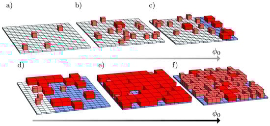
Figure 1.
Schematic representation of a system composed of molecules present in two states: small (S, light red cubes) and large (L, dark red cuboids). From diagrams (a–f): illustration of how the system may phase-separate upon increasing . The phases, here colored in white and blue, can assume different sizes and compositions depending on the values of , , , and . The gray arrows below the diagrams indicate the increase in , with darker gray for larger . Results illustrate a two-dimensional lattice for .
The Helmholtz free energy of the system, , is composed of an entropic contribution, ; energy terms related to switching particles between their L-state and S-state, ; and interactions of particles with solvent molecules, . The absolute temperature is denoted by T and the configurational entropy by S. A lattice–sublattice approximation proposed by Han and co-workers [43] allows us to estimate S as
where denotes the Boltzmann constant. The energy contribution is a single-particle energy that can be written as , where quantifies the energy penalty required for a single molecule to switch from the L-state to the S-state. Finally, the particle–solvent interactions, per lattice site, are accounted for on the mean-field level by the expression
where characterizes the interaction strength between a lattice site occupied by a solvent molecule and a lattice site occupied by a particle. Our definition of the particle–solvent interaction effectively amounts to introducing a tension between the particles and the solvent. Positive tension favors not only the aggregation of particles but also the S-state over the L-state of isolated particles that are surrounded by solvent. Note that both and are dimensionless. For the sake of mathematical simplicity, Equation (2) is based on the assumption that solvent molecules interact with particles in the S-state and L-state in the same way, and S particles and L particles do not interact with each other. In a more general approach, one would assign distinct interaction strengths to pairs of L particles and solvent, S particles and solvent, and L particles and S particles. With the energy contributions specified above, the (dimensionless) free energy per lattice site, , reads
To analyze how the interaction strengths and affect the number of particles residing in their S-state and L-state, we must first obtain the equilibrium distributions. To this end, we insert the relation into Equation (3) and find the global minimum of as a function of . That is, we solve
for , and from all solutions we select that of the lowest energy to obtain the optimal (equilibrium) distribution for fixed and any set of parameters . Hence, the optimal value of the free energy, minimized for the number of L particles versus S particles, reads
Known affords the calculation of phase separation via the familiar common-tangent construction [44].
3. Results and Discussion
We start our discussion by presenting in Figure 2 a series of diagrams that illustrate how the free energy and optimal distributions of states are calculated for a given set of , and ; in this particular case, we chose , , and . As mentioned above, the optimal value is determined such that the free energy adopts a global minimum. Diagrams (a) and (b) of Figure 2 display as a function of for and , respectively, with the global minimum being marked by a blue bullet in each case.
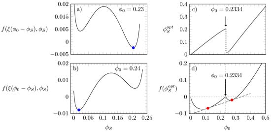
Figure 2.
Diagrams (a,b): free energy according to Equation (3), calculated as a function of for and ; blue bullets mark the global minimum. Diagram (c): as a function of . Diagram (d): as a function of with red bullets marking the points that connect through a common tangent. In all four diagrams, , and .
Upon increasing from to , the position of the global minimum moves from to . Diagram (c) reveals that the distribution of states changes discontinuously at . At this value, the function has two minima with equal depth. Furthermore, as shown in diagram (d) of Figure 2, if we calculate the free energy as a function of , we observe that is the value where adopts a local “cusp-like” maximum, thus necessitating the existence of a common tangent and, hence, two coexisting phases. Indeed, the red bullet diagram (d) in Figure 2 mark the points that exhibit a common tangent (dashed gray line); these correspond to the compositions of the two coexisting phases; each phase with its own value of .
The results shown in Figure 2 correspond to a specific choice of the interaction parameters and . In order to account for other choices, we present in Figure 3 results for and versus for values ranging from to and three different choices of : in diagrams (a) and (b), in diagrams (c) and (d), and in diagrams (e) and (f). Recall that is the solution of Equation (4), thus being the value at which adopts a global minimum. The main diagrams magnify the region , whereas the insets display the results in the range ; all results in Figure 3 are obtained for , and the values are color-coded according to the legends on the side-panels. In diagrams (a) and (b)—top row—we observe that, irrespective of the values of , all distributions of are continuous, and the free energies exhibit a single minimum. For , increasing produces results that evolve from straight lines (purple and blueish curves) to distributions that tend to bend at (red and brown curves). For larger , as in panels (c) and (d), where , the -curves do not only bend but, for some values of , start to display a discontinuity analogous to that observed in Figure 2c. A similar behavior is also present in the bottom row of diagrams, but, as in this case is even larger (), the curves are discontinuous over a wider ranger of values; in both rows of diagrams we gray-shaded the area where the initial growth of is followed by a discontinuous jump to smaller values, and color-matching dotted lines are plotted as a visual guide for this change. For larger , the free energy displays two minima, which become more pronounced upon increasing ; for example, for , the larger the values of , the closer the minima to and to .
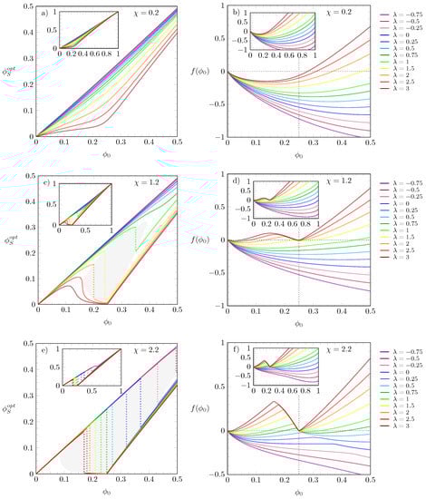
Figure 3.
Left and right diagrams display the values of and , respectively, versus for different and fixed . Each row corresponds to a specific value of : (top), (middle), and (bottom). In all diagrams, the values of are color-coded according to the side legend on the right. The values are solutions of Equation (4), i.e., the value of that globally minimizes the free energy . The shaded gray areas mark the region where the values change discontinuously, and the color-matching dotted lines indicate discontinuity of . Insets display the results over the entire range .
The limit of small offers a transparent discussion of the different roles that and play for the particles to reside in the S-state or L-state; recall that is the energy cost required to switch a single particle from its large (L) to its small (S) size [7] and that accounts for the effective surface tension (a line tension in the two-dimensional case) that acts on the particles when in contact with the solvent.
Upon increasing , starting from , the lattice becomes populated with particles either in the L-state or S-state. When is sufficiently large, the surface tension between the particles and the solvent results in the S-state dominating. Growing gives rise to an increasingly large number of particle–particle interactions that replace particle–solvent interactions. For , where the L-state is energetically preferred over the S-state, this may lead to a transition to a dense phase dominated by the L-state. Let us analyze which state, L or S, dominates in the limit of small . To this end, it is useful to calculate the slope of as a function of for fixed and . A linear relation is valid in the limit of small . Assuming in Equation (3) and expanding around , we arrive at the following solution for the slope s:
Results from Equation (6) are plotted in Figure 4 for different values of , color-coded according to the legend. To visualize the predictions of Equation (6), Figure 4 also displays system illustrations for small slopes, where most of the particles are in the L-state (bottom left inset), and another, for large s, where virtually all particles are in the S-state (top right inset). We note that the larger , the more particles reside initially in the S-state. Furthermore, if is also large, the values of tend to be virtually zero right after the discontinuous jump of , as can be seen in orange, red, and brown curves in Figure 3e. Thus, any particle further added to the lattice will readily assume the L-state. This trend, however, does not continue when grows further: for large , more particles in the L-state are placed on the lattice until steric constraints force them to undergo a transition to the smaller S-state.
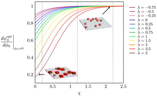
Figure 4.
Slope from the free energy expansion around as a function of the interaction parameter , calculated according to Equation (6). The values of are color-coded according to the side legend. The black dotted lines mark the values used in the diagrams of Figure 3, i.e., , , and . The insets display illustrations of two systems, one with particles mostly in the L-state (bottom left) and another with all particles in the S-state (top right).
In Figure 5, we display phase diagrams for and a different value of for each panel: (a), (b), (c), and (d); as it is common [44,45,46], we present our results in diagrams versus . Note that is proportional to the absolute temperature T because is an interaction energy scaled by the thermal energy unit . In addition to displaying selected tie lines connecting the coexisting phases, the heat map in each panel shows the fraction , with values colored according to the sidebar legend. As we argue in our discussion of Figure 2, changes in have a direct effect on how the free energies vary as a function of . Specifically, discontinuous changes of always imply the presence of a common tangent and thus a phase transition. This is indeed the case in the presented phase diagrams. The critical point, that is, the smallest value of at which for a given a phase transition can occur can be calculated [46,47,48] from solving the three equations
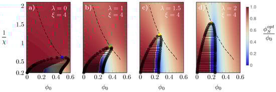
Figure 5.
Phase diagrams, versus , for and different values of : , 1, , and 2 in panels (a–d), respectively. The critical value of is marked by colored bullets: blue (), green (), yellow (), and green (). The dashed line shown in all diagrams is the line on which all critical values lie. The “heat maps” in the background display the value of color-coded according to the side legend.
As our parameter space has five dimensions (), we can use Equation (7) to calculate three critical parameters (, , ) in terms of the other two fixed variables (, ). The critical , here denoted by , is marked by bullets in Figure 5, colored according to the same scheme as in the previous figures. The dashed line—reproduced in all diagrams of Figure 5—is the line on which all the critical points lie as is varied. Upon increasing , the critical and the corresponding are both reduced. Similarly to what was observed in Figure 2, this occurs because the larger the energy cost , the less favorable is the switch. Furthermore, we also observe an evolution of the spinodal line towards a more uniformly convex and symmetric profile. Interestingly, the presence of a concave region of the spinodal line for small suggests the possibility of a single phase-two phases-single phase sequence of phase transitions. In diagram (a) of Figure 5, for example, decreasing the temperature (which corresponds to increasing ) at fixed passes from a single phase to a two-phase region and, subsequently, back to a single phase.
In order to investigate the effects of further increasing , in diagrams (a) and (b) of Figure 6 we show results obtained for and two different choices of : in (a) and in (b). The latter corresponds to the S-state and L-state having the same size, which leads to the same phase diagram as the regular Bragg–Williams free energy. Hence, in diagram (b), the critical point is , and , whereas for diagram (a), the location of the critical point is close to , and . More generally, in the limit of large , where the L-state is enforced, the critical point is located at and . To bridge between these limiting cases, in panel (c) of Figure 6 we display how the critical point and corresponding vary as a function of for different choices of (symbols are color-coded according to the side legend).
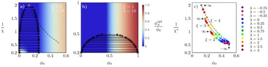
Figure 6.
Phase diagrams for with (a) and (b). The dashed line in (a) is the line along which the critical values of lie; the heat maps in (a) and (b) display the value of , color-coded according to the side legend in (b). Diagram (c): location of critical points, where each set of dashed lines and symbols correspond to , 3, 4, from bottom to top lines; values of are color-coded as specified in the side panel, and the gray bullets mark the limits . For , all critical points merge into one location at and , irrespective of .
The three sets of dashed lines, on which the corresponding symbols lie, were calculated for , 3, and 4, from bottom to top. For each , the gray bullets mark the results obtained in the limit of (bottom right) and (left bullets, as indicated by arrows). In the limit of , the S-state is enforced. Hence, as in this case the system consists exclusively of particles in the S-state, all lines converge to the Bragg–Williams result irrespective of the value of . In the opposite limit, i.e., , all particles adopt the L-state. Consequently, the system behaves as composed solely of particles in the L-state, with particle volume , and we obtain the familiar Bragg–Williams result, but for a lattice with times larger lattice sites. As is close to the limit , the mechanism above provides a rationale for the findings in diagrams (a) and (b).
We finally note that the function can be used to calculate [7] the pressure P of the system through
In Figure 7, we present isotherms for the scaled pressure as a function of for three different choices of : (a), (b), and (c). Different values of are color-coded according to the side legend, and all results were obtained for . Because corresponds to effectively attractive interactions between the particles, increasing always reduces P at fixed . Despite this, increasing at fixed does not always increase P, despite the growing preference for the L-state. The pressure tends to increase with for and for if . However, for and , increasing lowers the pressure of a phase-separated system because a larger degree of aggregation is induced that involves a smaller number of particles and, thus, a lower pressure.
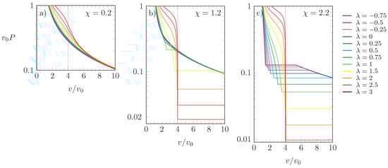
Figure 7.
Scaled pressure versus for (a), (b), and (c). Different colors correspond to different values of , as indicated in the side legend. The dotted line marks the point . Results calculated for .
4. Conclusions and Outlook
Molecules with internal degrees of freedom are ubiquitous in nature. Colloids, proteins, and microgels, are just a few examples of molecules that can adjust their size in response to external stimuli. In the present work, we developed a simple extension of the Bragg–Williams model to describe solvent-immersed particles that can exist in two states, one of a larger (L) and another of a smaller size (S). Our model is based on a lattice–sublattice approximation [7,43] and accounts for particle–solvent interactions on the mean-field level. More specifically, we considered two energy parameters: , the cost of a particle to switch from the L-state to the S-state, and , an effective particle–solvent interaction that acts analogously to a surface tension and is independent of the state in which the particles reside. We focused our analysis on how these parameters affect thermodynamic properties: the distribution of particle states as expressed by and the occurrence of phase separation. Phase diagrams show how the energetic preference of the particles for one or the other state affects phase transitions and compositions of coexisting phases. We also calculated critical points and considered the effect of varying , the size ratio between the particles in their L-state and S-state. In the limit of very large positive or negative values, our model recovers familiar results of the Bragg–Williams model. We designed our model to apply to systems composed of particles that can reside in two states of different size. However, its generalization to particles with more than two size-dependent states is straightforward. Other possible extensions account for interactions between particles in different states as well as distinct interactions between solvent molecules and particles in different states. Finally, our model has the capacity to serve as a tool to rationalize different contributions to experimentally observed “shoulders” in surface pressure–area isotherms [30,39,40] and phase transitions of monolayers [49,50].
Author Contributions
Conceptualization and methodology, G.V.B. and S.M.; validation, G.V.B. and S.M.; investigation, G.V.B. and S.M.; writing—original draft preparation, G.V.B.; writing—review and editing, S.M. All authors have read and agreed to the published version of the manuscript.
Funding
G.V.B. acknowledges support from Vicerrectoría de Investigación, Desarrollo y Creación Artística (VIDCA/UACh) project INS-INV 2022-09. S.M. acknowledges financial support through the Phospholipid Research Center, Heidelberg, Germany (SMA-2018-061/1-1), and support by (while serving at) the National Science Foundation.
Institutional Review Board Statement
Not applicable.
Informed Consent Statement
Not applicable.
Data Availability Statement
Not applicable.
Conflicts of Interest
The authors declare no conflict of interest. The funders had no role in the design of the study; in the collection, analyses, or interpretation of data; in the writing of the manuscript; or in the decision to publish the results.
References
- Baoukina, S.; Monticelli, L.; Marrink, S.J.; Tieleman, D.P. Pressure- area isotherm of a lipid monolayer from molecular dynamics simulations. Langmuir 2007, 23, 12617–12623. [Google Scholar] [CrossRef]
- Blanco, E.; Pineiro, A.; Miller, R.; Ruso, J.M.; Prieto, G.; Sarmiento, F. Langmuir monolayers of a hydrogenated/fluorinated catanionic surfactant: From the macroscopic to the nanoscopic size scale. Langmuir 2009, 25, 8075–8082. [Google Scholar] [CrossRef] [PubMed]
- Javanainen, M.; Lamberg, A.; Cwiklik, L.; Vattulainen, I.; Ollila, O.S. Atomistic model for nearly quantitative simulations of Langmuir monolayers. Langmuir 2018, 34, 2565–2572. [Google Scholar] [CrossRef] [PubMed]
- Ermakov, Y.A.; Asadchikov, V.; Roschin, B.; Volkov, Y.O.; Khomich, D.; Nesterenko, A.; Tikhonov, A. Comprehensive study of the liquid expanded–liquid condensed phase transition in 1, 2-dimyristoyl-sn-glycero-3-phospho-L-serine monolayers: Surface pressure, Volta potential, X-ray reflectivity, and molecular dynamics modeling. Langmuir 2019, 35, 12326–12338. [Google Scholar] [CrossRef] [PubMed]
- Linse, P.; Bjoerling, M. Lattice theory for multicomponent mixtures of copolymers with internal degrees of freedom in heterogeneous systems. Macromolecules 1991, 24, 6700–6711. [Google Scholar] [CrossRef]
- Karnieli, A.; Markovich, T.; Andelman, D. Surface pressure of charged colloids at the air/water interface. Langmuir 2018, 34, 13322–13332. [Google Scholar] [CrossRef]
- Agudelo, J.; Bossa, G.V.; May, S. Incorporation of Molecular Reorientation into Modeling Surface Pressure-Area Isotherms of Langmuir Monolayers. Molecules 2021, 26, 4372. [Google Scholar] [CrossRef]
- Walter, J.; Sehrt, J.; Vrabec, J.; Hasse, H. Molecular dynamics and experimental study of conformation change of poly (N-isopropylacrylamide) hydrogels in mixtures of water and methanol. J. Phys. Chem. B 2012, 116, 5251–5259. [Google Scholar] [CrossRef]
- Culver, H.R.; Clegg, J.R.; Peppas, N.A. Analyte-responsive hydrogels: Intelligent materials for biosensing and drug delivery. Acc. Chem. Res. 2017, 50, 170–178. [Google Scholar] [CrossRef]
- Cilla, S.; Floría, L. Internal degrees of freedom in a thermodynamical model for intracell biological transport. Phys. D 1998, 113, 157–161. [Google Scholar] [CrossRef]
- Guigas, G.; Weiss, M. Size-dependent diffusion of membrane inclusions. Biophys. J. 2006, 91, 2393–2398. [Google Scholar] [CrossRef]
- Ilie, I.M.; den Otter, W.K.; Briels, W.J. A coarse grained protein model with internal degrees of freedom. Application to α-synuclein aggregation. J. Chem. Phys. 2016, 144, 085103. [Google Scholar] [CrossRef] [PubMed]
- Kumaki, J.; Hashimoto, T. Conformational change in an isolated single synthetic polymer chain on a mica surface observed by atomic force microscopy. J. Am. Chem. Soc. 2003, 125, 4907–4917. [Google Scholar] [CrossRef] [PubMed]
- Shen, X.; Viney, C.; Johnson, E.R.; Wang, C.; Lu, J.Q. Large negative thermal expansion of a polymer driven by a submolecular conformational change. Nat. Chem. 2013, 5, 1035–1041. [Google Scholar] [CrossRef] [PubMed]
- Yefimov, S.; Van der Giessen, E.; Onck, P.R.; Marrink, S.J. Mechanosensitive membrane channels in action. Biophys. J. 2008, 94, 2994–3002. [Google Scholar] [CrossRef] [PubMed]
- Rasmussen, T.; Flegler, V.J.; Rasmussen, A.; Böttcher, B. Structure of the mechanosensitive channel MscS embedded in the membrane bilayer. J. Mol. Biol. 2019, 431, 3081–3090. [Google Scholar] [CrossRef]
- Zhang, Y.; Daday, C.; Gu, R.X.; Cox, C.D.; Martinac, B.; de Groot, B.L.; Walz, T. Visualization of the mechanosensitive ion channel MscS under membrane tension. Nature 2021, 590, 509–514. [Google Scholar] [CrossRef]
- Thorne, J.B.; Vine, G.J.; Snowden, M.J. Microgel applications and commercial considerations. Colloid Polym. Sci. 2011, 289, 625–646. [Google Scholar] [CrossRef]
- Urich, M.; Denton, A.R. Swelling, structure, and phase stability of compressible microgels. Soft Matter 2016, 12, 9086–9094. [Google Scholar] [CrossRef]
- Marcisz, K.; Mackiewicz, M.; Romanski, J.; Stojek, Z.; Karbarz, M. Significant, reversible change in microgel size using electrochemically induced volume phase transition. Appl. Mater. Today 2018, 13, 182–189. [Google Scholar] [CrossRef]
- Butler, M.D.; Montenegro-Johnson, T.D. The swelling and shrinking of spherical thermo-responsive hydrogels. J. Fluid Mech. 2022, 947, A11. [Google Scholar] [CrossRef]
- Reese, C.E.; Mikhonin, A.V.; Kamenjicki, M.; Tikhonov, A.; Asher, S.A. Nanogel nanosecond photonic crystal optical switching. J. Am. Chem. Soc. 2004, 126, 1493–1496. [Google Scholar] [CrossRef] [PubMed]
- Giner-Casares, J.J.; Brezesinski, G.; Möhwald, H. Langmuir monolayers as unique physical models. Curr. Opin. Colloid Interface Sci. 2014, 19, 176–182. [Google Scholar] [CrossRef]
- Stefaniu, C.; Brezesinski, G.; Möhwald, H. Langmuir monolayers as models to study processes at membrane surfaces. Adv. Colloid Interface Sci. 2014, 208, 197–213. [Google Scholar] [CrossRef] [PubMed]
- Oliveira, O.N., Jr.; Caseli, L.; Ariga, K. The past and the future of Langmuir and Langmuir–Blodgett films. Chem. Rev. 2022, 122, 6459–6513. [Google Scholar] [CrossRef] [PubMed]
- McConnell, H.M.; Radhakrishnan, A. Condensed complexes of cholesterol and phospholipids. Biochim. Biophys. Acta Biomembr. 2003, 1610, 159–173. [Google Scholar] [CrossRef]
- Jurak, M. Thermodynamic aspects of cholesterol effect on properties of phospholipid monolayers: Langmuir and Langmuir–Blodgett monolayer study. J. Phys. Chem. B 2013, 117, 3496–3502. [Google Scholar] [CrossRef]
- Janich, C.; Hädicke, A.; Bakowsky, U.; Brezesinski, G.; Wölk, C. Interaction of DNA with Cationic Lipid Mixtures: Investigation at Langmuir Lipid Monolayers. Langmuir 2017, 33, 10172–10183. [Google Scholar] [CrossRef]
- Luque-Caballero, G.; Maldonado-Valderrama, J.; Quesada-Pérez, M.; Martín-Molina, A. Interaction of DNA with likely-charged lipid monolayers: An experimental study. Colloids Surf. B 2019, 178, 170–176. [Google Scholar] [CrossRef]
- Nobre, T.M.; Pavinatto, F.J.; Caseli, L.; Barros-Timmons, A.; Dynarowicz-Łątka, P.; Oliveira, O.N., Jr. Interactions of bioactive molecules & nanomaterials with Langmuir monolayers as cell membrane models. Thin Solid Films 2015, 593, 158–188. [Google Scholar]
- Rojewska, M.; Smułek, W.; Kaczorek, E.; Prochaska, K. Langmuir Monolayer Techniques for the Investigation of Model Bacterial Membranes and Antibiotic Biodegradation Mechanisms. Membranes 2021, 11, 707. [Google Scholar] [CrossRef]
- Salay, L.C.; Ferreira, M.; Oliveira, O.N., Jr.; Nakaie, C.R.; Schreier, S. Headgroup specificity for the interaction of the antimicrobial peptide tritrpticin with phospholipid Langmuir monolayers. Colloids Surf. B 2012, 100, 95–102. [Google Scholar] [CrossRef]
- Martynowycz, M.W.; Rice, A.; Andreev, K.; Nobre, T.M.; Kuzmenko, I.; Wereszczynski, J.; Gidalevitz, D. Salmonella membrane structural remodeling increases resistance to antimicrobial peptide LL-37. ACS Infect. Dis. 2019, 5, 1214–1222. [Google Scholar] [CrossRef] [PubMed]
- Fainerman, V.; Vollhardt, D. Surface pressure isotherm for the fluid state of Langmuir monolayers. J. Phys. Chem. B 2006, 110, 10436–10440. [Google Scholar] [CrossRef] [PubMed]
- Klug, J.; Masone, D.; Del Pópolo, M.G. Molecular-level insight into the binding of arginine to a zwitterionic Langmuir monolayer. RSC Adv. 2017, 7, 30862–30869. [Google Scholar] [CrossRef]
- Levental, I.; Janmey, P.; Cēbers, A. Electrostatic contribution to the surface pressure of charged monolayers containing polyphosphoinositides. Biophys. J. 2008, 95, 1199–1205. [Google Scholar] [CrossRef]
- Chachaj-Brekiesz, A.; Kobierski, J.; Wnętrzak, A.; Dynarowicz-Łatka, P. Electrical properties of membrane phospholipids in Langmuir monolayers. Membranes 2021, 11, 53. [Google Scholar] [CrossRef]
- Miñones, J.; Yebra-Pimentel, E.; Iribarnegaray, E.; Conde, O.; Casas, M. Compression—expansion curves of cyclosporin A monolayers on substrates of various ionic strengths. Colloids Surf. A 1993, 76, 227–232. [Google Scholar] [CrossRef]
- Hąc-Wydro, K.; Dynarowicz-Łątka, P. Nystatin in Langmuir monolayers at the air/water interface. Colloids Surf. B 2006, 53, 64–71. [Google Scholar] [CrossRef] [PubMed]
- Wnętrzak, A.; Chachaj-Brekiesz, A.; Janikowska-Sagan, M.; Rodriguez, J.L.F.; Conde, J.M.; Dynarowicz-Łatka, P. Crucial role of the hydroxyl group orientation in Langmuir monolayers organization–The case of 7-hydroxycholesterol epimers. Colloids Surf. A 2019, 563, 330–339. [Google Scholar] [CrossRef]
- Strzalka, J.; Chen, X.; Moser, C.C.; Dutton, P.L.; Ocko, B.M.; Blasie, J.K. X-ray scattering studies of maquette peptide monolayers. 1. Reflectivity and grazing incidence diffraction at the air/water interface. Langmuir 2000, 16, 10404–10418. [Google Scholar] [CrossRef]
- Davis, H.T. Statistical Mechanics of Phases, Interfaces, and Thin Films; Wiley: Hoboken, NJ, USA, 1996. [Google Scholar]
- Han, Y.; Huang, S.; Yan, T. A mean-field theory on the differential capacitance of asymmetric ionic liquid electrolytes. J. Phys. Condens. Matter 2014, 26, 284103. [Google Scholar] [CrossRef] [PubMed]
- Jones, R.A. Soft Condensed Matter; Oxford University Press: Oxford, UK, 2002; Volume 6. [Google Scholar]
- Andelman, D.; Brochard, F.; Knobler, C.; Rondelez, F. Structures and phase transitions in Langmuir monolayers. In Micelles, Membranes, Microemulsions and Monolayers; Springer: New York, NY, USA, 1994; pp. 559–602. [Google Scholar]
- Bossa, G.V.; Gunderson, S.; Downing, R.; May, S. Role of transmembrane proteins for phase separation and domain registration in asymmetric lipid bilayers. Biomolecules 2019, 9, 303. [Google Scholar] [CrossRef] [PubMed]
- Akasaka, R. Calculation of the critical point for mixtures using mixture models based on Helmholtz energy equations of state. Fluid Phase Equilib. 2008, 263, 102–108. [Google Scholar] [CrossRef]
- Bell, I.H.; Jäger, A. Calculation of critical points from Helmholtz-energy-explicit mixture models. Fluid Phase Equilib. 2017, 433, 159–173. [Google Scholar] [CrossRef]
- Knobler, C.M.; Desai, R.C. Phase transitions in monolayers. Annu. Rev. Phys. Chem. 1992, 43, 207–236. [Google Scholar] [CrossRef]
- Dynarowicz-Łatka, P.; Dhanabalan, A.; Oliveira, O.N. A study on two-dimensional phase transitions in langmuir monolayers of a carboxylic acid with a symmetrical triphenylbenzene ring system. J. Phys. Chem. B 1999, 103, 5992–6000. [Google Scholar] [CrossRef]
Disclaimer/Publisher’s Note: The statements, opinions and data contained in all publications are solely those of the individual author(s) and contributor(s) and not of MDPI and/or the editor(s). MDPI and/or the editor(s) disclaim responsibility for any injury to people or property resulting from any ideas, methods, instructions or products referred to in the content. |
© 2023 by the authors. Licensee MDPI, Basel, Switzerland. This article is an open access article distributed under the terms and conditions of the Creative Commons Attribution (CC BY) license (https://creativecommons.org/licenses/by/4.0/).