Article

The Expected Values for the Gutman Index and Schultz Index in the Random Regular Polygonal Chains

School of Mathematics and Big Data, Anhui University of Science & Technology, Huainan 232000, China
*
Author to whom correspondence should be addressed.
Molecules 2022, 27(20), 6838; https://doi.org/10.3390/molecules27206838
Submission received: 23 September 2022 / Revised: 8 October 2022 / Accepted: 10 October 2022 / Published: 12 October 2022
(This article belongs to the Special Issue Study of Molecules in the Light of Spectral Graph Theory)

Abstract

:
Two famous topological indices, the Gutman index and Schultz index, are studied in this article. We mainly calculate the exact analytical formulae for the expected values of the Gutman index and Schultz index of a random regular polygonal chain with n regular polygons. Moreover, we determine the average values and the extremal values of the indices in regard to the set of all these regular polygonal chains.

1. Introduction

Thus far, chemistry has been extensively studied and applied in graph theory [1,2,3,4]. It is often the case that chemical compounds can be interpreted by chemical graphs, in which vertices represent the atoms and edges stand for the covalent bonds between atoms. The random regular polygonal chains studied here are obtained by randomly connecting n regular polygons through vertex-to-vertex in turn; these connection vertices are termed cut vertex. Meanwhile, the random regular polygonal chains with n regular polygons are spiro compounds, which are a significant class of cycloalkanes in organic chemistry; refer to [5,6]. Spiro compounds have a rigid and stable structure, their chiral ligands have a large specific optical rotation, and they have important applications in asymmetric catalysis, luminescent materials, pesticides, polymer binders and so on.
In theoretical chemistry, topological indices are commonly used to encode molecules, as well as to design compounds with physicochemical properties or biological activity [7]. It is a popular issue to study the topological indices of the chemical chains and their significance.
Throughout this paper, all the graphs that we take into account are finite, undirected and simple; a graph is simple if it has no loops and no two of its links join the same pair of vertices. More detailed notations and terminologies can be found in [8]. Let G = ( V ( G ) , E ( G ) ) be a disordered graph; V ( G ) represents the vertex set and E ( G ) stands for the edge set. The degree d G ( u ) , or d ( u ) for short, is the number of edges connected to the node u( u V ( G ) ). The length of the shortest path between vertex u and vertex v( u , v V ( G ) ) is defined as the distance d G ( u , v ) (short for d ( u , v ) ). The sum of the distances between any two vertices in V ( G ) is d ( u | G ) = v V ( G ) d ( u , v ) .
The Wiener index [9,10,11,12,13,14] is the best-known of all topological indices, which is defined as W ( G ) = { u , v } V ( G ) d G ( u , v ) . By weighting the Wiener index, the Gutman index is proposed as
G u t ( G ) = 1 2 u V G v V G ( d G ( u ) d G ( v ) ) d G ( u , v ) = { u , v } V ( G ) ( d G ( u ) d G ( v ) ) d G ( u , v ) ,
which is a kind of vertex-valency-weighted sum of the distance between all pairs of vertices in a graph [15,16,17,18,19]. The index is closely related to the Wiener index and has the same structured features as the Wiener index in the condition of acyclic structures. Therefore, the research for the possible chemical applications of the Gutman index and the theoretical investigations should lay particular emphasis on the condition of polycyclic molecules.
The Schultz index [20] is proposed as
S ( G ) = 1 2 u V G v V G ( d G ( u ) + d G ( v ) ) d G ( u , v ) = { u , v } V ( G ) ( d G ( u ) + d G ( v ) ) d G ( u , v ) .
The Schultz index has been shown to be a useful molecular descriptor in the design of molecules with desired properties [21]; thus, further studies on the mathematical and computational properties of the Schultz index are desirable, including more articles on developing such topology indices of the mathematical properties and applications [22].
Many scholars have studied the indices of some random polyphenylene chains before [23,24,25,26,27,28]. Recently, Liu and Zeng et al. [29] obtained some indices in the random spiro chains, including the Gutman index, Schultz index, multiplicative-degree Kirchhoff index and additive-degree Kirchhoff index, and determined the expected values of these indices in the random spiro chain, and the extremal values among all spiro chain with n hexagons. Motivated by [29,30,31], we explore the property of the Gutman index and Schultz index of polygonal regular chains, and determine the expected values of the indices, denoted by E ( G u t ( S C n ) ) and E ( S ( S C n ) ) in the random regular polygonal chains with n regular polygons, and we discuss the maximum and minimum of the E ( G u t ( S C n ) ) and E ( S ( S C n ) ) . Meanwhile, we acquire the extremal values and the average values of the Gutman index and Schultz index among all regular polygonal chains with n regular polygons.
The random regular polygonal chain S C n + 1 with n + 1 regular polygons consists of a new regular polygon G n + 1 attaching to the end of a regular polygonal chain S C n with n regular polygons; see Figure 1.
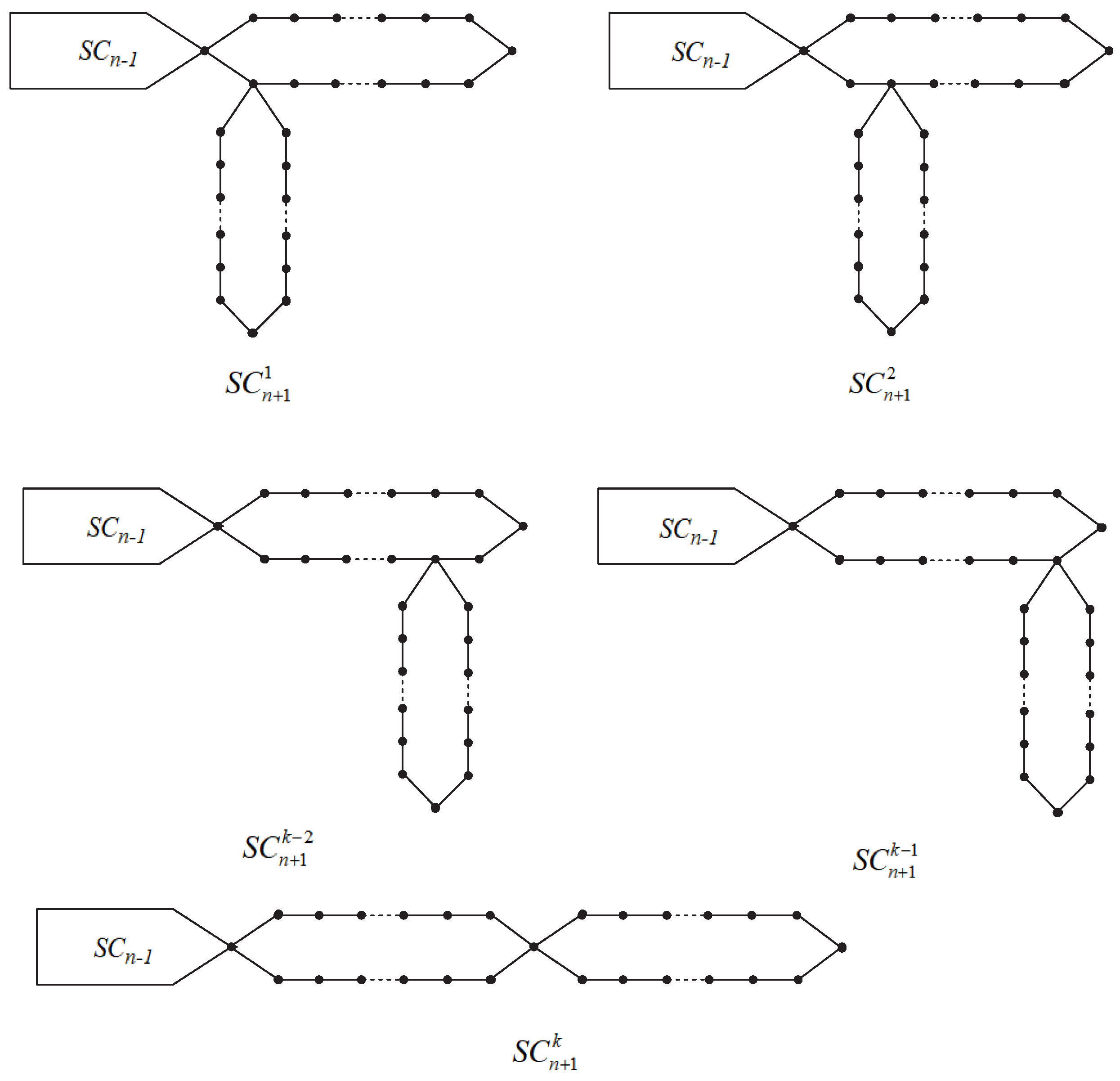
For n 3 , there are k ways to connect the terminal regular polygon G n + 1 with the front random regular polygonal chain S C n . They can be described as S C n + 1 1 , S C n + 1 2 , , S C n + 1 k 1 and S C n + 1 k , respectively; see Figure 2.
A random regular polygonal chain S C n with n regular polygons can be obtained by adding a regular polygon at the end of the chain step by step. At each step t ( = 3 , 4 , , n ) , a random connection is made from one of the following k possible cases:
  • S C t S C t + 1 1 with probability p 1 ,
  • S C t S C t + 1 2 with probability p 2 ,
  • S C t S C t + 1 3 with probability p 3 ,
  • S C t S C t + 1 k with probability p k = 1 ( p 1 + p 2 + p 3 + + p k 1 ) ,
where the k probabilities p 1 , p 2 , , p k 1 and p k are independent of the step parameter t. When p 1 = 1 , p 2 = p 3 = = p k = 0 , the meta-chain M n can be obtained. When p 2 = 1 , p 1 = p 3 = = p k = 0 , the orth-chain O n 1 can be obtained. When p 3 = 1 , p 1 = p 2 = p 4 = = p k = 0 , the orth-chain O n 2 can be obtained. When p k 1 = 1 , the other k 1 probabilities reach 0, and we can obtain the orth-chain O n k 2 . When p k = 1 , p 1 = p 2 = = p k 1 = 0 , the para-chain P n can be obtained.

2. The Gutman Index of the Random Regular Polygonal Chain

For the random regular polygonal chain S C n , we denote by S C n + 1 the graph acquired by connecting a new terminal regular polygon G n + 1 to S C n , which is spanned by vertices x 1 , x 2 , , x 2 k and x 1 is u n (see Figure 1). It is evident that, for all v S C n , we have
d ( v , x j ) = d ( v , u n ) + j 1 , 1 j k d ( v , u n ) + 2 k + 1 j , k + 1 j 2 k .
v V ( S C n ) d S C n + 1 ( v ) = 4 k n + 2 .
Meanwhile, we obtain that
i = 1 2 k d ( x i ) d ( x i , x j ) = 2 k 2 + 2 ( j 1 ) , 1 j k 2 k 2 + 2 ( 2 k j + 1 ) , k + 1 j 2 k .
Theorem 1.
The E [ G u t ( S C n ) ] ( n 1 ) of the random regular polygonal chain is
E [ G u t ( S C n ) ] = 8 3 k 2 n 3 [ k i = 1 k 1 ( k i ) p i ] + 8 k 2 n 2 [ i = 1 k 1 ( k i ) p i ] + 4 3 k 2 n [ k 4 i = 1 k 1 ( k i ) p i ] .
Proof. 
Let G u t ( S C n ) = A 1 + B 1 + C 1 .
A 1 = { u , v } S C n d ( u ) d ( v ) d ( u , v ) , = { u , v } S C n { u n } d ( u ) d ( v ) d ( u , v ) + v S C n { u n } d S C n + 1 ( u n ) d ( v ) d ( u n , v ) , = { u , v } S C n { u n } d ( u ) d ( v ) d ( u , v ) + v S C n { u n } [ d S C n ( u n ) + 2 ] d ( v ) d ( u n , v ) , = G u t ( S C n ) + 2 v S C n d ( v ) d ( u n , v ) . B 1 = v S C n { u n } x i G n + 1 { x 1 } d ( v ) d ( x i ) d ( v , x i ) , = v S C n x i G n d ( v ) d ( x i ) d ( v , x i ) 4 v S C n d ( v ) d ( v , u n ) 4 v G n + 1 d ( v ) d ( v , x 1 ) , = v S C n d ( v ) { 4 d ( v , u n ) + 4 [ d ( v , u n ) + 1 ] + 4 [ d ( v , u n ) + 2 ] + + 4 [ d ( v , u n ) + k 1 ] + 2 [ d ( v , u n ) + k ] } , 4 v S C n d ( v ) d ( v , u n ) 4 × 2 k 2 , = ( 4 k 2 ) v S C n d ( v ) d ( v , u n ) + 2 k 2 ( 4 k n 2 ) . C 1 = { x i , x j } G n + 1 d ( x i ) d ( x j ) d ( x i , x j ) , = 1 2 i = 1 2 k d ( x i ) ( j = 1 2 k d ( x j ) d ( x j , x i ) ) , = 4 k 2 ( k + 1 ) .
Then, G u t ( S C n + 1 ) = G u t ( S C n ) + 4 k v S C n d ( v ) d ( v , u n ) + 8 k 3 n + 4 k 3 .
For convenience, we could denote the random variable v S C n d ( v ) d ( v , u n ) by
U n 1 : = E ( v S C n d ( v ) d ( v , u n ) ) .
Therefore, we can obtain a recurrence relation as follows:
E ( G u t ( S C n + 1 ) ) = E ( G u t ( S C n ) ) + 4 k U n 1 + 8 k 3 n + 4 k 3 .
By considering the following k possible conditions, it is easy to obtain U n 1 .
Condition 1.
S C n S C n + 1 1 , then u n would cover the vertex x 2 or x 2 k . Hence, v V S C n d ( u n , v ) can be represented as v V S C n d ( x 2 , v ) or v V S C n d ( x 2 k , v ) with probability p 1 .
Condition 2.
S C n S C n + 1 2 , then u n would cover the vertex x 3 or x 2 k 1 . Hence, v V S C n d ( u n , v ) can be represented as v V S C n d ( x 3 , v ) or v V S C n d ( x 2 k 1 , v ) with probability p 2 .
Condition 3.
S C n S C n + 1 k 2 , then u n would cover the vertex x k 1 or x k + 3 . Hence, v V S C n d ( u n , v ) can be represented as v V S C n d ( x k 1 , v ) or v V S C n d ( x k + 3 , v ) with probability p k 2 .
Condition 4.
S C n S C n + 1 k 1 , then u n would cover the vertex x k or x k + 2 . Hence, v V S C n d ( u n , v ) can be represented as v V S C n d ( x k , v ) or v V S C n d ( x k + 2 , v ) with probability p k 1 .
Condition 5.
S C n S C n + 1 k , then u n would cover the vertex x k + 1 . Hence, v V S C n d ( u n , v ) can be represented as v V S C n d ( x k + 1 , v ) with probability 1 p 1 p 2 p k 1 .
According to the k conditions, we have that
U n 1 = p 1 v S C n d ( v ) d ( v , x 2 ) + p 2 v S C n d ( v ) d ( v , x 3 ) + + p k 1 v S C n d ( v ) d ( v , x k ) + ( 1 p 1 p 2 p k 1 ) v S P C n d ( v ) d ( v , x k + 1 ) , = p 1 [ v S C n 1 d ( v ) d ( v , u n 1 ) + v S C n 1 { u n 1 } d ( v ) + 2 k 2 + 2 ] + p 2 [ v S C n 1 d ( v ) d ( v , u n 1 ) + 2 v S C n 1 { u n 1 } d ( v ) + 2 k 2 + 4 ] + + p k 1 [ v S C n 1 d ( v ) d ( v , u n 1 ) + ( k 1 ) v S C n 1 { u n 1 } d ( v ) + 2 k 2 + 2 ( k 1 ) ] + ( 1 p 1 p 2 p k 1 ) [ v S C n 1 d ( v ) d ( v , u n 1 ) + k v S C n 1 { u n 1 } d ( v ) + 2 k 2 + 2 k ] ,
= p 1 [ v S C n 1 d ( v ) d ( v , u n 1 ) + 4 k ( n 1 ) + 2 k 2 ] + p 2 [ v S C n 1 d ( v ) d ( v , u n 1 ) + 2 · 4 k ( n 1 ) + 2 k 2 ] + + p k 1 [ v S C n 1 d ( v ) d ( v , u n 1 ) + ( k 1 ) · 4 k ( n 1 ) + 2 k 2 ] + ( 1 p 1 p 2 p k 1 ) [ v S C n 1 d ( v ) d ( v , u n 1 ) + k · 4 k ( n 1 ) + 2 k 2 ] , = U n 1 1 + [ 4 k 2 ( k 1 ) · 4 k p 1 ( k 2 ) · 4 k p 2 4 k p k 1 ] n + [ 2 k 2 + ( k 1 ) · 4 k p 1 + ( k 2 ) · 4 k p 2 + + 4 k p k 1 ] , = U n 1 1 + [ 4 k 2 4 k i = 1 k 1 ( k i ) p i ] n + [ 2 k 2 + 4 k i = 1 k 1 ( k i ) p i ] .
Moreover, the original value is U 1 1 = v S C 1 d ( v ) d ( v , u 1 ) = 2 k 2 . Thus,
U n 1 = [ 2 k 2 2 k i = 1 k 1 ( k i ) p i ] n 2 + [ 2 k i = 1 k 1 ( k i ) p i ] n .
Due to
E ( G u t ( S C n + 1 ) ) = E ( G u t ( S C n ) ) + 4 k U n 1 + 8 k 3 n + 4 k 3 , = E ( G u t ( S P C n ) ) + 8 k 2 n 2 [ k ( k 1 ) p 1 ( k 2 ) p 2 p k 1 ] , + 8 k 2 n [ k + ( k 1 ) p 1 + ( k 2 ) p 2 + + p k 1 ] + 4 k 3 , = E ( G u t ( S P C n ) ) + 8 k 2 n 2 [ k i = 1 k 1 ( k i ) p i ] + 8 k 2 n [ k + i = 1 k 1 ( k i ) p i ] + 4 k 3 .
From the original value, E ( G u t ( S C 1 ) ) = 2 × 2 × 2 k × 1 2 × [ 1 × 2 + 2 × 2 + + 2 × ( k 1 ) + k ] = 4 k 3 , and the above recurrence relation, we may calculate that
E ( G u t ( S C n ) ) = E ( G u t ( S C n ) ) = 8 3 k 2 n 3 [ k ( k 1 ) p 1 ( k 2 ) p 2 p k 1 ] + 8 k 2 n 2 [ ( k 1 ) p 1 + ( k 2 ) p 2 + + p k 1 ] + 4 3 k 2 n [ k 4 ( k 1 ) p 1 4 ( k 2 ) p 2 4 p k 1 ] , = 8 3 k 2 n 3 [ k i = 1 k 1 ( k i ) p i ] + 8 k 2 n 2 [ i = 1 k 1 ( k i ) p i ] + 4 3 k 2 n [ k 4 i = 1 k 1 ( k i ) p i ] .
The proof is complete. □
According to the proof of Theorem 1, if p 1 = 1 , each of the other k 1 probabilities is equal to 0, and then we have S C n M n . Likewise, if p 2 = 1 , each of the other k 1 probabilities is equal to 0, and then S C n O n 1 ; if p 3 = 1 , each of the other k 1 probabilities is equal to 0, and then S C n O n 2 and so on; if p k 1 = 1 , each of the other k 1 probabilities is equal to 0, and then S C n O n k 2 ; if p k = 1 , each of the other k 1 probabilities is equal to 0, and then S C n P n .
Corollary 1.
The Gutman indices of M n , O n 1 , O n 2 , , O n k 2 , P n are
G u t ( M n ) = 8 3 k 2 n 3 + 8 k 2 ( k 1 ) n 2 + 4 3 k 2 ( 4 3 k ) n ;
G u t ( O n 1 ) = 2 · 8 3 k 2 n 3 + 8 k 2 ( k 2 ) n 2 + 4 3 ( 8 3 k ) k 2 n ;
G u t ( O n 2 ) = 3 · 8 3 k 2 n 3 + 8 k 2 ( k 3 ) n 2 + 4 3 ( 12 3 k ) k 2 n ;
G u t ( O n k 2 ) = ( k 1 ) · 8 3 k 2 n 3 + 8 k 2 n 2 + 4 3 [ ( k 1 ) · 4 3 k ] k 2 n ;
G u t ( P n ) = 8 3 k 3 n 3 + 4 3 k 3 n .
Corollary 2.
Among all polygonal chains with n ( n 3 ) 2k polygons, P n realizes the maximum of E ( G u t ( S C n ) ) and M n realizes the minimum of E ( G u t ( S C n ) ) .
Proof. 
By Theorem 1, we have
f 1 = E ( G u t ( S C n ) ) , = [ 8 3 k 2 ( k 1 ) n 3 + 8 k 2 ( k 1 ) n 2 16 3 k 2 ( k 1 ) n ] p 1 + [ 8 3 k 2 ( k 2 ) n 3 + 8 k 2 ( k 2 ) n 2 16 3 k 2 ( k 2 ) n ] p 2 + + [ 8 3 k 2 n 3 + 8 k 2 n 2 16 3 k 2 n ] p k 1 + ( 8 3 k 3 n 3 + 4 3 k 3 n ) .
as n 3 , we have that
f 1 p 1 = 8 3 k 2 ( k 1 ) n 3 + 8 k 2 ( k 1 ) n 2 16 3 k 2 ( k 1 ) n < 0 ;
f 1 p 2 = 8 3 k 2 ( k 2 ) n 3 + 8 k 2 ( k 2 ) n 2 16 3 k 2 ( k 2 ) n < 0 ;
f 1 p k 1 = 8 3 k 2 n 3 + 8 k 2 n 2 16 3 k 2 n < 0 .
When ( p 1 , p 2 , , p k 1 , p k ) = ( 0 , 0 , , 0 , 1 ) , P n realizes the maximum of E [ G u t ( S C n ) ] , thus, S C n P n . If p k = 0 , p 1 + p 2 + + p k 1 = 1 , we can translate this into p k 1 = 1 p 1 p 2 p k 2 ( 0 p l 1 , l [ 1 , k 2 ] ) , then
E [ G u t ( S C n ) ] = [ 8 3 k 2 ( k 1 ) n 3 + 8 k 2 ( k 1 ) n 2 16 3 k 2 ( k 1 ) n ] p 1 + [ 8 3 k 2 ( k 2 ) n 3 + 8 k 2 ( k 2 ) n 2 16 3 k 2 ( k 2 ) n ] p 2 + + [ 8 3 k 2 n 3 + 8 k 2 n 2 16 3 k 2 n ] ( 1 p 1 p 2 p k 2 ) + ( 8 3 k 3 n 3 + 4 3 k 3 n ) .
Thus,
E ( G u t ( S C n ) ) p 1 = 8 3 k 2 ( k 2 ) n 3 + 8 k 2 ( k 2 ) n 2 16 3 k 2 ( k 2 ) n < 0 , E ( G u t ( S C n ) ) p 2 = 8 3 k 2 ( k 3 ) n 3 + 8 k 2 ( k 3 ) n 2 16 3 k 2 ( k 3 ) n < 0 ,
E ( G u t ( S C n ) ) p k 2 = 8 3 k 2 n 3 + 8 k 2 n 2 16 3 k 2 n < 0 .
However, p 1 = p 2 = = p k 2 = 0 (i.e., p k 1 = 1 ), and we cannot acquire the minimum value of E ( G u t ( S C n ) ) . Thus, we consider p 1 + p 2 + + p k 2 = 1 , then p k 2 = 1 p 1 p 2 p k 3 ( 0 p l 1 , l [ 1 , k 3 ] ) .
E [ G u t ( S C n ) ] = [ 8 3 k 2 ( k 1 ) n 3 + 8 k 2 ( k 1 ) n 2 16 3 k 2 ( k 1 ) n ] p 1 + [ 8 3 k 2 ( k 2 ) n 3 + 8 k 2 ( k 2 ) n 2 16 3 k 2 ( k 2 ) n ] p 2 + + [ 2 · 8 3 k 2 n 3 + 2 · 8 k 2 n 2 2 · 16 3 k 2 n ] ( 1 p 1 p 2 p k 3 ) + ( 8 3 k 3 n 3 + 4 3 k 3 n ) .
Thus,
E ( G u t ( S C n ) ) p 1 = 8 3 k 2 ( k 3 ) n 3 + 8 k 2 ( k 3 ) n 2 16 3 k 2 ( k 3 ) n < 0 , E ( G u t ( S C n ) ) p 2 = 8 3 k 2 ( k 4 ) n 3 + 8 k 2 ( k 4 ) n 2 16 3 k 2 ( k 4 ) n < 0 ,
E ( G u t ( S C n ) ) p k 3 = 8 3 k 2 n 3 + 8 k 2 n 2 16 3 k 2 n < 0 .
However, p 1 = p 2 = = p k 3 = 0 (i.e., p k 2 = 1 ), and E ( G u t ( S C n ) ) cannot attain the minimum value. By this analogy, if p 1 + p 2 = 1 , let p 1 = 1 p 2 ( 0 p 2 1 ) .
E [ G u t ( S C n ) ] = [ 8 3 k 2 ( k 1 ) n 3 + 8 k 2 ( k 1 ) n 2 16 3 k 2 ( k 1 ) n ] ( 1 p 2 ) + [ 8 3 k 2 ( k 2 ) n 3 + 8 k 2 ( k 2 ) n 2 16 3 k 2 ( k 2 ) n ] p 2 + ( 8 3 k 3 n 3 + 4 3 k 3 n ) .
Thus,
E ( G u t ( S C n ) ) p 2 = 8 3 k 2 n 3 8 k 2 n 2 + 16 3 k 2 n > 0 .
Therefore, E ( G u t ( S C n ) ) achieves the minimum value, if p 1 = 1 , p 2 = 0 , which will be S C n M n . This completes the proof. □

3. The Schultz Index of the Random Regular Polygonal Chain

The Schultz index of a random polygonal chain S C n is a random variable. We calculate the expected value of S ( S C n ) as follows. Denote by E ( S ( S C n ) ) the expected value of the Schultz index of the random polygonal chain S C n .
Theorem 2.
The E [ S ( S C n ) ] ( n 1 ) of the random regular polygonal chain is
E [ S ( S C n ) ] = 4 k ( 2 k 1 ) 3 n 3 [ k i = 1 k 1 ( k i ) p i ] + 2 k n 2 [ k + 2 ( 2 k 1 ) i = 1 k 1 ( k i ) p i ] + 2 k ( 2 k 1 ) 3 n [ k 4 i = 1 k 1 ( k i ) p i ] .
Proof. 
Let S ( S C n ) = A 2 + B 2 + C 2 .
A 2 = { u , v } S C n [ d ( u ) + d ( v ) ] d ( u , v ) , = { u , v } S C n { u n } [ d ( u ) + d ( v ) ] d ( u , v ) + v S C n { u n } [ d S C n + 1 ( u n ) + d ( v ) ] d ( u n , v ) , = { u , v } S C n { u n } [ d ( u ) + d ( v ) ] d ( u , v ) + v S C n { u n } [ d S C n ( u n ) + 2 + d ( v ) ] d ( u n , v ) , = S ( S C n ) + 2 v S C n d ( u n , v ) , = S ( S C n ) + 2 d ( u n | S C n ) . B 2 = v S C n { u n } x i G n + 1 { x 1 } [ d ( v ) + d ( x i ) ] d ( v , x i ) , = v S C n x i G n [ d ( v ) + d ( x i ) ] d ( v , x i ) v S C n [ d ( v ) + 4 ] d ( v , u n ) v G n + 1 [ d ( v ) + 4 ] d ( v , x 1 ) , = v S C n d ( v ) { d ( v , u n ) + 2 [ d ( v , u n ) + 1 ] + 2 [ d ( v , u n ) + 2 ] + + 2 [ d ( v , u n ) + k 1 ] + [ d ( v , u n ) + k ] } + v S C n { 4 d ( v , u n ) + 4 [ d ( v , u n ) + 1 ] + 4 [ d ( v , u n ) + 2 ] + + 4 [ d ( v , u n ) + k 1 ] + 2 [ d ( v , u n ) + k ] } v S C n d ( v ) d ( v , u n ) 4 v S C n d ( v , u n ) 6 k 2 , = ( 2 k 1 ) v S C n d ( v ) d ( v , u n ) + ( 4 k 2 ) d ( u n | S C n ) + ( 8 k 3 2 k 2 ) n 2 k 2 . C 2 = { x i , x j } G n + 1 [ d ( x i ) + d ( x j ) ] d ( x i , x j ) , = i = 1 2 k d ( x i ) j = 1 2 k d ( x j , x i ) , = 4 k 3 + 2 k 2 .
Then, S ( S C n + 1 ) = S ( S C n ) + ( 2 k 1 ) v S C n d ( v ) d ( v , u n ) + 4 k d ( u n | S P C n ) + ( 8 k 3 2 k 2 ) n + 4 k 3 .
For convenience, we could denote the random variable d ( u n | S C n ) by
U n 2 : = E ( d ( u n | S C n ) ) .
Therefore, we can obtain a recurrence relation as follows:
E ( S ( S C n + 1 ) ) = E ( S ( S C n ) ) + 7 U n 1 + 16 U n 2 + 480 n + 256
By considering the following k possible conditions, it is easy to obtain U n 2 .
Condition 6.
S C n S C n + 1 1 , then u n would cover the vertex x 2 or x 2 k . Hence, d ( u n | S C n ) can be represented as d ( x 2 | S C n ) or d ( x 2 k | S C n ) with probability p 1 .
Condition 7.
S C n S C n + 1 2 , then u n would cover the vertex x 3 or x 2 k 1 . Hence, d ( u n | S C n ) can be represented as d ( x 3 | S C n ) or d ( x 2 k 1 | S C n ) with probability p 2 .
Condition 8.
S C n S C n + 1 k 2 , then u n would cover the vertex x k 1 or x k + 3 . Hence, d ( u n | S C n ) can be represented as d ( x k 1 | S C n ) or d ( x k + 3 | S C n ) with probability p k 2 .
Condition 9.
S C n S C n + 1 k 1 , then u n would cover the vertex x k or x k + 2 . Hence, d ( u n | S C n ) can be represented as d ( x k | S C n ) or d ( x k + 2 | S C n ) with probability p k 1 .
Condition 10.
S C n S C n + 1 k , then u n would cover the vertex x k + 1 . Hence, d ( u n | S C n ) can be represented as d ( x k + 1 | S C n ) with probability 1 p 1 p 2 p k 1 .
According to the k conditions, we have that
U n 2 = p 1 d ( x 2 | S C n ) + p 2 d ( x 3 | S C n ) + + p k 1 d ( x k | S C n ) + ( 1 p 1 p 2 p k 1 ) d ( x k + 1 | S C n ) , = p 1 [ d ( u n 1 | S C n ) + ( 2 k 1 ) ( n 1 ) + k 2 ] + p 2 [ d ( u n 1 | S C n ) + 2 ( 2 k 1 ) ( n 1 ) + k 2 ] + + p k 1 [ d ( u n 1 | S C n ) + ( k 1 ) ( 2 k 1 ) ( n 1 ) + k 2 ] + ( 1 p 1 p 2 p k 1 ) [ d ( u n 1 | S C n ) + k ( 2 k 1 ) ( n 1 ) + k 2 ] , = U n 1 2 + [ k ( 2 k 1 ) ( k 1 ) ( 2 k 1 ) p 1 ( k 2 ) ( 2 k 1 ) p 2 ( 2 k 1 ) p k 1 ] n + [ ( k k 2 ) + ( k 1 ) ( 2 k 1 ) p 1 + ( k 2 ) ( 2 k 1 ) p 2 + + ( 2 k 1 ) p k 1 ] , = U n 1 2 + [ k ( 2 k 1 ) ( 2 k 1 ) i = 1 k 1 ( k i ) p i ] n + [ ( k k 2 ) + ( 2 k 1 ) i = 1 k 1 ( k i ) p i ] .
Moreover, the original value is U 1 2 = d ( u 1 | S C 1 ) = k 2 . Thus,
U n 2 = 1 2 [ k ( 2 k 1 ) ( k 1 ) ( 2 k 1 ) p 1 ( k 2 ) ( 2 k 1 ) p 2 ( 2 k 1 ) p k 1 ] n 2 = + 1 2 [ k + ( k 1 ) ( 2 k 1 ) p 1 + ( k 2 ) ( 2 k 1 ) p 2 + + ( 2 k 1 ) p k 1 ] n , = 1 2 [ k ( 2 k 1 ) ( 2 k 1 ) i 1 k 1 ( k i ) p i ] n 2 + 1 2 [ k + ( 2 k 1 ) i = 1 k 1 ( k i ) p i ] n .
Due to
E ( S ( S C n + 1 ) ) = E ( S ( S C n ) ) + ( 2 k 1 ) U n 1 + 4 k U n 2 + ( 8 k 3 2 k 2 ) n + 4 k 3 , = E ( S ( S C n ) ) + 4 k ( 2 k 1 ) n 2 [ k ( k 1 ) p 1 ( k 2 ) p 2 p k 1 ] + 4 k n [ 2 k 2 + ( k 1 ) ( 2 k 1 ) p 1 + ( k 2 ) ( 2 k 1 ) p 2 + + ( 2 k 1 ) p k 1 ] + 4 k 3 , = E ( S ( S C n ) ) + 4 k ( 2 k 1 ) n 2 [ k i = 1 k 1 ( k i ) p i ] + 4 k n [ 2 k 2 + ( 2 k 1 ) i = 1 k 1 ( k i ) p i ] .
From the original value, E ( S ( S C 1 ) ) = k 2 × 2 k × 2 = 4 k 3 , and the above recurrence relation, we may calculate that
E ( S ( S C n ) ) = 4 k ( 2 k 1 ) 3 n 3 [ k ( k 1 ) p 1 ( k 2 ) p 2 p k 1 ] + 2 k n 2 [ k + 2 ( k 1 ) ( 2 k 1 ) p 1 + 2 ( k 2 ) ( 2 k 1 ) p 2 + + 2 ( 2 k 1 ) p k 1 ] + 2 k ( 2 k 1 ) 3 n [ k 4 ( k 1 ) p 1 4 ( k 2 ) p 2 4 p k 1 ] , = 4 k ( 2 k 1 ) 3 n 3 [ k i = 1 k 1 ( k i ) p i ] + 2 k n 2 [ k + 2 ( 2 k 1 ) i = 1 k 1 ( k i ) p i ] + 2 k ( 2 k 1 ) 3 n [ k 4 i = 1 k 1 ( k i ) p i ] .
The proof is complete. □
According to the proof of Theorem 2, if p 1 = 1 , each of the other k 1 probabilities is equal to 0, and then we have S C n M n . Likewise, if p 2 = 1 , each of the other k 1 probabilities is equal to 0, and then S C n O n 1 ; if p 3 = 1 , each of the other k 1 probabilities is equal to 0, and then S C n O n 2 and so on; if p k 1 = 1 , each of the other k 1 probabilities is equal to 0, and then S C n O n k 2 ; if p k = 1 , each of the other k 1 probabilities is equal to 0, and then S C n P n .
Corollary 3.
The Schultz indices of M n , O n 1 , O n 2 , , O n k 2 , P n are
S ( M n ) = 4 k ( 2 k 1 ) 3 n 3 + 2 k ( 2 k 1 ) ( k 1 ) n 2 + 2 k ( 2 k 1 ) ( 4 3 k ) 3 n ;
S ( O n 1 ) = 2 · 4 k ( 2 k 1 ) 3 n 3 + 2 k [ 2 ( 2 k 1 ) ( k 2 ) + k ] n 2 + 2 k ( 2 k 1 ) 3 [ k + 4 ( 2 k ) ] n ;
S ( O n 2 ) = 3 · 4 k ( 2 k 1 ) 3 n 3 + 2 k [ 2 ( 2 k 1 ) ( k 3 ) + k ] n 2 + 2 k ( 2 k 1 ) 3 [ k + 4 ( 3 k ) ] n ;
S ( O n k 2 ) = ( k 1 ) · 4 k ( 2 k 1 ) 3 n 3 + 2 k [ 2 ( 2 k 1 ) + k ] n 2 + 2 k ( 2 k 1 ) 3 [ k + 4 ( 1 ) ] n ;
S ( P n ) = k · 4 k ( 2 k 1 ) 3 n 3 + 2 k · k n 2 + k · 2 k ( 2 k 1 ) 3 n .
Corollary 4.
Among all polygonal chains with n ( n 3 ) 2k polygons, P n realizes the maximum of E ( S ( S C n ) ) and the meta-chain M n realizes that of the minimum.
Proof. 
By Theorem 2, we can deduce
f 2 = E ( S ( S C n ) ) , = ( 2 k 1 ) [ 4 k ( k 1 ) 3 n 3 + 4 k ( k 1 ) n 2 8 k ( k 1 ) 3 n ] p 1 + ( 2 k 1 ) [ 4 k ( k 2 ) 3 n 3 + 4 k ( k 2 ) n 2 8 k ( k 2 ) 3 n ] p 2 + + ( 2 k 1 ) [ 4 k 3 n 3 + 4 k n 2 8 k 3 n ] p k 1 + [ 4 k ( 2 k 1 ) 3 k n 3 + 2 k · k n 2 + 2 k 2 ( 2 k 1 ) 3 n ] .
as n 3 , we have that
f 2 p 1 = ( 2 k 1 ) [ 4 k ( k 1 ) 3 k 2 n 3 + 4 k ( k 1 ) n 2 8 k ( k 1 ) 3 n ] < 0 ;
f 2 p 2 = ( 2 k 1 ) [ 4 k ( k 2 ) 3 k 2 n 3 + 4 k ( k 2 ) n 2 8 k ( k 2 ) 3 n ] < 0 ;
f 2 p k 1 = ( 2 k 1 ) [ 4 k 3 k 2 n 3 + 4 k n 2 8 k 3 n ] < 0 .
When ( p 1 , p 2 , , p k 1 , p k ) = ( 0 , 0 , , 0 , 1 ) , P n realizes the maximum of E [ S ( S C n ) ] ; thus, S C n P n . If p k = 0 , p 1 + p 2 + + p k 1 = 1 , we can translate this into p k 1 = 1 p 1 p 2 p k 2 ( 0 p l 1 , l [ 1 , k 2 ] ) , then
E [ S ( S C n ) ] = ( 2 k 1 ) [ 4 k ( k 1 ) 3 n 3 + 4 k ( k 1 ) n 2 8 k ( k 1 ) 3 n ] p 1 + ( 2 k 1 ) [ 4 k ( k 2 ) 3 n 3 + 4 k ( k 2 ) n 2 8 k ( k 2 ) 3 n ] p 2 + + ( 2 k 1 ) [ 4 k 3 n 3 + 4 k n 2 8 k 3 n ] ( 1 p 1 p 2 p k 2 ) + [ 4 k ( 2 k 1 ) 3 k n 3 + 2 k · k n 2 + 2 k 2 ( 2 k 1 ) 3 n ] .
Thus,
E ( S ( S C n ) ) p 1 = ( 2 k 1 ) [ 4 k ( k 2 ) 3 n 3 + 4 k ( k 2 ) n 2 8 k ( k 2 ) 3 n ] < 0 , E ( S ( S C n ) ) p 2 = ( 2 k 1 ) [ 4 k ( k 3 ) 3 n 3 + 4 k ( k 3 ) n 2 8 k ( k 3 ) 3 n ] < 0 ,
E ( S ( S C n ) ) p k 2 = ( 2 k 1 ) [ 4 k 3 n 3 + 4 k n 2 8 k 3 n ] < 0 .
However, p 1 = p 2 = = p k 2 = 0 (i.e., p k 1 = 1 ), and we cannot acquire the minimum value of E ( S ( S C n ) ) . Thus, consider p 1 + p 2 + + p k 2 = 1 , then p k 2 = 1 p 1 p 2 p k 3 ( 0 p l 1 , l [ 1 , k 3 ] ) .
E [ S ( S C n ) ] = ( 2 k 1 ) [ 4 k ( k 1 ) 3 n 3 + 4 k ( k 1 ) n 2 8 k ( k 1 ) 3 n ] p 1 + ( 2 k 1 ) [ 4 k ( k 2 ) 3 n 3 + 4 k ( k 2 ) n 2 8 k ( k 2 ) 3 n ] p 2 + + ( 2 k 1 ) [ 2 · 4 k 3 n 3 + 2 · 4 k n 2 2 · 8 k 3 n ] ( 1 p 1 p 2 p k 3 ) + [ 4 k ( 2 k 1 ) 3 n 3 + 2 k · k n 2 + 2 k ( 2 k 1 ) 3 n ] + [ 4 k ( 2 k 1 ) 3 k n 3 + 2 k · k n 2 + 2 k 2 ( 2 k 1 ) 3 n ] .
Thus,
E ( S ( S C n ) ) p 1 = ( 2 k 1 ) [ 4 k ( k 3 ) 3 n 3 + 4 k ( k 3 ) n 2 8 k ( k 3 ) 3 n ] < 0 , E ( S ( S C n ) ) p 2 = ( 2 k 1 ) [ 4 k ( k 4 ) 3 n 3 + 4 k ( k 4 ) n 2 8 k ( k 4 ) 3 n ] < 0 ,
E ( S ( S C n ) ) p k 3 = ( 2 k 1 ) [ 4 k 3 n 3 + 4 k n 2 8 k 3 n ] < 0 .
However, p 1 = p 2 = = p k 3 = 0 (i.e., p k 2 = 1 ), and E ( S ( S C n ) ) cannot attain the minimum value. By this analogy, if p 1 + p 2 = 1 , let p 1 = 1 p 2 ( 0 p 2 1 ) .
E [ S ( S C n ) ] = ( 2 k 1 ) [ 4 k ( k 1 ) 3 n 3 + 4 k ( k 1 ) n 2 8 k ( k 1 ) 3 n ] ( 1 p 2 ) + ( 2 k 1 ) [ 4 k ( k 2 ) 3 n 3 + 4 k ( k 2 ) n 2 8 k ( k 2 ) 3 n ] p 2 .
Thus,
E ( S ( S C n ) ) p 2 = ( 2 k 1 ) [ 4 k 3 n 3 4 k n 2 + 8 k 3 n ] > 0 .
Therefore, E ( S ( S C n ) ) achieves the minimum value, if p 1 = 1 , p 2 = 0 , which will be S C n M n . This completes the proof. □

4. Average Values of the Indices

Denote by ξ n ¯ the set of all the polygonal chains that consist of n regular polygons. In this section, we can characterize the average values of the Gutman index and Schultz index about ξ n ¯ .
G u t a v e ( ξ n ¯ ) = 1 | ξ n ¯ | G G n G u t ( G ) ; S a v e ( ξ n ¯ ) = 1 | ξ n ¯ | G G n S ( G ) ;
Let p 1 = p 2 = = 1 k ; from Theorems 1, 2, we can obtain the following result.
Theorem 3.
The average values for the indices about ξ n ¯ are
G u t a v r ( ξ n ¯ ) = 4 k 2 ( k + 1 ) 3 n 3 + 4 k 2 ( k 1 ) n 2 + 4 k 2 ( k + 2 ) 3 n ;
S a v r ( ξ n ¯ ) = 2 k ( 2 k 1 ) ( k + 1 ) 3 n 3 + 2 k ( 2 k 2 2 k + 1 ) n 2 + 2 k ( 2 k 1 ) ( k + 2 ) 3 n .
After verification, the equation is
G u t a v r ( ξ n ¯ ) = 1 k G u t ( M n ¯ ) + 1 k G u t ( O n 1 ¯ ) + 1 k G u t ( O n 2 ¯ ) + + 1 k G u t ( P n ¯ ) ;
S a v r ( ξ n ¯ ) = 1 k S ( M n ¯ ) + 1 k S ( O n 1 ¯ ) + 1 k S ( O n 2 ¯ ) + + 1 k S ( P n ¯ ) .

5. Concluding Remarks

We mainly established the exact formulae for the expected values E ( G u t ( S C n ) ) and E ( S ( S C n ) ) of a random regular polygonal chain, and discussed the maximum and the minimum of E ( G u t ( S C n ) ) and E ( S ( S C n ) ) ; meanwhile, we obtained the average values G u t a v e ( ξ n ¯ ) and S a v e ( ξ n ¯ ) , and it was finally determined that the extremal values of the indices would be obtained in this case. This paper not only proves the correctness of the previous work, but also summarizes the expected values of the Gutman index and Schultz index for all polygons containing an even number of edges. The results of this paper are helpful for the future study of topological exponentials and for building some form of mathematical model from the structure of the chemical, such as spiro compounds and alkanes whose molecular formula is C n H 2 n + 2 . Then, we may use this model to predict the activity and the physicochemical properties of other novel substances, which can provide the microscopic basis for new molecules in synthetic chemistry. It would be interesting to establish formulae for the expected values or variances of some other indices in a random irregular polygonal chain with n irregular polygons.

Author Contributions

Conceptualization, X.L. and Q.Z.; methodology, X.L.; software, X.L.; validation, X.L. and Q.Z.; formal analysis, X.L.; investigation, X.L.; resources, X.L.; data curation, X.L.; writing—original draft preparation, X.L.; writing—review and editing, X.L.; visualization, X.L.; supervision, X.L.; project administration, X.L.; funding acquisition, Q.Z. All authors have read and agreed to the published version of the manuscript.

Funding

The research is partially supported by National Science Foundation of China (Grant No. 12171190) and Natural Science Foundation of Anhui Province (Grant No. 2008085MA01).

Institutional Review Board Statement

Not applicable.

Informed Consent Statement

Not applicable.

Data Availability Statement

Not applicable.

Acknowledgments

The authors would like to thank the anonymous referees for their valuable comments and suggestions on the original manuscript.

Conflicts of Interest

The authors declare no conflict of interest.

References

  1. Estrada, E.; Bonchev, D. Chemical Graph Theory. In Handbook of Graph Theory; Chapman and Hall: London, UK; CRC: Boca Raton, FL, USA, 2013; pp. 1538–1558. [Google Scholar]
  2. Flower, D.R. On the properties of bit string-based measures of chemical similarity. J. Chem. Inf. Comput. Sci. 1998, 38, 379–386. [Google Scholar] [CrossRef]
  3. Todeschini, R.; Consonni, V. Handbook of Molecular Descriptors; Wiley-VCH: Weinheim, Germany, 2000. [Google Scholar]
  4. Evans, W.C.; Evans, D. Hydrocarbons and derivatives. In Trease and Evans’ Pharmacognosy, 16th ed.; Elsevier: Amsterdam, The Netherlands, 2009; pp. 173–193. [Google Scholar]
  5. Bai, Y.; Zhao, B.; Zhao, P. Extremal Merrifield-Simmons index and Hosoya index of polyphenyl chains. MATCH Commun. Math. Comput. Chem. 2009, 62, 649–656. [Google Scholar]
  6. Chen, X.; Zhao, B.; Zhao, P. Six-membered ring spiro chains with extremal Merrifild-Simmons index and Hosoya index. MATCH Commun. Math. Comput. Chem. 2009, 62, 657–665. [Google Scholar]
  7. Diudea, M.V.; Gutman, I.; Jäntsci, L. Molecular Topology; Nova, Huntington: New York, NY, USA, 2001. [Google Scholar]
  8. Bondy, J.A.; Murty, U.S.R. Graph Theory; Springer: New York, NY, USA, 2008. [Google Scholar]
  9. Wiener, H. Structrual determination of paraffin boiling points. J. Am. Chem. Soc. 1947, 69, 17–20. [Google Scholar] [CrossRef]
  10. Deng, H. Wiener indices of spiro and polyphenyl hexagonal chains. Math. Comput. Model. 2013, 55, 634–644. [Google Scholar] [CrossRef]
  11. Ma, L.; Bian, H.; Liu, B.J.; Yu, H.Z. The expected values of the Wiener indices in the random phenylene and spiro chains. Ars Combin. 2017, 130, 267–274. [Google Scholar]
  12. Wei, S.; Shiu, W. Enumeration of Wiener indices in random polygonal chains. J. Math. Anal. Appl. 2019, 469, 537–548. [Google Scholar] [CrossRef]
  13. Yang, W.; Zhang, F. Wiener index in random polyphenyl chains. MATCH Commun. Math. Comput. Chem. 2012, 68, 371–376. [Google Scholar]
  14. Zhou, Q.N.; Wang, L.G.; Lu, Y. Wiener index and Harary index on Hamilton-connected graphs with large minimum degree. Discrete Appl. Math. 2018, 247, 180–185. [Google Scholar] [CrossRef]
  15. Buckley, F.; Harary, F. Distance in Graphs; Addison-Wesley: Reading, UK, 1989. [Google Scholar]
  16. Chen, H.; Zhang, F. Resistance distance and the normalized Laplacian spectrum. Discrete Appl. Math. 2017, 155, 654–661. [Google Scholar] [CrossRef] [Green Version]
  17. Entringer, R.C.; Jackson, D.E.; Snyder, D.A. Distance in graphs. Czechoslovak Math. J. 1976, 26, 283–296. [Google Scholar] [CrossRef]
  18. Gutman, I.; Feng, L.; Yu, G. Degree resistance distance of unicyclic graphs. Trans. Combin. 2012, 1, 27–40. [Google Scholar]
  19. Mukwembi, S.; Munyira, S. MunyiraDegree distance and minimum degree. Bull. Aust. Math. Soc. 2013, 87, 255–271. [Google Scholar] [CrossRef] [Green Version]
  20. Gutman, I. Selected properties of the Schultz molecular topological index. J. Chem. Inf. Comput. Sci. 1994, 34, 1087–1089. [Google Scholar] [CrossRef]
  21. Devillers, J.; Balaban, A.T. (Eds.) Topological Indices and Related Descriptors in QSAR and QSPR; Gordon and Breach: Amsterdam, The Netherlands, 1999. [Google Scholar]
  22. Farahani, M.R. Hosoya, Schultz, modified Schultz polynomials and their topological indices of benzene molecules: First members of polycyclic aromatic hydrocarbons (PAHs). Int. J. Theor. Chem. 2013, 1, 9–16. [Google Scholar]
  23. Huang, G.H.; Kuang, M.J.; Deng, H.Y. The expected values of Kirchhoff indices in the random polyphenyl and spiro chains. Ars Math. Contemp. 2015, 9, 197–207. [Google Scholar] [CrossRef]
  24. Qi, J.F.; Fang, M.L.; Geng, X.Y. The expected value for the wiener index in the random spiro chain. Polycycl. Aromat. Compd. 2022. [Google Scholar] [CrossRef]
  25. Zhang, L.; Li, Q.; Li, S.; Zhang, M. The expected values for the Schultz index, Gutman index, multiplicative degree-Kirchhoff index and addtive degree-Kirchhoff index of a random polyphenylene chain. Discrete Appl. Math. 2020, 282, 243–356. [Google Scholar] [CrossRef]
  26. Deng, H.; Tang, Z. Kirchhoff indices of spiro and polyphenyl hexagonal chains. Util. Math. 2014, 95, 113–128. [Google Scholar]
  27. Xiao, Q.; Zeng, M.; Tang, Z.; Hua, H.; Deng, H. The hexagonal chains with the first three maximal Mostar indices. Discrete Appl. Math. 2021, 288, 180–191. [Google Scholar] [CrossRef]
  28. Zhao, P.; Zhao, B.; Chen, X.; Bai, Y. Two classes of chains with maximal and minimal total π-electron energy. MATCH Commun. Math. Comput. Chem. 2009, 62, 525–536. [Google Scholar]
  29. Liu, H.C.; Zeng, M.Y.; Deng, H.Y.; Tang, Z.K. Some indices in the random spiro chains. Iranian J. Math. Chem. 2020, 11, 255–270. [Google Scholar]
  30. Liu, J.B.; Zhang, T.; Wang, Y.K.; Lin, W.S. The Kirchhoff index and spanning trees of Mobius/cylinder octagonal chain. Discrete Appl. Math. 2022, 307, 22–31. [Google Scholar] [CrossRef]
  31. Liu, J.B.; Gu, J.J.; Wang, K. The expected values for the Gutman index, Schultz index, and some Sombor indices of a random cyclooctane chain. Int. J. Quantum Chem. 2022. [Google Scholar] [CrossRef]
Figure 1. A regular polygonal chain S C n + 1 with n + 1 regular polygons.
Molecules 27 06838 g001
Figure 2. The k types of partial arrangements in regular polygonal chains.
Molecules 27 06838 g002
Publisher’s Note: MDPI stays neutral with regard to jurisdictional claims in published maps and institutional affiliations.