
Quantum Chemical Microsolvation by Automated Water Placement


Abstract
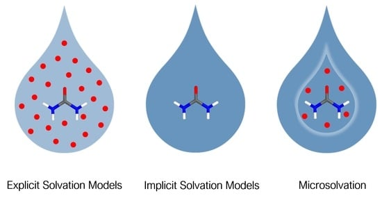
1. Introduction
2. Grid Inhomogeneous Solvation Theory (GIST)
3. Computational Methodology
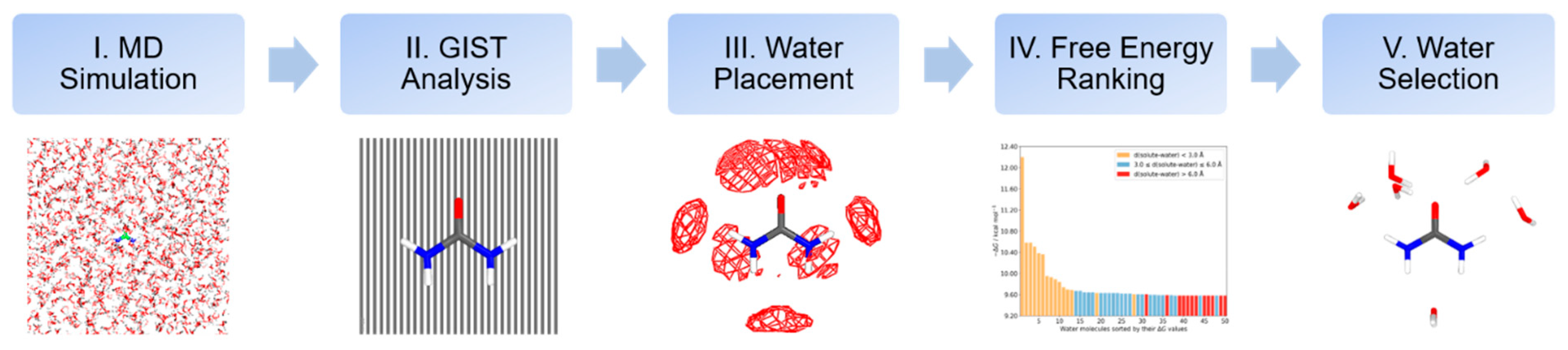
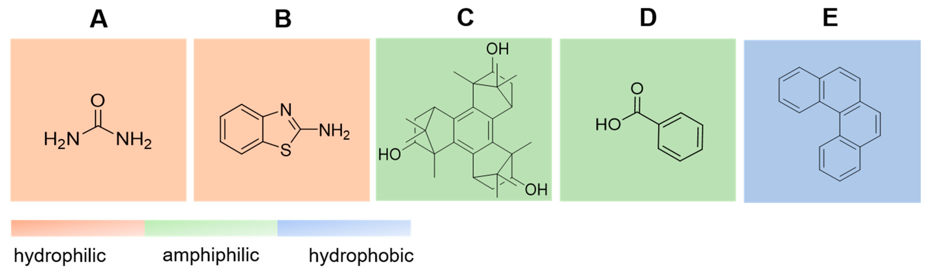
3.1. Computational Protocol to Microsolvation
3.2. Molecular Dynamics Simulation Details
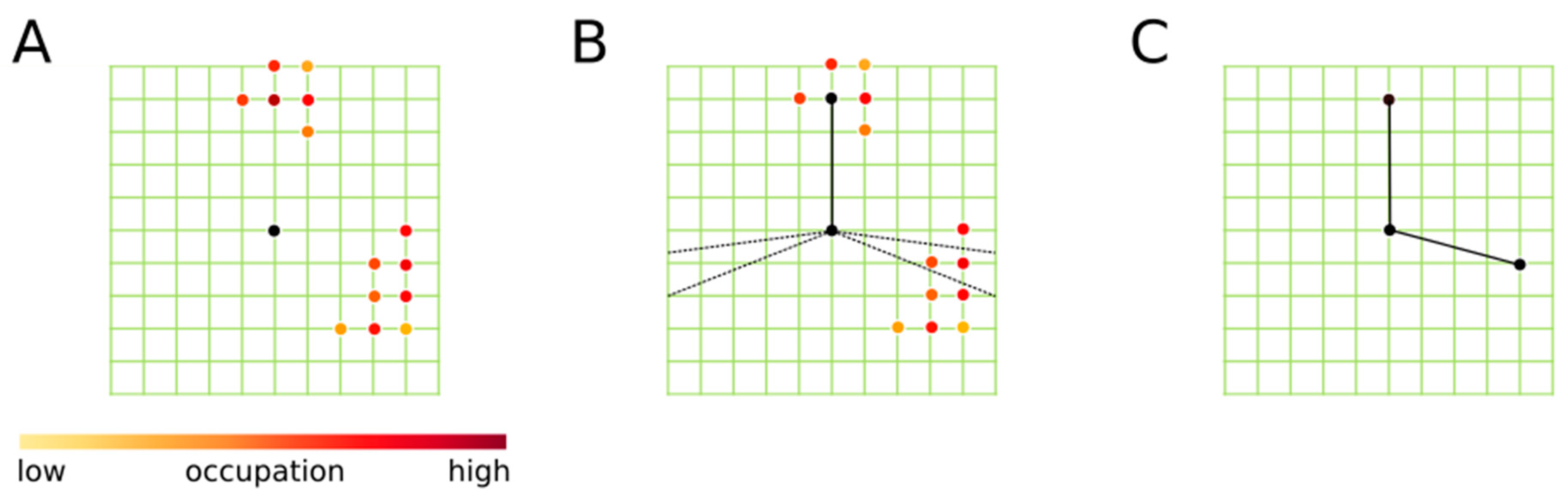
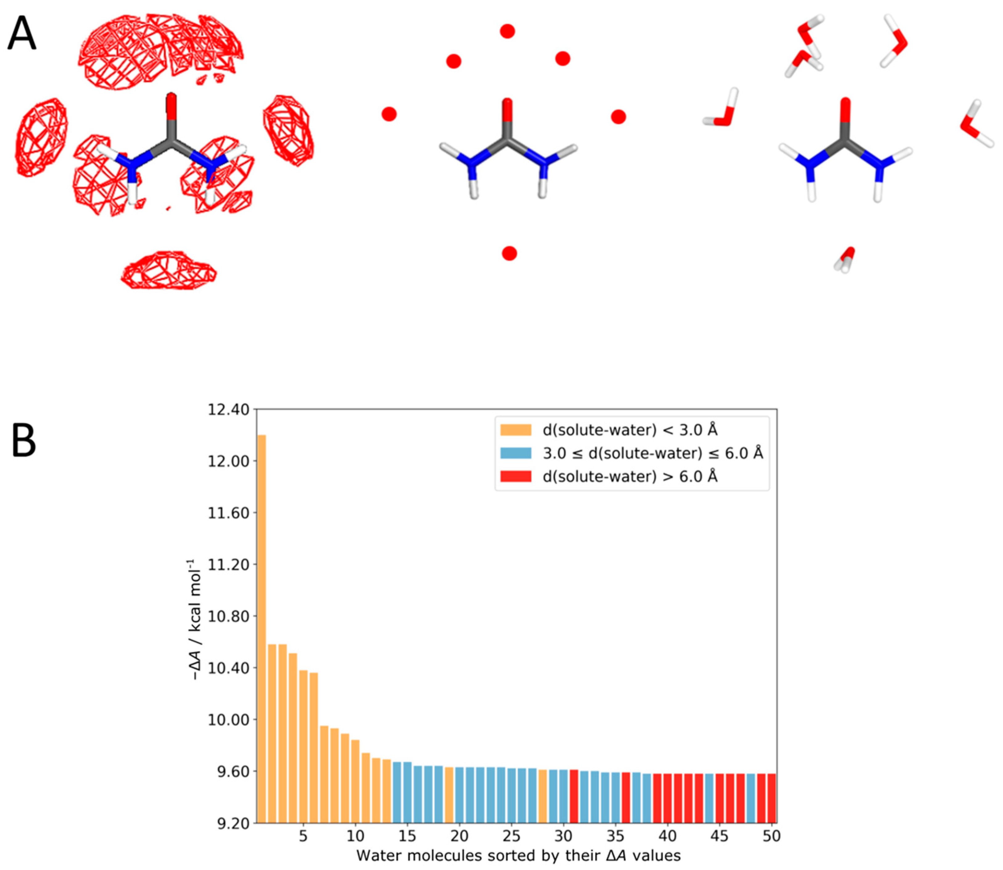
3.3. Data Analysis and Reference Settings
3.4. Quantum Chemical Calculations
4. Results
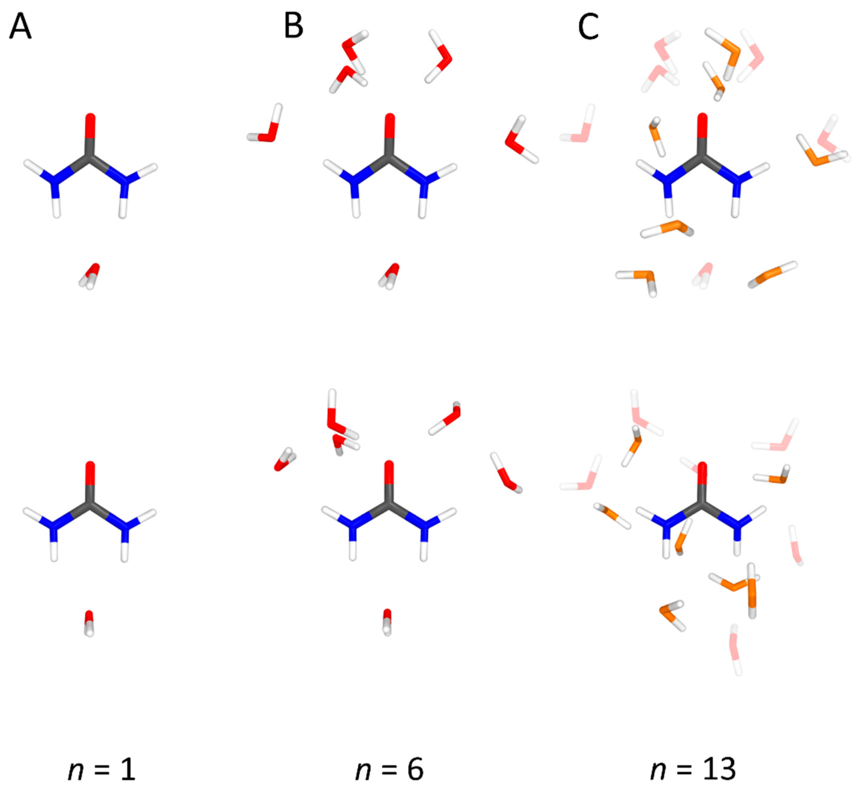
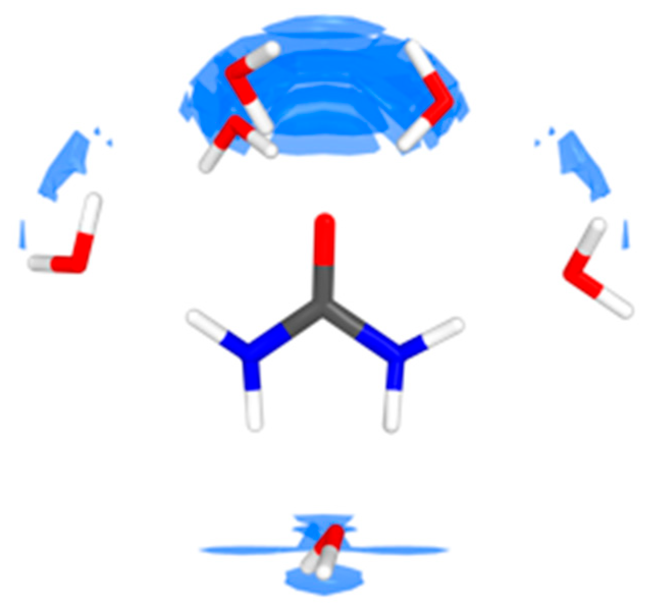
4.1. Urea–Water Complexes
4.2. Aminobenzothiazole–Water Complexes
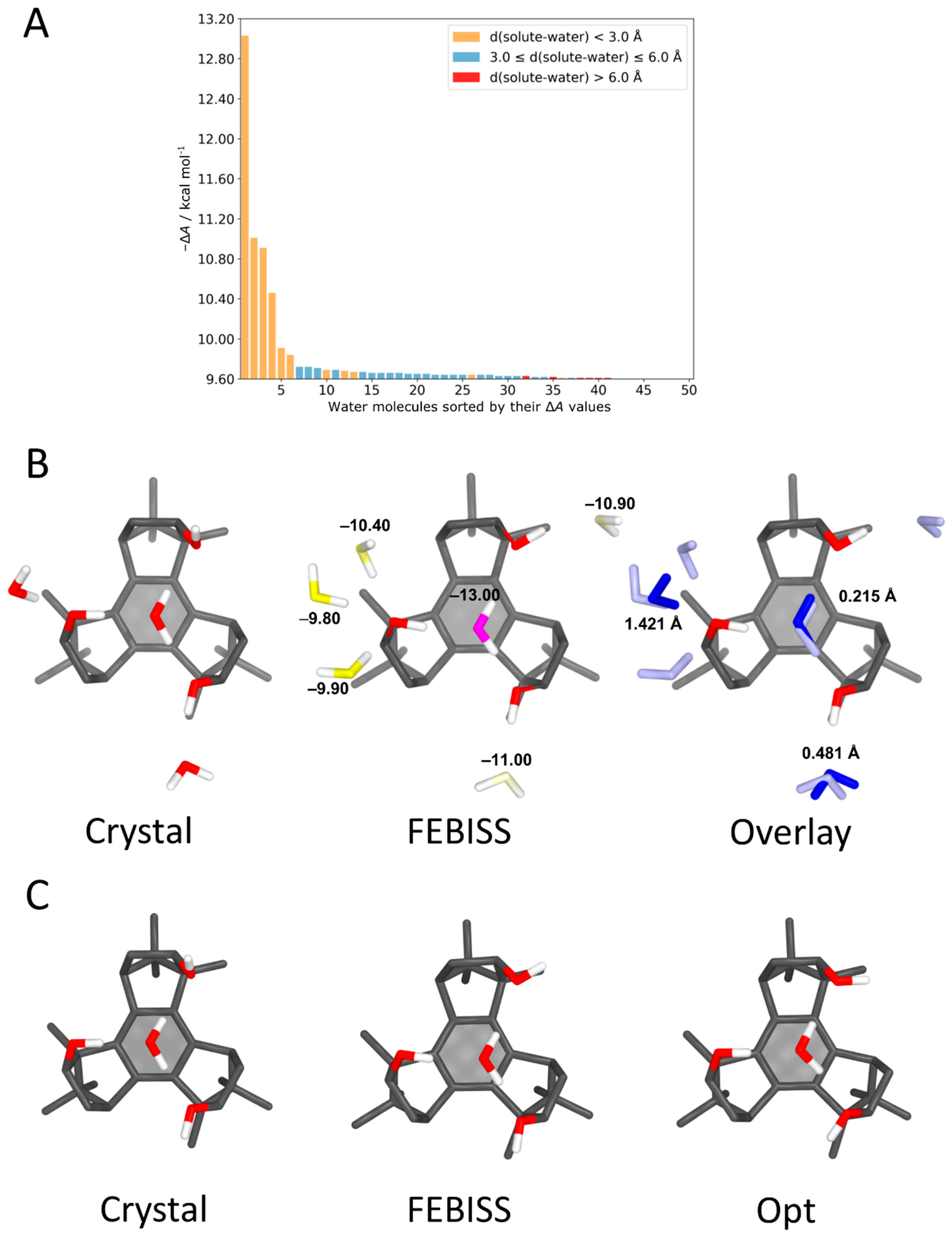
4.3. Benzotriborneol–Water Complexes
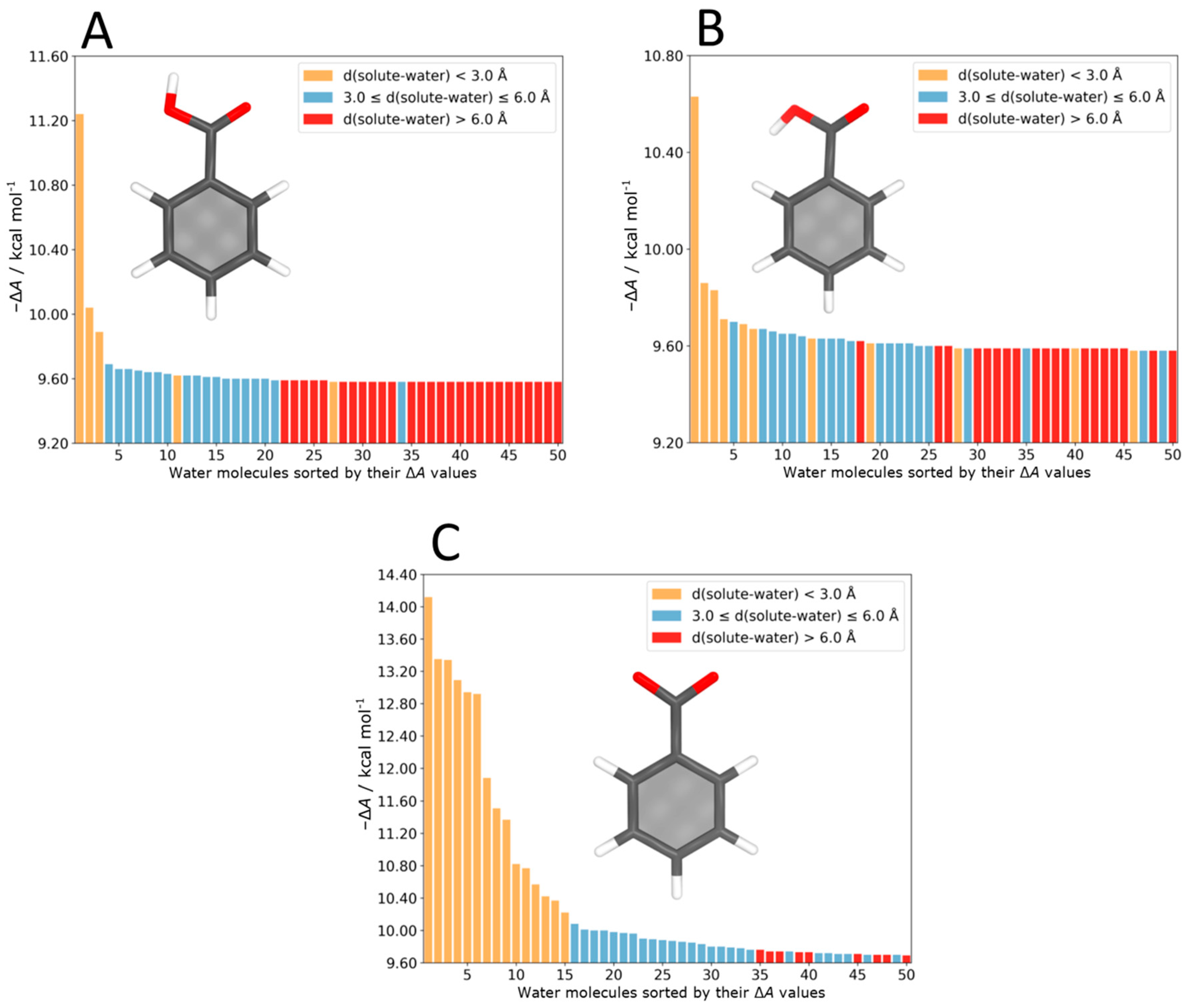
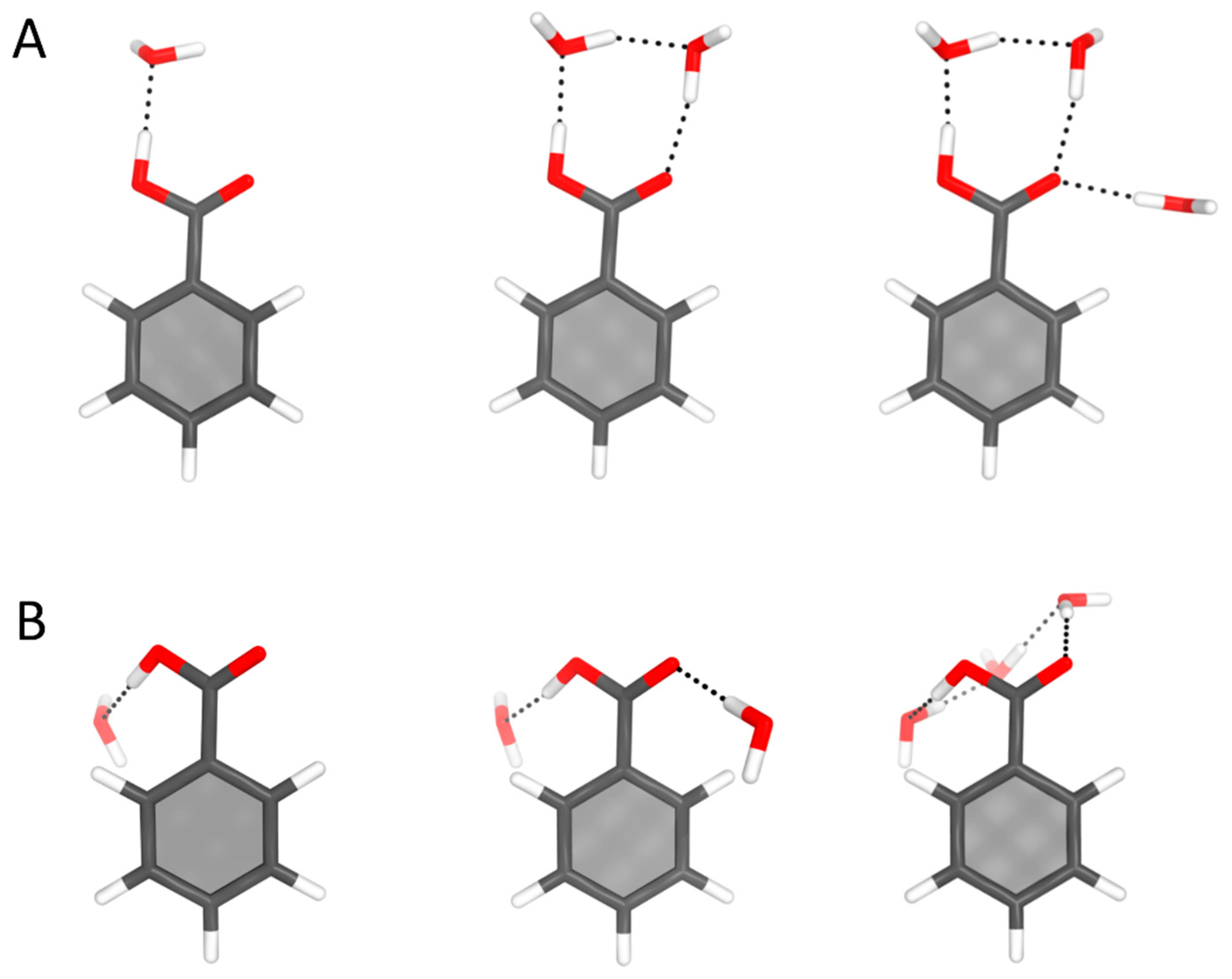
4.4. Benzoic Acid–Water Complexes
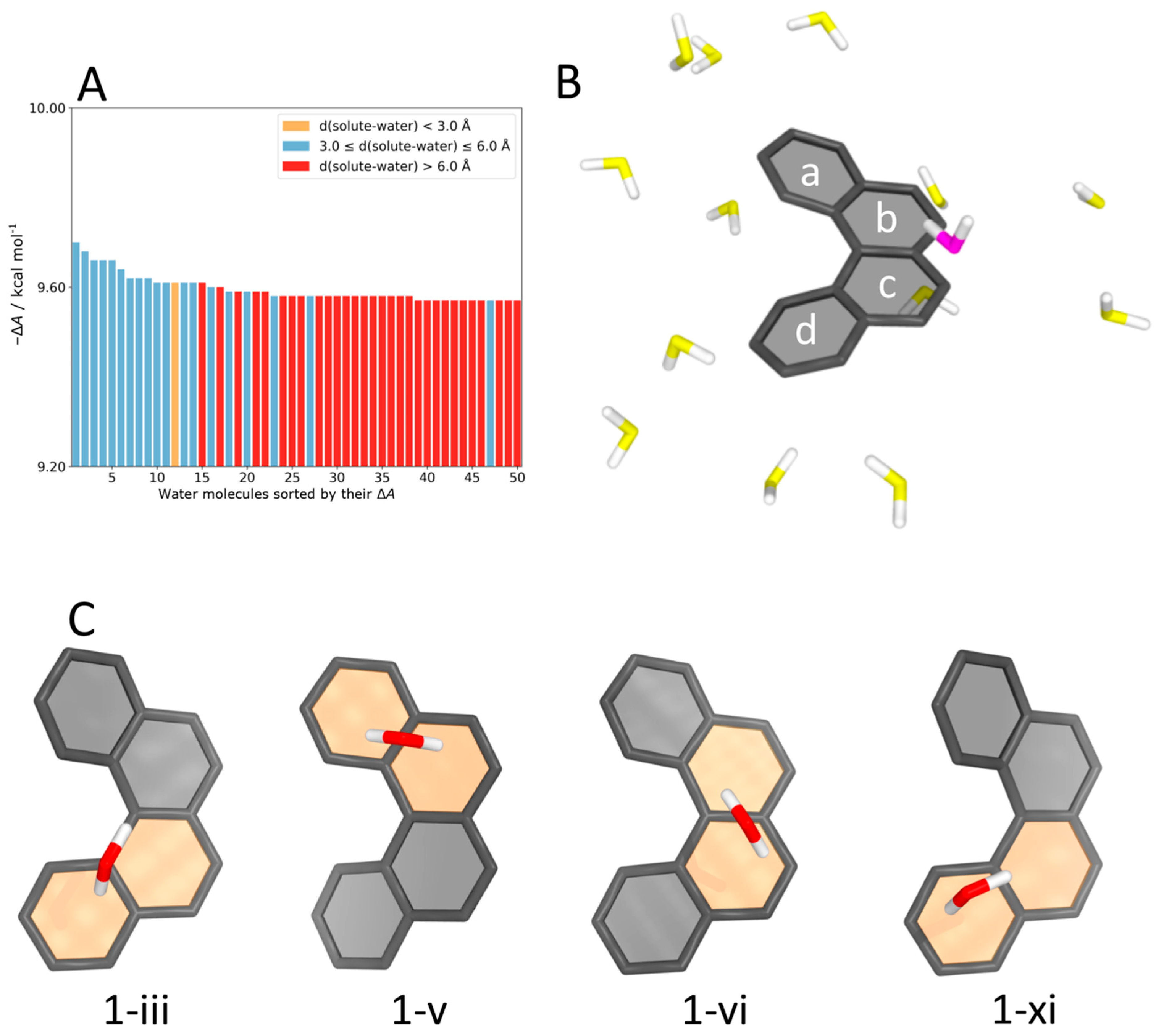
4.5. Helicene–Water Complexes
5. Discussion
6. Conclusions
Supplementary Materials
Author Contributions
Funding
Institutional Review Board Statement
Informed Consent Statement
Data Availability Statement
Acknowledgments
Conflicts of Interest
Sample Availability
References
- Sherwood, J.; Clark, J.H.; Fairlamb, I.J.S.; Slattery, J.M. Solvent effects in palladium catalysed cross-coupling reactions. Green Chem. 2019, 21, 2164–2213. [Google Scholar] [CrossRef]
- Pirrung, M.C. Acceleration of Organic Reactions through Aqueous Solvent Effects. Chem. Eur. J. 2006, 12, 1312–1317. [Google Scholar] [CrossRef] [PubMed]
- Reichardt, C. Solvents and Solvent Effects: An Introduction. Org. Process. Res. Dev. 2007, 11, 105–113. [Google Scholar] [CrossRef]
- Reichardt, C.; Welton, T. Solute-Solvent Interactions. In Solvents and Solvent Effects in Organic Chemistry; Wiley: Hoboken, NJ, USA, 2010; pp. 7–64. [Google Scholar]
- Elmi, A.; Cockroft, S.L. Quantifying Interactions and Solvent Effects Using Molecular Balances and Model Complexes. Acc. Chem. Res. 2021, 54, 92–103. [Google Scholar] [CrossRef]
- Varghese, J.J.; Mushrif, S.H. Origins of complex solvent effects on chemical reactivity and computational tools to investigate them: A review. React. Chem. Eng. 2019, 4, 165–206. [Google Scholar] [CrossRef]
- Sunoj, R.B.; Anand, M. Microsolvated transition state models for improved insight into chemical properties and reaction mechanisms. Phys. Chem. Chem. Phys. 2012, 14, 12715–12736. [Google Scholar] [CrossRef]
- Pliego, J.R.; Riveros, J.M. Hybrid discrete-continuum solvation methods. Wiley Interdiscip. Rev. Comput. Mol. Sci. 2020, 10, 25. [Google Scholar] [CrossRef]
- Cramer, C.J.; Truhlar, D.G. A Universal Approach to Solvation Modeling. Acc. Chem. Res. 2008, 41, 760–768. [Google Scholar] [CrossRef] [PubMed]
- Tomasi, J.; Mennucci, B.; Cammi, R. Quantum Mechanical Continuum Solvation Models. Chem. Rev. 2005, 105, 2999–3094. [Google Scholar] [CrossRef] [PubMed]
- Marenich, A.V.; Cramer, C.J.; Truhlar, D.G. Universal Solvation Model Based on Solute Electron Density and on a Continuum Model of the Solvent Defined by the Bulk Dielectric Constant and Atomic Surface Tensions. J. Phys. Chem. B 2009, 113, 6378–6396. [Google Scholar] [CrossRef] [PubMed]
- Klamt, A. The COSMO and COSMO-RS solvation models. Wiley Interdiscip. Rev. Comput. Mol. Sci. 2011, 1, 699–709. [Google Scholar] [CrossRef]
- Marx, D.; Hutter, J. Ab Initio Molecular Dynamics: Basic Theory and Advanced Methods; Cambridge University Press: Cambridge, UK, 2009. [Google Scholar]
- Hutter, J. Car-Parrinello molecular dynamics. Wiley Interdiscip. Rev. Comput. Mol. Sci. 2011, 2, 604–612. [Google Scholar] [CrossRef]
- Kühne, T.D. Second generation Car-Parrinello molecular dynamics. Wiley Interdiscip. Rev. Comput. Mol. Sci. 2014, 4, 391–406. [Google Scholar] [CrossRef]
- Kelly, C.P.; Cramer, C.J.; Truhlar, D.G. Adding Explicit Solvent Molecules to Continuum Solvent Calculations for the Calculation of Aqueous Acid Dissociation Constants. J. Phys. Chem. A 2006, 110, 2493–2499. [Google Scholar] [CrossRef] [PubMed]
- Thar, J.; Zahn, S.; Kirchner, B. When Is a Molecule Properly Solvated by a Continuum Model or in a Cluster Ansatz? A First-Principles Simulation of Alanine Hydration. J. Phys. Chem. B 2008, 112, 1456–1464. [Google Scholar] [CrossRef]
- Pliego, J.A.J.R.; Riveros, J.M. The Cluster−Continuum Model for the Calculation of the Solvation Free Energy of Ionic Species. J. Phys. Chem. A 2001, 105, 7241–7247. [Google Scholar] [CrossRef]
- Bryantsev, V.S.; Diallo, M.S.; Iii, W.A.G. Calculation of Solvation Free Energies of Charged Solutes Using Mixed Cluster/Continuum Models. J. Phys. Chem. B 2008, 112, 9709–9719. [Google Scholar] [CrossRef] [PubMed]
- Marenich, A.V.; Ding, W.; Cramer, C.J.; Truhlar, N.G. Resolution of a Challenge for Solvation Modeling: Calculation of Dicarboxylic Acid Dissociation Constants Using Mixed Discrete–Continuum Solvation Models. J. Phys. Chem. Lett. 2012, 3, 1437–1442. [Google Scholar] [CrossRef]
- Zins, E.-L. Microhydration of a Carbonyl Group: How does the Molecular Electrostatic Potential (MESP) Impact the Formation of (H2O)n:(R2C═O)Complexes? J. Phys. Chem. A 2020, 124, 1720–1734. [Google Scholar] [CrossRef]
- Gadre, S.R.; Babu, K.; Rendell, A.P. Electrostatics for Exploring Hydration Patterns of Molecules. 3. Uracil. J. Phys. Chem. A 2000, 104, 8976–8982. [Google Scholar] [CrossRef]
- Kalai, C.; Alikhani, M.E.; Zins, E.L. The molecular electrostatic potential analysis of solutes and water clusters: A straightforward tool to predict the geometry of the most stable micro-hydrated complexes of beta-propiolactone and formamide. Theor. Chem. Acc. 2018, 137, 20. [Google Scholar] [CrossRef]
- Sure, R.; El Mahdali, M.; Plajer, A.; Deglmann, P. Towards a converged strategy for including microsolvation in reaction mechanism calculations. J. Comput. Mol. Des. 2021, 20, 1–20. [Google Scholar] [CrossRef]
- Lanza, G.; Chiacchio, M.A. The water molecule arrangement over the side chain of some aliphatic amino acids: A quantum chemical and bottom-up investigation. Int. J. Quantum Chem. 2020, 120, 17. [Google Scholar] [CrossRef]
- Simm, G.N.; Türtscher, P.L.; Reiher, M. Systematic microsolvation approach with a cluster-continuum scheme and conformational sampling. J. Comput. Chem. 2020, 41, 1144–1155. [Google Scholar] [CrossRef] [PubMed]
- Basdogan, Y.; Groenenboom, M.C.; Henderson, E.; De, S.; Rempe, S.B.; Keith, J.A. Machine Learning-Guided Approach for Studying Solvation Environments. J. Chem. Theory Comput. 2019, 16, 633–642. [Google Scholar] [CrossRef] [PubMed]
- Jesus, W.S.; Prudente, F.V.; Marques, J.M.C.; Pereira, F.B. Modeling microsolvation clusters with electronic-structure calculations guided by analytical potentials and predictive machine learning techniques. Phys. Chem. Chem. Phys. 2021, 23, 1738–1749. [Google Scholar] [CrossRef]
- Kongsted, J.; Mennucci, B.; Coutinho, K.; Canuto, S. Solvent effects on the electronic absorption spectrum of camphor using continuum, discrete or explicit approaches. Chem. Phys. Lett. 2010, 484, 185–191. [Google Scholar] [CrossRef]
- Mensch, C.; Bultinck, P.; Johannessen, C. The effect of protein backbone hydration on the amide vibrations in Raman and Raman optical activity spectra. Phys. Chem. Chem. Phys. 2019, 21, 1988–2005. [Google Scholar] [CrossRef] [PubMed]
- Da Silva, E.F.; Svendsen, H.F.; Merz, K.M. Explicitly Representing the Solvation Shell in Continuum Solvent Calculations. J. Phys. Chem. A 2009, 113, 6404–6409. [Google Scholar] [CrossRef]
- Nocito, D.; Beran, G.J.O. Averaged Condensed Phase Model for Simulating Molecules in Complex Environments. J. Chem. Theory Comput. 2017, 13, 1117–1129. [Google Scholar] [CrossRef]
- Karimova, N.V.; Luo, M.; Grassian, V.H.; Gerber, R.B. Absorption spectra of benzoic acid in water at different pH and in the presence of salts: Insights from the integration of experimental data and theoretical cluster models. Phys. Chem. Chem. Phys. 2020, 22, 5046–5056. [Google Scholar] [CrossRef]
- Basdogan, Y.; Maldonado, A.M.; Keith, J.A. Advances and challenges in modeling solvated reaction mechanisms for renewable fuels and chemicals. Wiley Interdiscip. Rev. Comput. Mol. Sci. 2020, 10, 19. [Google Scholar] [CrossRef]
- Bodnarchuk, M.S.; Viner, R.; Michel, J.; Essex, J.W. Strategies to Calculate Water Binding Free Energies in Protein–Ligand Complexes. J. Chem. Inf. Model. 2014, 54, 1623–1633. [Google Scholar] [CrossRef] [PubMed]
- Spyrakis, F.; Ahmed, M.H.; Bayden, A.S.; Cozzini, P.; Mozzarelli, A.; Kellogg, G.E. The Roles of Water in the Protein Matrix: A Largely Untapped Resource for Drug Discovery. J. Med. Chem. 2017, 60, 6781–6827. [Google Scholar] [CrossRef]
- Bucher, D.; Stouten, P.F.; Triballeau, N. Shedding Light on Important Waters for Drug Design: Simulations versus Grid-Based Methods. J. Chem. Inf. Model. 2018, 58, 692–699. [Google Scholar] [CrossRef]
- Rudling, A.; Orro, A.; Carlsson, J. Prediction of Ordered Water Molecules in Protein Binding Sites from Molecular Dynamics Simulations: The Impact of Ligand Binding on Hydration Networks. J. Chem. Inf. Model. 2018, 58, 350–361. [Google Scholar] [CrossRef] [PubMed]
- Jukic, M.; Konc, J.; Janezic, D.; Bren, U. ProBiS H2O MD Approach for Identification of Conserved Water Sites in Protein Structures for Drug Design. ACS Med. Chem. Lett. 2020, 11, 877–882. [Google Scholar] [CrossRef]
- Kearney, B.M.; Schwabe, M.; Marcus, K.C.; Roberts, D.M.; DeChene, M.; Swartz, P.; Mattos, C. DRoP: Automated detection of conserved solvent-binding sites on proteins. Proteins Struct. Funct. Bioinform. 2020, 88, 152–165. [Google Scholar] [CrossRef]
- Ramsey, S.; Nguyen, C.; Salomon-Ferrer, R.; Walker, R.C.; Gilson, M.K.; Kurtzman, T. Solvation thermodynamic mapping of molecular surfaces in AmberTools: GIST. J. Comput. Chem. 2016, 37, 2029–2037. [Google Scholar] [CrossRef]
- Nguyen, C.N.; Young, T.K.; Gilson, M.K. Grid inhomogeneous solvation theory: Hydration structure and thermodynamics of the miniature receptor cucurbit[7]uril. J. Chem. Phys. 2012, 137, 044101. [Google Scholar] [CrossRef]
- Nguyen, C.N.; Cruz, A.; Gilson, M.K.; Kurtzman, T. Thermodynamics of Water in an Enzyme Active Site: Grid-Based Hydration Analysis of Coagulation Factor Xa. J. Chem. Theory Comput. 2014, 10, 2769–2780. [Google Scholar] [CrossRef]
- Loeffler, J.R.; Schauperl, M.; Liedl, K.R. Hydration of Aromatic Heterocycles as an Adversary of pi-Stacking. J. Chem. Inf. Model. 2019, 59, 4209–4219. [Google Scholar] [CrossRef]
- Loeffler, J.R.; Fernández-Quintero, M.L.; Schauperl, M.; Liedl, K.R. STACKED – Solvation Theory of Aromatic Complexes as Key for Estimating Drug Binding. J. Chem. Inf. Model. 2020, 60, 2304–2313. [Google Scholar] [CrossRef]
- Schauperl, M.; Czodrowski, P.; Fuchs, J.E.; Huber, R.G.; Waldner, B.J.; Podewitz, M.; Kramer, C.; Liedl, K.R. Binding Pose Flip Explained via Enthalpic and Entropic Contributions. J. Chem. Inf. Model. 2017, 57, 345–354. [Google Scholar] [CrossRef] [PubMed]
- Schauperl, M.; Podewitz, M.; Ortner, T.S.; Waibl, F.; Thoeny, A.; Loerting, T.; Liedl, K.R. Balance between hydration enthalpy and entropy is important for ice binding surfaces in Antifreeze Proteins. Sci. Rep. 2017, 7, 11901. [Google Scholar] [CrossRef]
- Fabris, F.; De Lucchi, O.; Nardini, I.; Crisma, M.; Mazzanti, A.; Mason, S.A.; Lemée-Cailleau, M.-H.; Scaramuzzo, F.A.; Zonta, C. (+)-syn-Benzotriborneol an enantiopure C3-symmetric receptor for water. Org. Biomol. Chem. 2012, 10, 2464–2469. [Google Scholar] [CrossRef]
- Wazzan, N.; Safi, Z.; Al-Barakati, R.; Al-Qurashi, O.; Al-Khateeb, L. DFT investigation on the intramolecular and intermolecular proton transfer processes in 2-aminobenzothiazole (ABT) in the gas phase and in different solvents. Struct. Chem. 2019, 31, 243–252. [Google Scholar] [CrossRef]
- Ishida, T.; Rossky, P.J.; Castner, E.W. A Theoretical Investigation of the Shape and Hydration Properties of Aqueous Urea: Evidence for Nonplanar Urea Geometry. J. Phys. Chem. B 2004, 108, 17583–17590. [Google Scholar] [CrossRef]
- Domingos, S.R.; Martin, K.; Avarvari, N.; Schnell, M. Water Docking Bias in 4 Helicene. Angew. Chem. Int. Ed. 2019, 58, 11257–11261. [Google Scholar] [CrossRef] [PubMed]
- Weiss, A.K.H.; Hofer, T.S. Urea in aqueous solution studied by quantum mechanical charge field-molecular dynamics (QMCF-MD). Mol. BioSyst. 2013, 9, 1864–1876. [Google Scholar] [CrossRef] [PubMed]
- Bruno, G.; Randaccio, L. A refinement of the benzoic acid structure at room temperature. Acta Crystallogr. Sect. B Struct. Crystallogr. Cryst. Chem. 1980, 36, 1711–1712. [Google Scholar] [CrossRef]
- Nagy, P.I.; Smith, D.A.; Alagona, G.; Ghio, C. Ab initio studies of free and monohydrated carboxylic acids in the gas phase. J. Phys. Chem. 1994, 98, 486–493. [Google Scholar] [CrossRef]
- Stepanian, S.; Reva, I.; Radchenko, E.; Sheina, G. Infrared spectra of benzoic acid monomers and dimers in argon matrix. Vib. Spectrosc. 1996, 11, 123–133. [Google Scholar] [CrossRef]
- Godfrey, P.D.; McNaughton, D. Structural studies of aromatic carboxylic acids via computational chemistry and microwave spectroscopy. J. Chem. Phys. 2013, 138, 24303. [Google Scholar] [CrossRef] [PubMed]
- Schnitzler, E.G.; Jäger, W. The benzoic acid–water complex: A potential atmospheric nucleation precursor studied using microwave spectroscopy and ab initio calculations. Phys. Chem. Chem. Phys. 2014, 16, 2305–2314. [Google Scholar] [CrossRef] [PubMed]
- Onda, M.; Asai, M.; Takise, K.; Kuwae, K.; Hayami, K.; Kuroe, A.; Mori, M.; Miyazaki, H.; Suzuki, N.; Yamaguchi, I. Microwave spectrum of benzoic acid. J. Mol. Struct. 1999, 482-483, 301–303. [Google Scholar] [CrossRef]
- Aarset, K.; Page, E.M.; Rice, D.A. Molecular Structures of Benzoic Acid and 2-Hydroxybenzoic Acid, Obtained by Gas-Phase Electron Diffraction and Theoretical Calculations. J. Phys. Chem. A 2006, 110, 9014–9019. [Google Scholar] [CrossRef]
- Lazaridis, T. Inhomogeneous Fluid Approach to Solvation Thermodynamics. 1. Theory. J. Phys. Chem. B 1998, 102, 3531–3541. [Google Scholar] [CrossRef]
- Roe, D.R.; Cheatham, T.E. PTRAJ and CPPTRAJ: Software for Processing and Analysis of Molecular Dynamics Trajectory Data. J. Chem. Theory Comput. 2013, 9, 3084–3095. [Google Scholar] [CrossRef]
- Jorgensen, W.L.; Chandrasekhar, J.; Madura, J.D.; Impey, R.W.; Klein, M.L. Comparison of simple potential functions for simulating liquid water. J. Chem. Phys. 1983, 79, 926–935. [Google Scholar] [CrossRef]
- Salomon-Ferrer, R.; Case, D.A.; Walker, R.C. An overview of the Amber biomolecular simulation package. Wiley Interdiscip. Rev. Comput. Mol. Sci. 2013, 3, 198–210. [Google Scholar] [CrossRef]
- Case, D.A.; Ben-Shalom, I.Y.; Brozell, S.R.; Cerutti, D.S.; Cheatham, I.T.E.; Cruzeiro, V.W.D.; Darden, T.A.; Duke, R.E.; Ghoreishi, D.; Gilson, M.K.; et al. AMBER 2018; University of California: San Francisco, CA, USA, 2018. [Google Scholar]
- The PyMOL Molecular Graphics System, Version 1.8. Available online: https://sourceforge.net/projects/pymol/files/pymol/1.8/ (accessed on 25 February 2021).
- Available online: https://github.com/PodewitzLab/FEBISS.git (accessed on 25 February 2021).
- Available online: https://github.com/liedllab/gigist (accessed on 25 February 2021).
- Kraml, J.; Kamenik, A.S.; Waibl, F.; Schauperl, M.; Liedl, K.R. Solvation Free Energy as a Measure of Hydrophobicity: Application to Serine Protease Binding Interfaces. J. Chem. Theory Comput. 2019, 15, 5872–5882. [Google Scholar] [CrossRef] [PubMed]
- Frisch, M.J.; Trucks, G.W.; Schlegel, H.B.; Scuseria, G.E.; Robb, M.A.; Cheeseman, J.R.; Scalmani, G.; Barone, V.; Petersson, G.A.; Nakatsuji, H.; et al. Gaussian 16 Rev. C.01; Gaussian, Inc.: Wallingford, CT, USA, 2016. [Google Scholar]
- Bayly, C.I.; Cieplak, P.; Cornell, W.; Kollman, P.A. A well-behaved electrostatic potential based method using charge restraints for deriving atomic charges: The RESP model. J. Phys. Chem. 1993, 97, 10269–10280. [Google Scholar] [CrossRef]
- Jakalian, A.; Jack, D.B.; Bayly, C.I. Fast, efficient generation of high-quality atomic charges. AM1-BCC model: II. Parameterization and validation. J. Comput. Chem. 2002, 23, 1623–1641. [Google Scholar] [CrossRef]
- Wang, J.; Wolf, R.M.; Caldwell, J.W.; Kollman, P.A.; Case, D.A. Development and testing of a general amber force field. J. Comput. Chem. 2004, 25, 1157–1174. [Google Scholar] [CrossRef]
- Wallnoefer, H.G.; Liedl, K.R.; Fox, T. A challenging system: Free energy prediction for factor Xa. J. Comput. Chem. 2011, 32, 1743–1752. [Google Scholar] [CrossRef] [PubMed]
- Salomon-Ferrer, R.; Götz, A.W.; Poole, D.; Le Grand, S.; Walker, R.C. Routine Microsecond Molecular Dynamics Simulations with AMBER on GPUs. 2. Explicit Solvent Particle Mesh Ewald. J. Chem. Theory Comput. 2013, 9, 3878–3888. [Google Scholar] [CrossRef] [PubMed]
- Adelman, S.A.; Doll, J.D. Generalized Langevin Equation Approach for Atom-Solid-Surface Scattering: General Formulation for Classical Scattering off Harmonic Solids. J. Chem. Phys. 1976, 64, 2375–2388. [Google Scholar] [CrossRef]
- Darden, T.; York, D.; Pedersen, L. Particle mesh Ewald: An N·log(N) method for Ewald sums in large systems. J. Chem. Phys. 1993, 98, 10089–10092. [Google Scholar] [CrossRef]
- Ryckaert, J.-P.; Ciccotti, G.; Berendsen, H.J.C. Numerical integration of the cartesian equations of motion of a system with constraints: Molecular dynamics of n-alkanes. J. Comput. Phys. 1977, 23, 327–341. [Google Scholar] [CrossRef]
- Kovalenko, A.; Hirata, F. Self-consistent description of a metal–water interface by the Kohn–Sham density functional theory and the three-dimensional reference interaction site model. J. Chem. Phys. 1999, 110, 10095–10112. [Google Scholar] [CrossRef]
- Group, C.C. Molecular Operating Environment; 2018. [Google Scholar]
- Furche, F.; Ahlrichs, R.; Hättig, C.; Klopper, W.; Sierka, M.; Weigend, F. Turbomole. Wiley Interdiscip. Rev. Comput. Mol. 2014, 4, 91–100. [Google Scholar] [CrossRef]
- TURBOMOLE V7.3 2018, a Development of University of Karlsruhe and Forschungszentrum Karlsruhe GmbH, 1989–2007, TURBOMOLE GmbH, Since 2007. Available online: http://www.turbomole.com/ (accessed on 25 February 2021).
- Becke, A.D. Density-Functional Thermochemistry III. The Role of Exact Exchange. J. Chem. Phys. 1993, 98, 5648–5652. [Google Scholar] [CrossRef]
- Lee, C.; Yang, W.; Parr, R.G. Development of the Colle-Salvetti correlation-energy formula into a functional of the electron density. Phys. Rev. B 1988, 37, 785–789. [Google Scholar] [CrossRef] [PubMed]
- Becke, A.D. Density-functional exchange-energy approximation with correct asymptotic behavior. Phys. Rev. A 1988, 38, 3098–3100. [Google Scholar] [CrossRef] [PubMed]
- Weigend, F.; Ahlrichs, R. Balanced Basis Sets of Split Valence, Triple Zeta Valence and Quadruple Zeta Valence Quality For H to Rn: Design and Assessment of Accuracy. Phys. Chem. Chem. Phys. 2005, 7, 3297–3305. [Google Scholar] [CrossRef] [PubMed]
- Grimme, S.; Antony, J.; Ehrlich, S.; Krieg, H. A consistent and accurate ab initio parametrization of density functional dispersion correction (DFT-D) for the 94 elements H-Pu. J. Chem. Phys. 2010, 132, 154104. [Google Scholar] [CrossRef]
- Grimme, S.; Ehrlich, S.; Goerigk, L. Effect of the damping function in dispersion corrected density functional theory. J. Comput. Chem. 2011, 32, 1456–1465. [Google Scholar] [CrossRef] [PubMed]
- Klamt, A.; Schüürmann, G. COSMO: A new approach to dielectric screening in solvents with explicit expressions for the screening energy and its gradient. J. Chem. Soc. Perkin Trans. 2 1993, 5, 799–805. [Google Scholar] [CrossRef]
- Schäfer, A.; Klamt, A.; Sattel, D.; Lohrenz, J.C.W.; Eckert, F. COSMO Implementation in TURBOMOLE: Extension of an efficient quantum chemical code towards liquid systems. Phys. Chem. Chem. Phys. 2000, 2, 2187–2193. [Google Scholar] [CrossRef]
- Hirschfeld, F.L.; Schmidt, G.M.J.; Sandler, S. 398.The Structure of Overcrowded Aromatic Compounds. Part VI. The Crystal Structure of Benzo[C]phenanthrene and of 1,12-Dimethylbenzo[C]phenanthrene. J. Chem. Soc. 1963, 2108–2125. [Google Scholar] [CrossRef]
- Mobley, D.L.; Dumont, É.; Chodera, J.D.; Dill, K.A. Comparison of Charge Models for Fixed-Charge Force Fields: Small-Molecule Hydration Free Energies in Explicit Solvent. J. Phys. Chem. B 2007, 111, 2242–2254. [Google Scholar] [CrossRef]
- Mobley, D.L.; Bayly, C.I.; Cooper, M.D.; Shirts, M.R.; Dill, K.A. Small Molecule Hydration Free Energies in Explicit Solvent: An Extensive Test of Fixed-Charge Atomistic Simulations. J. Chem. Theory Comput. 2009, 5, 350–358. [Google Scholar] [CrossRef]
- Shivakumar, D.; Deng, Y.; Roux, B. Computations of Absolute Solvation Free Energies of Small Molecules Using Explicit and Implicit Solvent Model. J. Chem. Theory Comput. 2009, 5, 919–930. [Google Scholar] [CrossRef]
- Bunken, C.; Reiher, M. Self-Parametrizing System-Focused Atomistic Models. J. Chem. Theory Comput. 2020, 16, 1646–1665. [Google Scholar] [CrossRef] [PubMed]
- Agieienko, V.; Buchner, R. Urea hydration from dielectric relaxation spectroscopy: Old findings confirmed, new insights gained. Phys. Chem. Chem. Phys. 2015, 18, 2597–2607. [Google Scholar] [CrossRef] [PubMed]
- Åstrand, P.-O.; Wallqvist, A.; Karlström, G.; Linse, P. Properties of Urea–Water Solvation Calculated from a New ab initio Polarizable Intermolecular Potential. J. Chem. Phys. 1991, 95, 8419–8429. [Google Scholar] [CrossRef]
- Kallies, B. Coupling of solvent and solute dynamics—Molecular dynamics simulations of aqueous urea solutions with different intramolecular potentials. Phys. Chem. Chem. Phys. 2001, 4, 86–95. [Google Scholar] [CrossRef]
- Stumpe, M.C.; Grubmüller, H. Aqueous Urea Solutions: Structure, Energetics, and Urea Aggregation. J. Phys. Chem. B 2007, 111, 6220–6228. [Google Scholar] [CrossRef] [PubMed]
- Krishnakumar, P.; Maity, D.K. Microhydration of a benzoic acid molecule and its dissociation. New J. Chem. 2017, 41, 7195–7202. [Google Scholar] [CrossRef]
- Chen, J.; Chan, B.; Shao, Y.; Ho, J. How accurate are approximate quantum chemical methods at modelling solute–solvent interactions in solvated clusters? Phys. Chem. Chem. Phys. 2020, 22, 3855–3866. [Google Scholar] [CrossRef] [PubMed]


| Structure | BA | BA-(H2O) | BA-(H2O)2 | BA-(H2O)3 |
|---|---|---|---|---|
| ΔEgas(syn-anti) | −6.0 | −9.0 | −13.4 | −2.3 |
| ΔEsolv(syn-anti) | −3.2 | −2.7 | −6.2 | −2.2 |
Publisher’s Note: MDPI stays neutral with regard to jurisdictional claims in published maps and institutional affiliations. |
© 2021 by the authors. Licensee MDPI, Basel, Switzerland. This article is an open access article distributed under the terms and conditions of the Creative Commons Attribution (CC BY) license (http://creativecommons.org/licenses/by/4.0/).
Share and Cite
Steiner, M.; Holzknecht, T.; Schauperl, M.; Podewitz, M. Quantum Chemical Microsolvation by Automated Water Placement. Molecules 2021, 26, 1793. https://doi.org/10.3390/molecules26061793
Steiner M, Holzknecht T, Schauperl M, Podewitz M. Quantum Chemical Microsolvation by Automated Water Placement. Molecules. 2021; 26(6):1793. https://doi.org/10.3390/molecules26061793
Chicago/Turabian StyleSteiner, Miguel, Tanja Holzknecht, Michael Schauperl, and Maren Podewitz. 2021. "Quantum Chemical Microsolvation by Automated Water Placement" Molecules 26, no. 6: 1793. https://doi.org/10.3390/molecules26061793
APA StyleSteiner, M., Holzknecht, T., Schauperl, M., & Podewitz, M. (2021). Quantum Chemical Microsolvation by Automated Water Placement. Molecules, 26(6), 1793. https://doi.org/10.3390/molecules26061793