
Calculation Methods of Solution Chemical Potential and Application in Emulsion Microencapsulation


Abstract
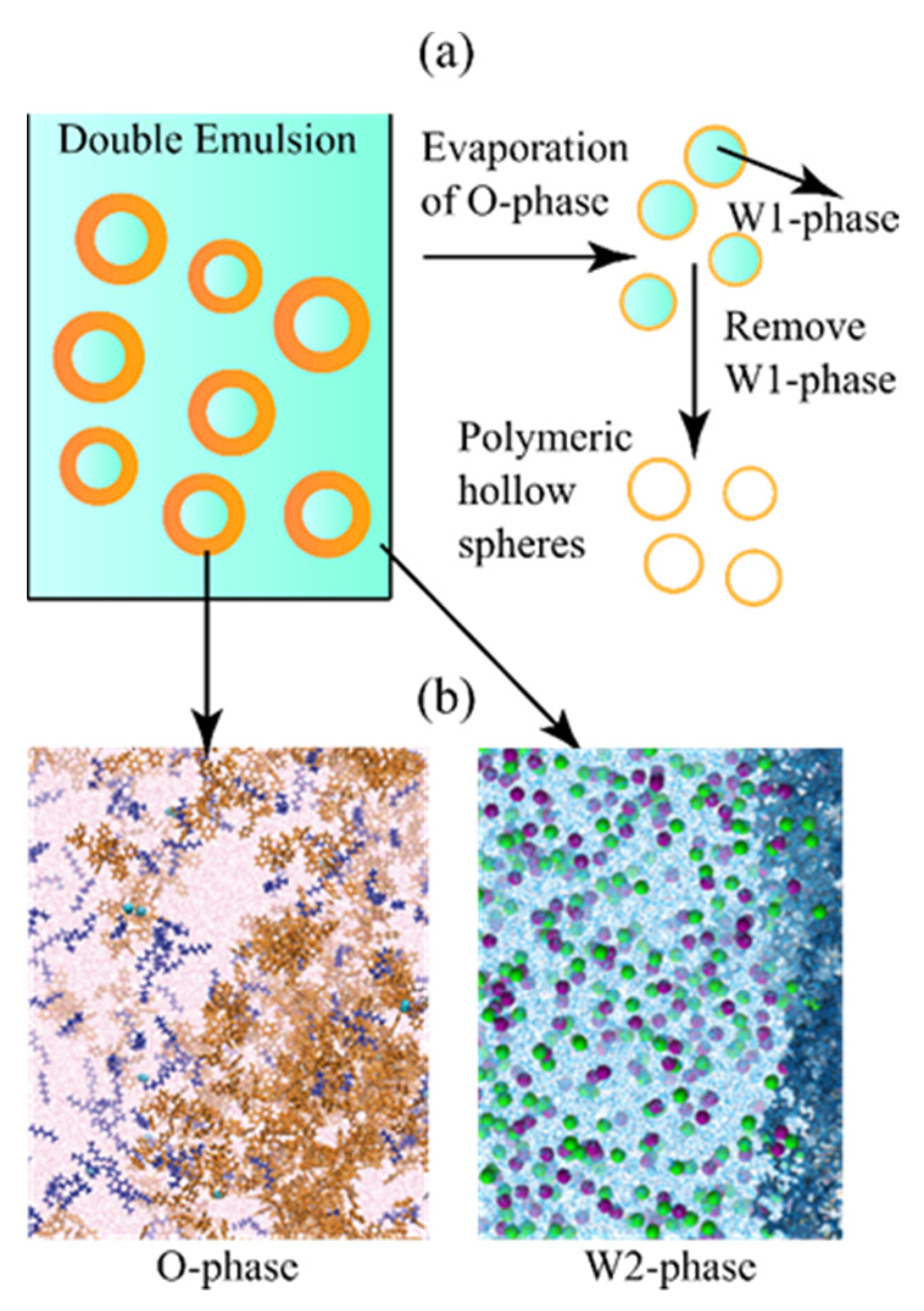
1. Introduction
2. Widom Insertion Method
2.1. Principle
2.2. Application of the Conventional Widom Method
3. Optimization of Widom Method Based on Biased Sampling
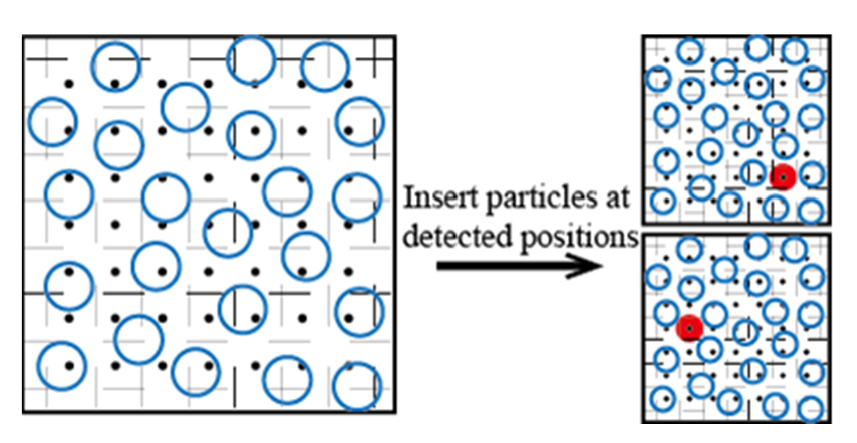
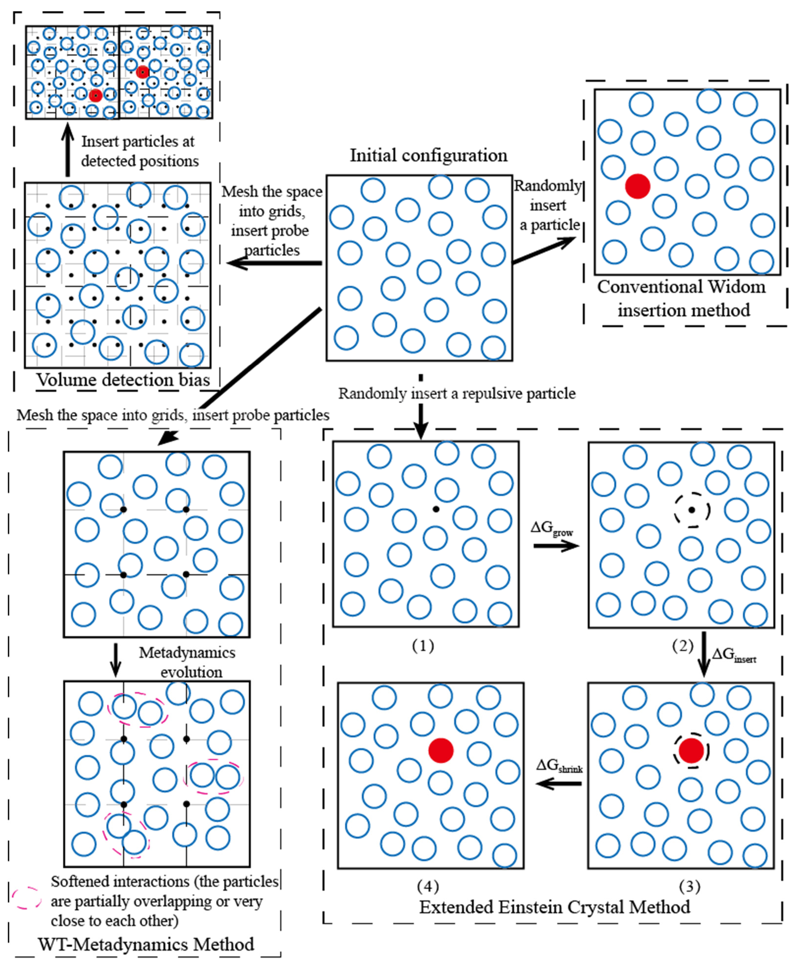
3.1. Volume Detection Bias
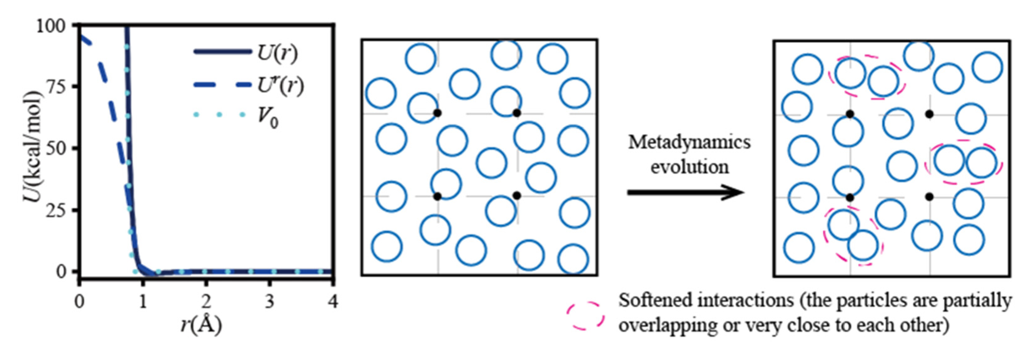
3.2. Simulation Ensemble Bias
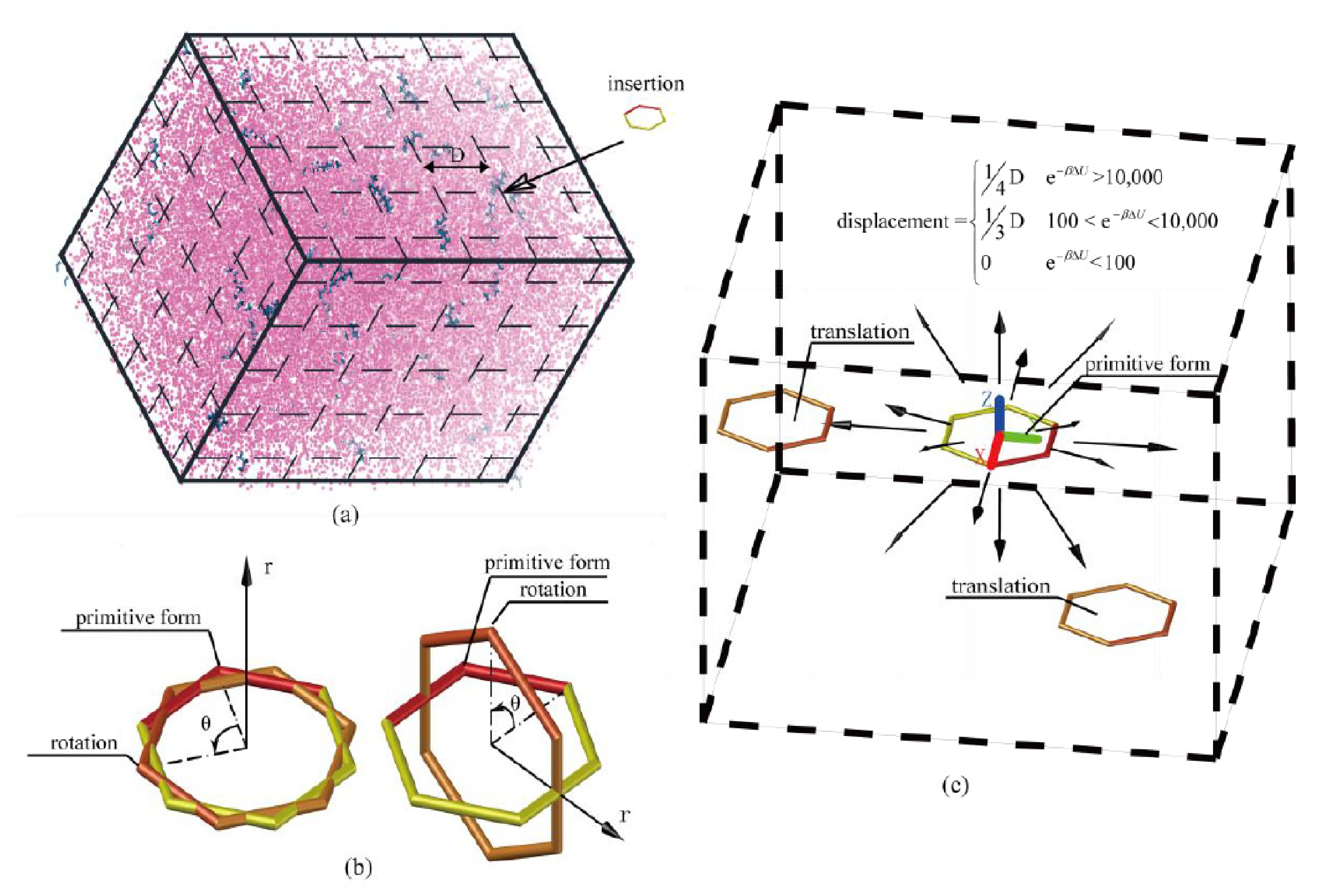
3.3. Particle Insertion Bias
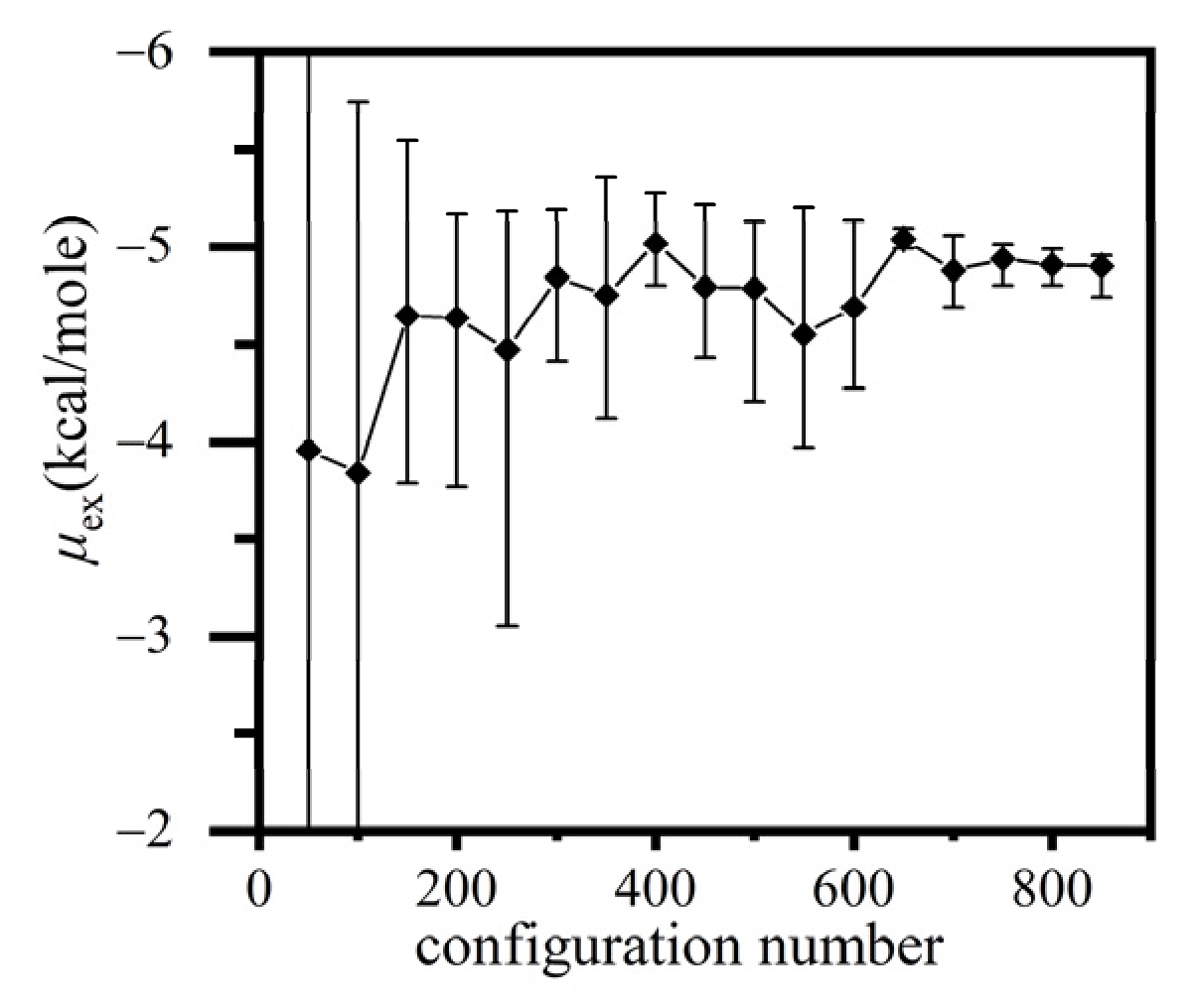
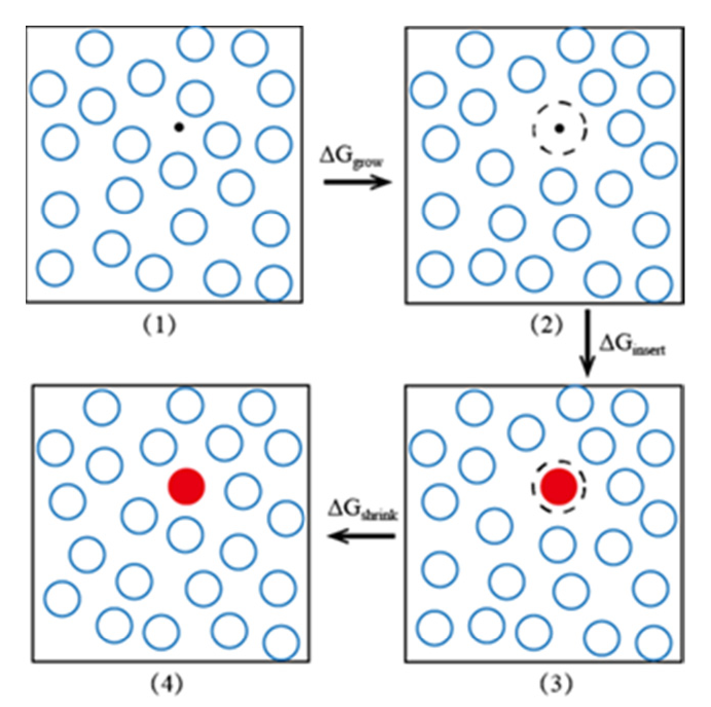
3.3.1. Extended Einstein Crystal Method (EECM)
3.3.2. Rosenbluth Sampling
3.4. Analysis on the Applicability of Various Biased Widom Insertion Methods for Emulsion Microencapsulation Solutions
4. Conclusions
Author Contributions
Funding
Institutional Review Board Statement
Informed Consent Statement
Data Availability Statement
Acknowledgments
Conflicts of Interest
References
- Cheng, C.J.; Chu, L.Y.; Ren, P.W.; Zhang, J.; Hu, L. Preparation of monodisperse thermo-sensitive poly(N-isopropylacrylamide) hollow microcapsules. J. Colloid Interface Sci. 2007, 313, 383–388. [Google Scholar] [CrossRef] [PubMed]
- Borodina, T.; Markvicheva, E.; Kunizhev, S.; Moehwald, H.; Sukhorukov, G.; Kreft, O. Controlled release of DNA from self-degrading microcapsules. Macromol. Rapid Commun. 2007, 28, 1894–1899. [Google Scholar] [CrossRef]
- Rabiei, A.; O’Neill, A. A study on processing of a composite metal foam via casting. Mater. Sci. Eng. A 2005, 404, 159–164. [Google Scholar] [CrossRef]
- Chang, C.J.; Jones, C.E.; Weinstein, B. Method for Preparing Ultraviolet Radiation-Absorbing Compositions. U.S. Patent 6,384,104 B1, 7 May 2002. [Google Scholar]
- Fang, Y.; Kuang, S.; Zhang, Z.; Gao, X. Preparation of nano-encapsulated phase change materials. J. Chem. Ind. 2007, 58, 771–775. [Google Scholar]
- Zhang, C.; Dai, H.; Lu, P.; Wu, L.; Zhou, B.; Yu, C. Molecular dynamics simulation of distribution and diffusion behaviour of oil-water interfaces. Molecules 2019, 24, 1905. [Google Scholar] [CrossRef]
- Liu, X.; Wang, C.; Zhao, Y.; Chen, Y. Shear-driven two colliding motions of binary double emulsion droplets. Int. J. Heat Mass Transf. 2018, 121, 377–389. [Google Scholar] [CrossRef]
- Yu, C.; Wu, L.; Li, L.; Liu, M. Experimental study of double emulsion formation behaviors in a one-step axisymmetric flow-focusing device. Exp. Therm. Fluid Sci. 2019, 103, 18–28. [Google Scholar] [CrossRef]
- Gao, W.; Chen, Y.P. Microencapsulation of solid cores to prepare double emulsion droplets by microfluidics. Int. J. Heat Mass Transf. 2019, 135, 158–163. [Google Scholar] [CrossRef]
- Zhou, B.; Cai, P.; Chen, Y.P. Interfacial mass transfer of water for fluorobenzene/aqueous solution system in double emulsion. Int. J. Heat Mass Transf. 2019, 145, 118690. [Google Scholar] [CrossRef]
- Tlili, I. Impact of thermal conductivity on the thermophysical properties and rheological behavior of nanofluid and hybrid nanofluid. Math. Sci. 2021. [Google Scholar] [CrossRef]
- Wolska, J.; Bryjak, M. Preparation of poly(styrene-co-divinylbenzene) microspheres by membrane emulsification. Desalination 2009, 241, 331–336. [Google Scholar] [CrossRef]
- Kim, N.H.; Choi, B.G.; Choi, J.S. Solvent activity coefficients at infinite dilution in polystyrene-hydrocarbon systems from inverse gas chromatography. Korean J. Chem. Eng. 1996, 13, 129–135. [Google Scholar] [CrossRef]
- Yazıcı, Ö.; Sakar Dasdan, D.; Cankurtaran, O.; Karaman, F. Thermodynamical study of poly(n-hexyl methacrylate) with some solvents by Inverse gas chromatography. J. Appl. Polym. Sci. 2011, 122, 1815–1822. [Google Scholar] [CrossRef]
- Widom, B. Structure of interfaces from uniformity of the chemical potential. J. Stat. Phys. 1978, 19, 563–574. [Google Scholar] [CrossRef]
- Vrabec, J.; Kettler, M.; Hasse, H. Chemical potential of quadrupolar two-centre Lennard-Jones fluids by gradual insertion. Chem. Phys. Lett. 2002, 356, 431–436. [Google Scholar] [CrossRef][Green Version]
- Schnabel, T.; Vrabec, J.; Hasse, H. Henry’s law constants of methane, nitrogen, oxygen and carbon dioxide in ethanol from 273 to 498 K: Prediction from molecular simulation. Fluid Phase Equilibria 2005, 233, 134–143. [Google Scholar] [CrossRef]
- Wu, C.; Li, X.; Dai, J.; Sun, H. Prediction of Henry’s law constants of small gas molecules in liquid ethylene oxide and ethanol using force field methods. Fluid Phase Equilibria 2005, 236, 66–77. [Google Scholar] [CrossRef]
- Gestoso, P.; Meunier, M. Barrier properties of small gas molecules in amorphous cis-1,4-polybutadiene estimated by simulation. Mol. Simul. 2008, 34, 1135–1141. [Google Scholar] [CrossRef]
- Frenkel, D.; Smit, B. Understanding molecular simulation: From algorithms to applications. Phys. Today 1997, 50, 66. [Google Scholar] [CrossRef]
- Lee, Y.; Poloni, R.; Kim, J. Probing gas adsorption in MOFs using an efficient ab initio widom insertion Monte Carlo method. J. Comput. Chem. 2016, 37, 2808–2815. [Google Scholar] [CrossRef]
- Perego, C.; Giberti, F.; Parrinello, M. Chemical potential calculations in dense liquids using metadynamics. Eur. Phys. J. Spéc. Top. 2016, 225, 1621–1628. [Google Scholar] [CrossRef]
- Perego, C.; Valsson, O.; Parrinello, M. Chemical potential calculations in non-homogeneous liquids. J. Chem. Phys. 2018, 149, 072305. [Google Scholar] [CrossRef]
- Li, L.; Totton, T.; Frenkel, D. Computational methodology for solubility prediction: Application to the sparingly soluble solutes. J. Chem. Phys. 2017, 146, 214110. [Google Scholar] [CrossRef] [PubMed]
- Li, L.; Totton, T.; Frenkel, D. Computational methodology for solubility prediction: Application to sparingly soluble organic/inorganic materials. J. Chem. Phys. 2018, 149, 054102. [Google Scholar] [CrossRef] [PubMed]
- Rosenbluth, M.; Rosenbluth, A. Monte Carlo calculation of the average extension of molecular chains. J. Chem. Phys. 1955, 23, 356–359. [Google Scholar] [CrossRef]
- Xuan, A.G.; Hou, J.Y.; Wu, Y.X.; Yan, Z.G.; Yan, L. Solubility simulation of carbon monoxide in ethanol using Widom insertion method. J. Wuhan Inst. Technol. 2014, 36, 11–15. [Google Scholar]
- Albo, S.; Müller, E. On the calculation of supercritical fluid-solid equilibria by molecular simulation. J. Phys. Chem. B 2003, 107, 1672–1678. [Google Scholar] [CrossRef]
- Coskuner, O.; Deiters, U.K. Hydrophobic Interactions of Xenon by Monte Carlo Simulations. Z. Phys. Chem. 2007, 221, 785–799. [Google Scholar] [CrossRef]
- Carrero-Mantilla, J. Simulation of the (vapor + liquid) equilibria of binary mixtures of benzene, cyclohexane, and hydrogen. J. Chem. Thermodyn. 2008, 40, 271–283. [Google Scholar] [CrossRef]
- Pai, S.J.; Bae, Y.C. Solubility of solids in supercritical fluid using the hard-body expanded virial equation of state. Fluid Phase Equilibria 2014, 362, 11–18. [Google Scholar] [CrossRef]
- Martin, M.G. MCCCS Towhee: A tool for Monte Carlo molecular simulation. Mol. Simul. 2013, 39, 1212–1222. [Google Scholar] [CrossRef]
- Nezhad, S.Y.; Deiters, U.K. Estimation of the entropy of fluids with Monte Carlo computer simulation. Mol. Phys. 2017, 115, 1074–1085. [Google Scholar] [CrossRef]
- Deitrick, G.L.; Scriven, L.E.; Davis, H.T. Efficient molecular simulation of chemical potentials. J. Chem. Phys. 1989, 90, 2370–2385. [Google Scholar] [CrossRef]
- Delgado-Buscalioni, R.; De Fabritiis, G.; Coveney, P. Determination of the chemical potential using energy-biased sampling. J. Chem. Phys. 2005, 123, 054105. [Google Scholar] [CrossRef]
- Khawaja, M.; Sutton, A.; Mostofi, A. Molecular simulation of gas solubility in nitrile butadiene rubber. J. Phys. Chem. B 2017, 121, 287–297. [Google Scholar] [CrossRef]
- Yang, Q.; Whiting, W.I. Molecular-level insight of the differences in the diffusion and solubility of penetrants in polypropylene, poly(propylmethylsiloxane) and poly(4-methyl-2-pentyne). J. Membr. Sci. 2018, 549, 173–183. [Google Scholar] [CrossRef]
- Zanuy, D.; León, S.; Alemán, C.; Muñoz-Guerra, S. Molecular simulation of gas solubilities in crystalline poly(α-alkyl-β-L-aspartate)s. Polymer 2000, 41, 4169–4177. [Google Scholar] [CrossRef]
- Pronk, S.; Páll, S.; Schulz, R.; Larsson, P.; Bjelkmar, P.; Apostolov, R.; Shirts, M.; Smith, J.; Kasson, P.; van der Spoel, D.; et al. GROMACS 4.5: A high-throughput and highly parallel open source molecular simulation toolkit. Bioinformatics 2013, 29, 845–854. [Google Scholar] [CrossRef]
- NIST Standard Reference Database 23: Reference Fluid Thermodynamic and Transport Properties-REFPROP, Version 9.1. Available online: https://tsapps.nist.gov/publication/get_pdf.cfm?pub_id=912382 (accessed on 7 May 2013).
- Mackay, D.M.; Shiu, W.Y.; Ma, K.C. Handbook of Physical-Chemical Properties and Environmental Fate for Organic Chemicals: V.4; CRC Press: Boca Raton, FL, USA, 2008. [Google Scholar]
- Powles, J.G.; Holtz, B.; Evans, W.A.B. New method for determining the chemical potential for condensed matter at high density. J. Chem. Phys. 1994, 101, 7804–7810. [Google Scholar] [CrossRef]
- Moore, S.; Wheeler, D. Chemical potential perturbation: A method to predict chemical potentials in periodic molecular simulations. J. Chem. Phys. 2011, 134, 114514. [Google Scholar] [CrossRef]
- Alessandro, B.; Giovanni, B.; Michele, P. Well-tempered metadynamics: A smoothly converging and tunable free-energy method. Phys. Rev. Lett. 2008, 100, 020603. [Google Scholar]
- Dama, J.; Parrinello, M.; Voth, G. Well-tempered metadynamics converges asymptotically. Phys. Rev. Lett. 2014, 112, 240602. [Google Scholar] [CrossRef] [PubMed]
- Osmair, V. Molecular dynamics and metadynamics simulations of the cellulase Cel48F. Enzym. Res. 2014, 2014, 692738. [Google Scholar]
- Bjelobrk, Z.; Mendels, D.; Karamakar, T.; Parrinello, M.; Mazzotti, M. Solubility prediction of organic molecules with molecular dynamics simulations. arXiv 2021, arXiv:2104.10792. [Google Scholar]
- Biswas, S.; Wong, B.M. Ab initio metadynamics calculations reveal complex interfacial effects in acetic acid deprotonation dynamics. J. Mol. Liq. 2021, 330, 115624. [Google Scholar] [CrossRef]
- Salvalaglio, M.; Perego, C.; Giberti, F.; Mazzotti, M.; Parrinello, M. Molecular-dynamics simulations of urea nucleation from aqueous solution. Proc. Natl. Acad. Sci. USA 2014, 112, E6–E14. [Google Scholar] [CrossRef] [PubMed]
- Plimpton, S. Fast Parallel Algorithms for Short-Range Molecular Dynamics. J. Comput. Phys. 1995, 117, 1–19. [Google Scholar] [CrossRef]
- Bellucci, M.A.; Gobbo, G.; Wijethunga, T.K.; Ciccotti, G.; Trout, B.L. Solubility of paracetamol in ethanol by molecular dynamics using the extended Einstein crystal method and experiments. J. Chem. Phys. 2019, 150, 094107. [Google Scholar] [CrossRef]
- Gobbo, G.; Ciccotti, G.; Trout, B. On computing the solubility of molecular systems subject to constraints using the extended Einstein crystal method. J. Chem. Phys. 2019, 150, 201104. [Google Scholar] [CrossRef]
- Noya, E.; Conde, M.; Vega, C. Computing the free energy of molecular solids by the Einstein molecule approach: Ices XIII and XIV, hard-dumbbells and a patchy model of proteins. J. Chem. Phys. 2008, 129, 104704. [Google Scholar] [CrossRef]
- Caballero, J.; Noya, E.; Vega, C. Complete phase behavior of the symmetrical colloidal electrolyte. J. Chem. Phys. 2008, 127, 244910. [Google Scholar] [CrossRef] [PubMed]
- Blas, F.; Sanz, E.; Vega, C.; Galindo, A. Fluid-solid equilibria of flexible and linear rigid tangent chains from Wertheim’s thermodynamic perturbation theory. J. Chem. Phys. 2003, 119, 10958–10971. [Google Scholar] [CrossRef]
- O’Toole, E.; Panagiotopoulos, A. Monte Carlo simulation of folding transitions of simple model proteins using a chain growth algorithm. J. Chem. Phys. 1992, 97, 8644–8652. [Google Scholar] [CrossRef]
- Smit, B.; Karaborni, S.; Siepmann, J.I. Free energies and phase equilibria of chain molecules. Macromol. Symp. 1994, 81, 343–354. [Google Scholar] [CrossRef]
- Guo, Y.; Baulin, V.A. GPU implementation of the Rosenbluth generation method for static Monte Carlo simulations. Comput. Phys. Commun. 2017, 216, 95–101. [Google Scholar] [CrossRef][Green Version]


| Researchers | System and Force Field | Molecular Configuration Sampling | Insertion Position Sampling |
|---|---|---|---|
| Wu et al. [18] | Solvent particles: ethylene oxide (200 molecules), ethanol (300 molecules) TEAM-AA force field: whole atomic force field/TraPPE-UA binding atomic force field | MC: 105 molecular configurations were generated after a relaxation of 5 × 10⁴ MC steps, and one configuration sample was taken out of every 100 configurations. MD: Molecular configurations during 20 ps were generated after a relaxation of 20 ps, and one configuration sample was taken out every 20 fs | Sampling in a grid system whose grid volume was 0.5 Å3 |
| Xuan et al. [27] | Ethanol (OPLS-UA) and carbon monoxide (DREIDING) at 298–323 K | MC: 5 × 10⁴ molecular configurations were generated after a relaxation of 2.5 × 10⁵ MC moves, using Towhee-7.02 software package [32] | random sampling in simulation space |
| Gestoso et al. [19] | Solvent: 1-magneto-4-polybutadiene chain with 30–300 monomer; Force field: COMPASS | Kinetic MC: molecular configurations during 10−4 s after relaxation | Sampling in a grid system whose grid volume was 0.3 Å3 |
| Albo et al. [28] | 64,000 carbon dioxide molecules; Force field: Isotropic Intermolecular Potential (IMP) | MD: 1000 molecular configurations during 0.75 ns were generated after a relaxation of 300 fs | random sampling in space with 2.5 × 10⁶ insertion attempts for each configuration |
| Coskuner and Deiters [29] | 216 water molecules (SPCE, original TIP5P, and improved TIP5P) and 2 xenon atoms (LJ) | MC: 9 × 10⁶ molecular configurations were generated after a relaxation of 2.5 × 10⁶ MC moves, using HYDRO [33] software | random sampling in space |
| Researchers | Force Field | Molecular Configuration Sampling | Insertion Position Sampling |
|---|---|---|---|
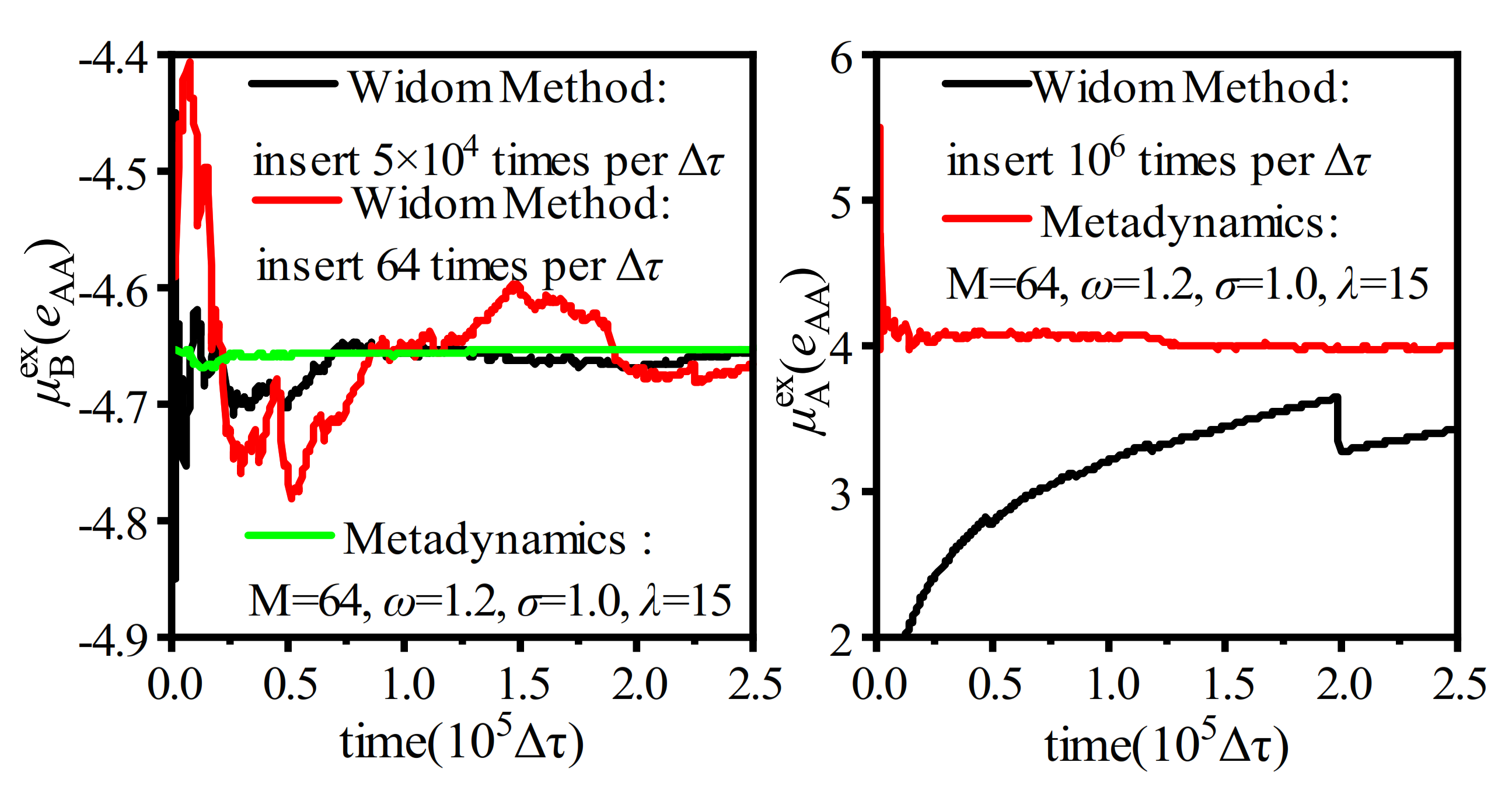
| Khawaja et al. [36] | OPLS | MC: For each of 24 independent systems, selected 250 molecular configurations. Simulated with the Gromacs open source software [39] | Unbiased Widom sampling: 108 times; Volume detection bias: 8 × 10⁴ times |
| Yang et al. [38] | AMBER/OPLS | MC: For each of 20 independent systems, selected 250 molecular configurations | Unbiased Widom sampling: 107 times; Volume detection bias: 2.5 × 10⁵ times |
| T | ρ | μex_W | μex_p | μex_c | μex | μex_R | (μex − μex_R)/μex_R | |
|---|---|---|---|---|---|---|---|---|
| Unit | K | kg/m3 | kcal/mole | kcal/mole | kcal/mole | kcal/mole | kcal/mole | |
| H2O | 315 | 991 | −5.5414 ± 0.083 | −0.0594 | −0.3056 | −5.9064 ± 0.083 | −6.1244 | −3.6% |
| 374 | 958 | −5.2695 ± 0.127 | −0.0574 | −0.036 | −5.3629 ± 0.127 | −5.4828 | −2.2% | |
| 451 | 890 | −4.4862 ± 0.035 | −0.0523 | −0.061 | −4.5995 ± 0.035 | −4.7748 | −3.7% | |
| Ar | 320 | 416 | −0.0222 ± 0.0005 | −0.039 | 0 | −0.0612 ± 0.0005 | −0.0345 | −0.027 |
| 320 | 727 | 0.2176 ± 0.0015 | −0.0681 | 0 | 0.1495 ± 0.0015 | 0.1582 | 5.5% | |
| 320 | 894 | 0.4968 ± 0.0019 | −0.0837 | 0 | 0.4131 ± 0.0019 | 0.3988 | −3.6% |
| Method | Principle | Characteristics | Applicable System/Emulsion Microencapsulation Solution |
|---|---|---|---|
| Original Widom insertion method | Calculating the ensemble-averaged Boltzmann factor, 〈e(−βΔU)〉N using random sampling or uniform grid sampling | For low density systems, the accuracy is acceptable. The calculation is very time-consuming, and the chemical potential accuracy is low for dense systems. | Low-density system |
| Volume detection bias | Inserting of probe particles to evaluate whether the detection area is suitable for particle insertions, and make intensive insertion attempts in the appropriate detected areas | The number of insertions is reduced, the accuracy of the data and the calculation efficiency is effectively improved. Inserting detection particles requires a certain amount of calculation and reasonable evaluation means need to be applied. | Uniform system of medium and high density. Ion/water (W2), alcohol/water (W2), and alkane/aromatics (O) |
| Simulation ensemble bias | The WT-Metadynamics applies additional external potentials to the simulation system to create appropriate insertion positions during the system evolution. Test particles are inserted at specific locations. | The algorithm skillfully constructs low-density regions for particle insertion and dynamically adjusts the system configuration according to the potential energy around the detection point. The implementation is complex. | Uniform or non-uniform complex system. Alkane/aromatics (O), polymer/aromatics (O), and polyalcohol/water (W2) |
| Particle insertion bias | EECM: changing the configuration near the insertion position by repulsing the nearby particles so that the test particle can be inserted successfully; Rosenbluth sampling: inserting of a long-chain molecule segment by segment, and performing of biased sampling based on the change of local internal energy in the growth direction of the chain. | The success rate of a single molecule insertion increases and the number of insertion reduces, but perform a longer time calculation for every insertion. | Dense systems with macromolecular solutes or insoluble solutes. Polymer/aromatics (O) and polyalcohol/water (W2) |
Publisher’s Note: MDPI stays neutral with regard to jurisdictional claims in published maps and institutional affiliations. |
© 2021 by the authors. Licensee MDPI, Basel, Switzerland. This article is an open access article distributed under the terms and conditions of the Creative Commons Attribution (CC BY) license (https://creativecommons.org/licenses/by/4.0/).
Share and Cite
Xu, B.; Liu, X.; Zhou, B. Calculation Methods of Solution Chemical Potential and Application in Emulsion Microencapsulation. Molecules 2021, 26, 2991. https://doi.org/10.3390/molecules26102991
Xu B, Liu X, Zhou B. Calculation Methods of Solution Chemical Potential and Application in Emulsion Microencapsulation. Molecules. 2021; 26(10):2991. https://doi.org/10.3390/molecules26102991
Chicago/Turabian StyleXu, Binkai, Xiangdong Liu, and Bo Zhou. 2021. "Calculation Methods of Solution Chemical Potential and Application in Emulsion Microencapsulation" Molecules 26, no. 10: 2991. https://doi.org/10.3390/molecules26102991
APA StyleXu, B., Liu, X., & Zhou, B. (2021). Calculation Methods of Solution Chemical Potential and Application in Emulsion Microencapsulation. Molecules, 26(10), 2991. https://doi.org/10.3390/molecules26102991