Dissolving Cellulose in 1,2,3-Triazolium- and Imidazolium-Based Ionic Liquids with Aromatic Anions

 ,
,  , , and
Abstract
1. Introduction
2. Results and Discussion
2.1. Physicochemical Properties of the ILs
2.2. Microstructure and Dynamics of the ILs
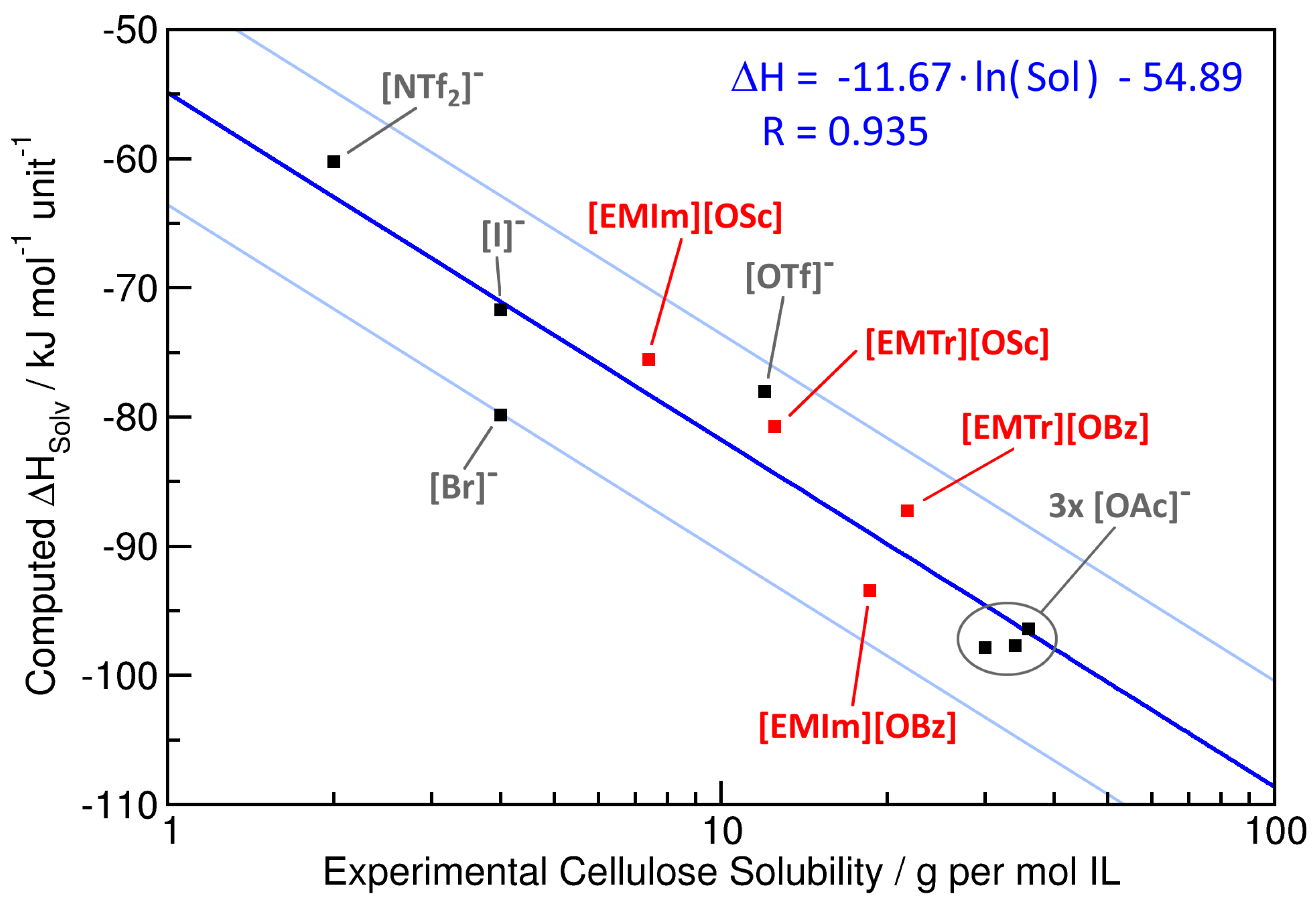
2.3. Cellulose Solubility
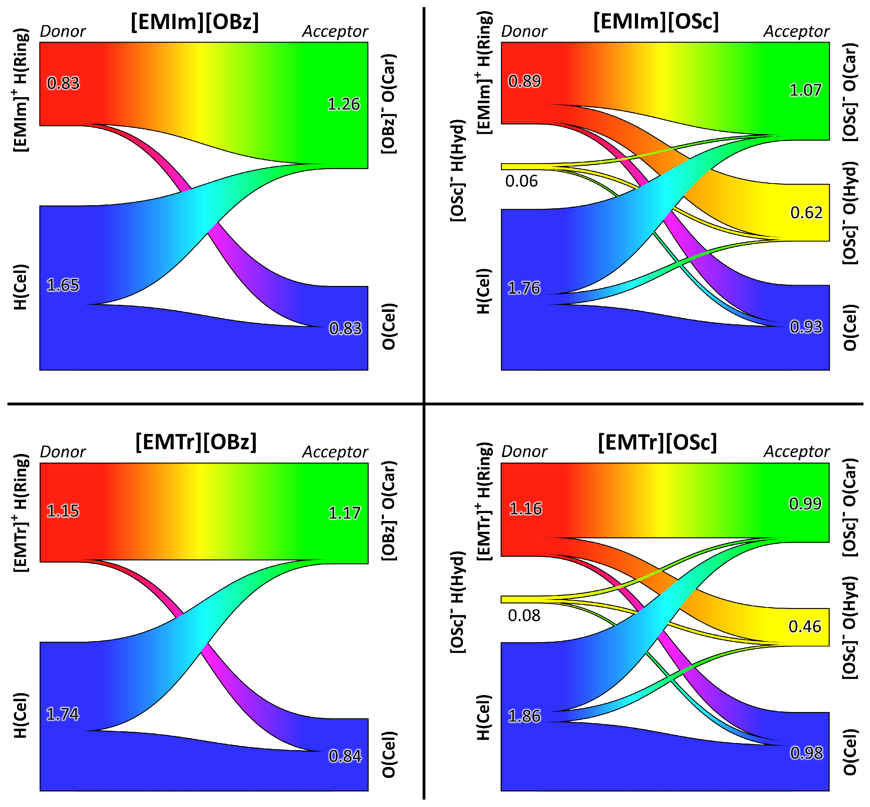
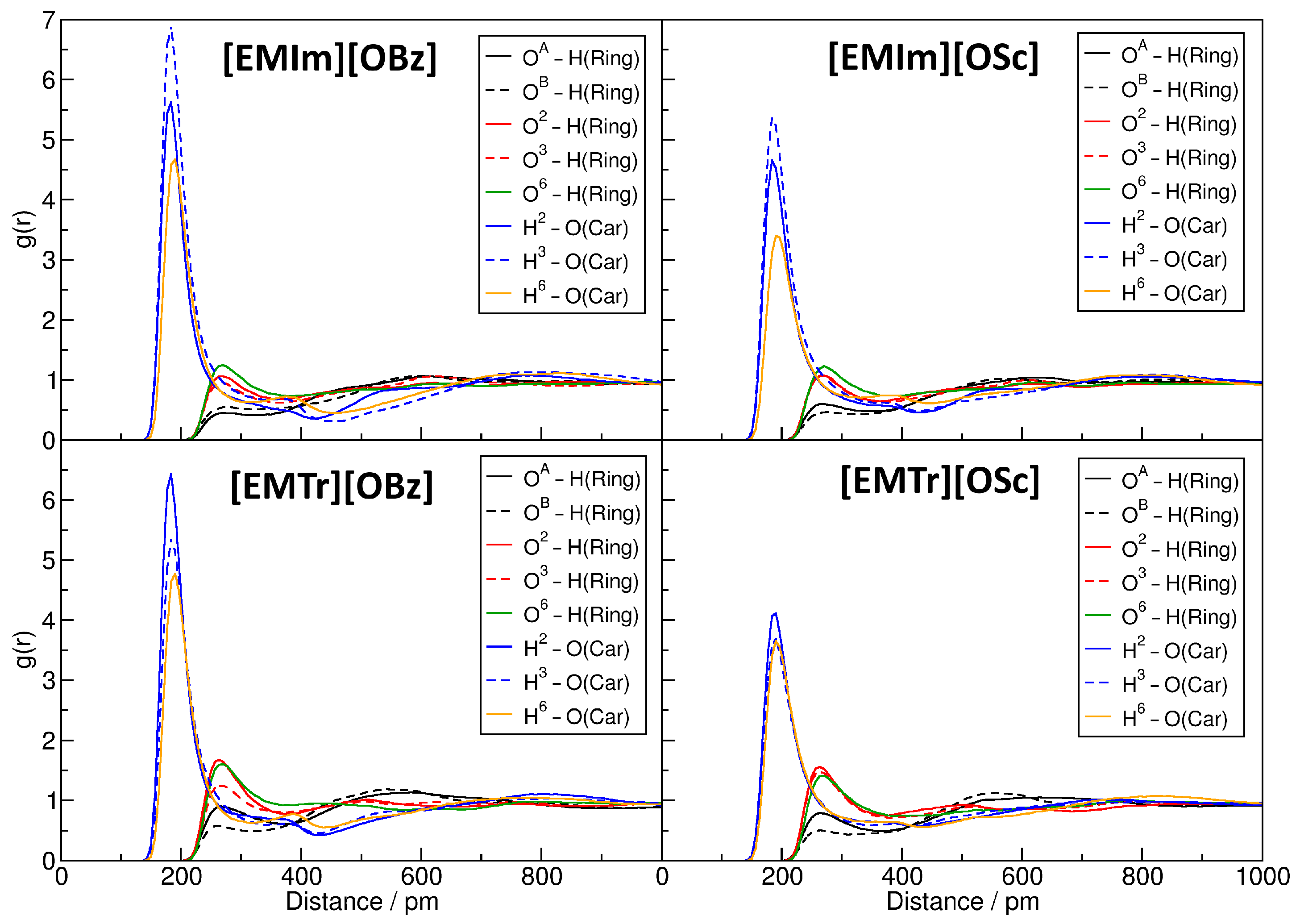
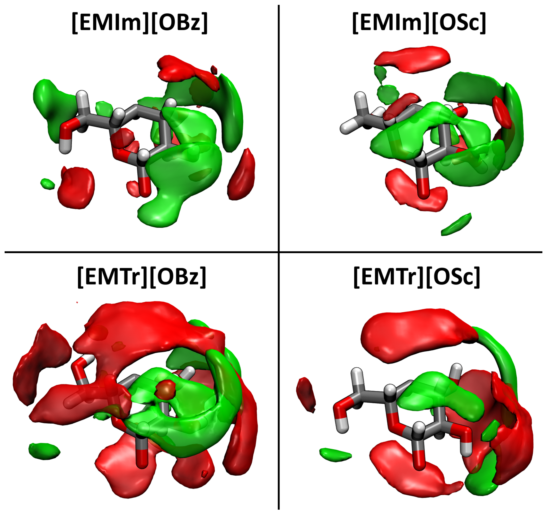
2.4. Microscopic Picture of Cellulose Solvation
3. Materials and Methods
3.1. Experimental Details
3.1.1. Materials
3.1.2. Synthesis
3.1.3. Equipment
3.2. Computational Details
4. Conclusions
Supplementary Materials
Author Contributions
Funding
Acknowledgments
Conflicts of Interest
Abbreviations
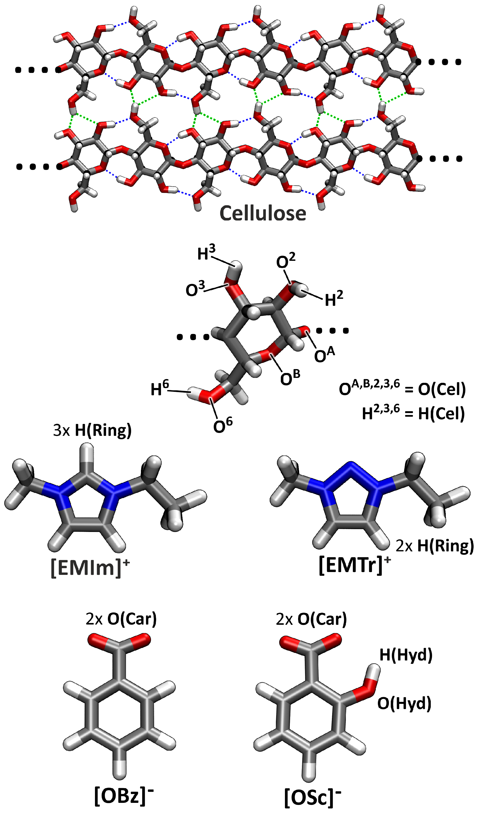
| [EMIm] | 1-Ethyl-3-methylimidazolium cation |
| [EMTr] | 1-Ethyl-3-methyl-1,2,3-triazolium cation |
| [OBz] | Benzoate anion |
| [OSc] | Salicylate anion |
| CL&P | Canongia Lopes & Pádua force field |
| DP | Degree of polymerization |
| FID | Free induction decay |
| IL | Ionic liquid |
| MD | Molecular dynamics |
| MSD | Mean squared displacement |
| NMR | Nuclear magnetic resonance |
| NHC | N-heterocyclic carbenes |
| POM | Polarized optical microscopy |
| PPPM | Particle–particle particle–mesh method |
| RDF | Radial distribution function |
| RESP | Restrained electrostatic potential |
| SDF | Spatial distribution function |
References
- Li, L.; Yi, N.; Wang, X.; Lin, X.; Zeng, T.; Qiu, T. Novel triazolium-based ionic liquids as effective catalysts for transesterification of palm oil to biodiesel. J. Mol. Liq. 2018, 249, 732–738. [Google Scholar] [CrossRef]
- Heinze, T.; El Seoud, O.A.; Koschella, A. Cellulose Derivatives—Synthesis, Structure, and Properties; Springer International Publishing: Cham, Switzerland, 2018. [Google Scholar]
- Cao, Y.; Wu, J.; Zhang, J.; Li, H.; Zhang, Y.; He, J. Room temperature ionic liquids (RTILs): A new and versatile platform for cellulose processing and derivatization. Chem. Eng. J. 2009, 147, 13–21. [Google Scholar] [CrossRef]
- Klass, D.L. Biomass for Renewable Energy, Fuels, and Chemicals; Elsevier: Amsterdam, The Netherlands, 1998. [Google Scholar]
- Zhang, L.; Ruan, D.; Gao, S. Dissolution and regeneration of cellulose in NaOH/thiourea aqueous solution. J. Polym. Sci. Part B Polym. Phys. 2002, 40, 1521–1529. [Google Scholar] [CrossRef]
- Van De Ven, T.G.; Godbout, L. Cellulose: Fundamental Aspects; BoD–Books on Demand: Norderstedt, Germany, 2013. [Google Scholar]
- Watermann, T.; Sebastiani, D. Liquid Water Confined in Cellulose with Variable Interfacial Hydrophilicity. Z. Phys. Chem. 2018, 232, 989–1002. [Google Scholar] [CrossRef]
- Paiva, T.; Echeverria, C.; Godinho, M.H.; Almeida, P.L.; Corvo, M.C. On the influence of imidazolium ionic liquids on cellulose derived polymers. Eur. Polym. J. 2019, 114, 353–360. [Google Scholar] [CrossRef]
- Kostag, M.; Gericke, M.; Heinze, T.; El Seoud, O.A. Twenty-five years of cellulose chemistry: Innovations in the dissolution of the biopolymer and its transformation into esters and ethers. Cellulose 2019, 26, 139–184. [Google Scholar] [CrossRef]
- Swatloski, R.P.; Spear, S.K.; Holbrey, J.D.; Rogers, R.D. Dissolution of Cellose with Ionic Liquids. J. Am. Chem. Soc. 2002, 124, 4974–4975. [Google Scholar] [CrossRef]
- Olsson, C.; Westman, G. Direct dissolution of cellulose: Background, means and applications. Cellul. Fundam. Asp. 2013, 10, 52144. [Google Scholar]
- Payal, R.S.; Bejagam, K.K.; Mondal, A.; Balasubramanian, S. Dissolution of Cellulose in Room Temperature Ionic Liquids: Anion Dependence. J. Phys. Chem. B 2015, 119, 1654–1659. [Google Scholar] [CrossRef]
- Pinkert, A.; Marsh, K.N.; Pang, S.; Staiger, M.P. Ionic Liquids and Their Interaction with Cellulose. Chem. Rev. 2009, 109, 6712–6728. [Google Scholar] [CrossRef]
- Tsuboi, M. Infrared spectrum and crystal structure of cellulose. J. Polym. Sci. 1957, 25, 159–171. [Google Scholar] [CrossRef]
- Yuan, X.; Cheng, G. From cellulose fibrils to single chains: Understanding cellulose dissolution in ionic liquids. Phys. Chem. Chem. Phys. 2015, 17, 31592–31607. [Google Scholar] [CrossRef] [PubMed]
- Walden, P. Molecular weights and electrical conductivity of several fused salts. Bull. Acad. Imper. Sci. 1914, 8, 405–422. [Google Scholar]
- Malberg, F.; Brehm, M.; Hollóczki, O.; Pensado, A.S.; Kirchner, B. Understanding the Evaporation of Ionic Liquids using the Example of 1-Ethyl-3-methylimidazolium Ethylsulfate. Phys. Chem. Chem. Phys. 2013, 15, 18424–18436. [Google Scholar] [CrossRef]
- Sarmiento, G.P.; Zelcer, A.; Espinosa, M.S.; Babay, P.A.; Mirenda, M. Photochemistry of imidazolium cations. Water addition to methylimidazolium ring induced by UV radiation in aqueous solution. J. Photochem. Photobiol. A 2016, 314, 155–163. [Google Scholar] [CrossRef]
- Alpers, T.; Muesmann, T.W.T.; Temme, O.; Christoffers, J. Perfluorinated 1,2,3- and 1,2,4-Triazolium Ionic Liquids. Eur. J. Org. Chem. 2018, 2018, 4331–4337. [Google Scholar] [CrossRef]
- Akbey, Ü.; Granados-Focil, S.; Coughlin, E.B.; Graf, R.; Spiess, H.W. 1H Solid-State NMR Investigation of Structure and Dynamics of Anhydrous Proton Conducting Triazole-Functionalized Siloxane Polymers. J. Phys. Chem. B 2009, 113, 9151–9160. [Google Scholar] [CrossRef]
- Roohi, H.; Salehi, R. Molecular engineering of the electronic, structural, and electrochemical properties of nanostructured 1-methyl-4-phenyl-1, 2, 4-triazolium-based [PhMTZ][X 1–10] ionic liquids through anionic changing. Ionics 2018, 24, 483–504. [Google Scholar] [CrossRef]
- Egorova, K.S.; Seitkalieva, M.M.; Posvyatenko, A.V.; Khrustalev, V.N.; Ananikov, V.P. Cytotoxic Activity of Salicylic Acid-Containing Drug Models with Ionic and Covalent Binding. ACS Med. Chem. Lett. 2015, 6, 1099–1104. [Google Scholar] [CrossRef]
- Pinto, P.C.A.G.; Ribeiro, D.M.G.P.; Azevedo, A.M.O.; Dela Justina, V.; Cunha, E.; Bica, K.; Vasiloiu, M.; Reis, S.; Saraiva, M.L.M.F.S. Active pharmaceutical ingredients based on salicylate ionic liquids: Insights into the evaluation of pharmaceutical profiles. New J. Chem. 2013, 37, 4095–4102. [Google Scholar] [CrossRef]
- Stappert, K.; Ünal, D.; Spielberg, E.T.; Mudring, A.V. Influence of the Counteranion on the Ability of 1-Dodecyl-3-methyltriazolium Ionic Liquids to Form Mesophases. Cryst. Growth Des. 2015, 15, 752–758. [Google Scholar] [CrossRef]
- Parthasarathi, R.; Balamurugan, K.; Shi, J.; Subramanian, V.; Simmons, B.A.; Singh, S. Theoretical Insights into the Role of Water in the Dissolution of Cellulose Using IL/Water Mixed Solvent Systems. J. Phys. Chem. B 2015, 119, 14339–14349. [Google Scholar] [CrossRef] [PubMed]
- Badgujar, K.C.; Bhanage, B.M. Factors governing dissolution process of lignocellulosic biomass in ionic liquid: Current status, overview and challenges. Bioresour. Technol. 2015, 178, 2–18. [Google Scholar] [CrossRef] [PubMed]
- Ries, M.E.; Radhi, A.; Green, S.M.; Moffat, J.; Budtova, T. Microscopic and Macroscopic Properties of Carbohydrate Solutions in the Ionic Liquid 1-Ethyl-3-methyl-imidazolium Acetate. J. Phys. Chem. B 2018, 122, 8763–8771. [Google Scholar] [CrossRef] [PubMed]
- Blasius, J.; Elfgen, R.; Hollóczki, O.; Kirchner, B. Glucose in dry and moist ionic liquid: Vibrational circular dichroism, IR, and possible mechanisms. Phys. Chem. Chem. Phys. 2020, 22, 10726–10737. [Google Scholar] [CrossRef] [PubMed]
- Abdul Sada, A.K.; Greenway, A.M.; Hitchcock, P.B.; Mohammed, T.J.; Seddon, K.R.; Zora, J.A. Upon the structure of room temperature halogenoaluminate ionic liquids. J. Chem. Soc., Chem. Commun. 1986, 1986, 1753–1754. [Google Scholar] [CrossRef]
- Fumino, K.; Wulf, A.; Ludwig, R. Strong, localized, and directional hydrogen bonds fluidize ionic liquids. Angew. Chem. Int. Ed. 2008, 47, 8731–8734. [Google Scholar] [CrossRef]
- Kohagen, M.; Brehm, M.; Thar, J.; Zhao, W.; Müller-Plathe, F.; Kirchner, B. Performance of Quantum Chemically Derived Charges and Persistence of Ion Cages in Ionic Liquids. A Molecular Dynamics Simulations Study of 1-n-Butyl-3-methylimidazolium Bromide. J. Phys. Chem. B 2011, 115, 693–702. [Google Scholar] [CrossRef]
- Kohagen, M.; Brehm, M.; Lingscheid, Y.; Giernoth, R.; Sangoro, J.; Kremer, F.; Naumov, S.; Iacob, C.; Kärger, J.; Valiullin, R.; et al. How Hydrogen Bonds Influence the Mobility of Imidazolium-Based Ionic Liquids. A Combined Theoretical and Experimental Study of 1-n-Butyl-3-methylimidazolium Bromide. J. Phys. Chem. B 2011, 115, 15280–15288. [Google Scholar] [CrossRef]
- Izgorodina, E.I.; MacFarlane, D. Nature of hydrogen bonding in charged hydrogen-bonded complexes and imidazolium-based ionic liquids. J. Phys. Chem. B 2011, 115, 14659–14667. [Google Scholar] [CrossRef]
- Brehm, M.; Weber, H.; Pensado, A.S.; Stark, A.; Kirchner, B. Proton transfer and polarity changes in ionic liquid–water mixtures: A perspective on hydrogen bonds from ab initio molecular dynamics at the example of 1-ethyl-3-methylimidazolium acetate-water mixtures—part 1. Phys. Chem. Chem. Phys. 2012, 14, 5030–5044. [Google Scholar] [CrossRef] [PubMed]
- Pensado, A.S.; Brehm, M.; Thar, J.; Seitsonen, A.P.; Kirchner, B. Effect of Dispersion on the Structure and Dynamics of the Ionic Liquid 1-Ethyl-3-methylimidazolium Thiocyanate. ChemPhysChem 2012, 13, 1845–1853. [Google Scholar] [CrossRef] [PubMed]
- Giernoth, R.; Bröhl, A.; Brehm, M.; Lingscheid, Y. Interactions in Ionic Liquids probed by in situ NMR Spectroscopy. J. Mol. Liq. 2014, 192, 55–58. [Google Scholar] [CrossRef]
- Grøssereid, I.; Lethesh, K.C.; Venkatraman, V.; Fiksdahl, A. New dual functionalized zwitterions and ionic liquids; Synthesis and cellulose dissolution studies. J. Mol. Liq. 2019, 292, 111353. [Google Scholar] [CrossRef]
- Brehm, M.; Pulst, M.; Kressler, J.; Sebastiani, D. Triazolium-Based Ionic Liquids: A Novel Class of Cellulose Solvents. J. Phys. Chem. B 2019, 123, 3994–4003. [Google Scholar] [CrossRef]
- Hollóczki, O.; Firaha, D.S.; Friedrich, J.; Brehm, M.; Cybik, R.; Wild, M.; Stark, A.; Kirchner, B. Carbene formation in ionic liquids: Spontaneous, induced, or prohibited? J. Phys. Chem. B 2013, 117, 5898–5907. [Google Scholar] [CrossRef]
- Finger, L.H.; Guschlbauer, J.; Harms, K.; Sundermeyer, J. N-heterocyclic olefin–carbon dioxide and –sulfur dioxide adducts: Structures and interesting reactivity patterns. Chem. Eur. J. 2016, 22, 16292–16303. [Google Scholar] [CrossRef]
- Rodriguez, H.; Gurau, G.; Holbrey, J.D.; Rogers, R.D. Reaction of elemental chalcogens with imidazolium acetates to yield imidazole-2-chalcogenones: Direct evidence for ionic liquids as proto-carbenes. Chem. Commun. 2011, 47, 3222–3224. [Google Scholar] [CrossRef]
- Singh, D.; Sharma, G.; Gardas, R.L. Better Than the Best Polar Solvent: Tuning the Polarity of 1,2,4- Triazolium-Based Ionic Liquids. ChemistrySelect 2017, 2, 3943–3947. [Google Scholar] [CrossRef]
- Pulst, M.; Golitsyn, Y.; Reichert, D.; Kressler, J. Ion Transport Properties and Ionicity of 1,3-Dimethyl-1,2,3- Triazolium Salts with Fluorinated Anions. Materials 2018, 11, 1723. [Google Scholar] [CrossRef]
- Schulze, B.; Schubert, U.S. Beyond click chemistry—Supramolecular interactions of 1,2,3-triazoles. Chem. Soc. Rev. 2014, 43, 2522–2571. [Google Scholar] [CrossRef] [PubMed]
- Murugesana, S.; Karstb, N.; Islamb, T.; Wienceka, J.M.; Linhardt, R.J. Dialkyl Imidazolium Benzoates—Room Temperature Ionic Liquids Useful in the Peracetylation and Perbenzoylation of Simple and Sulfated Saccharides. Synlett 2003, 9, 1283–1286. [Google Scholar]
- Viswanathan, G.; Murugesan, S.; Pushparaj, V.; Nalamasu, O.; Ajayan, P.M.; Linhardt, R.J. Preparation of Biopolymer Fibers by Electrospinning from Room Temperature Ionic Liquids. Biomacromolecules 2006, 7, 415–418. [Google Scholar] [CrossRef] [PubMed]
- Shekaari, H.; Zafarani-Moattar, M.T.; Mirheydari, S.N. Thermodynamic properties of 1-butyl-3-methylimidazolium salicylate as an active pharmaceutical ingredient ionic liquid (API-IL) in aqueous solutions of glycine and L-alanine at T = (288.15–318.15)K. Thermochim. Acta 2016, 637, 51–68. [Google Scholar] [CrossRef]
- Mitsuzuka, A.; Fujii, A.; Ebata, T.; Mikami, N. Infrared spectroscopy of intramolecular hydrogen-bonded OH stretching vibrations in jet-cooled methyl salicylate and its clusters. J. Phys. Chem. A 1998, 102, 9779–9784. [Google Scholar] [CrossRef]
- Palomar, J.; De Paz, J.L.G.; Catalan, J. Vibrational study of intramolecular hydrogen bonding in o-hydroxybenzoyl compounds. Chem. Phys. 1999, 246, 167–208. [Google Scholar] [CrossRef]
- Stillinger, F. Theoretical Approaches to the Intermolecular Nature of Water. Philos. Trans. R. Soc. B 1977, 278, 97–112. [Google Scholar]
- Rapaport, D. Hydrogen Bonds in Water: Network Organization and Lifetimes. Mol. Phys. 1983, 50, 1151–1162. [Google Scholar] [CrossRef]
- Brehm, M.; Kirchner, B. TRAVIS—A Free Analyzer and Visualizer for Monte Carlo and Molecular Dynamics Trajectories. J. Chem. Inf. Model. 2011, 51, 2007–2023. [Google Scholar] [CrossRef]
- Brehm, M.; Thomas, M.; Gehrke, S.; Kirchner, B. TRAVIS—A Free Analyzer for Trajectories from Molecular Simulation. J. Chem. Phys. 2020, 152, 164105. [Google Scholar] [CrossRef]
- Easteal, A.J.; Price, W.E.; Woolf, L.A. Diaphragm cell for high-temperature diffusion measurements. Tracer Diffusion coefficients for water to 363 K. J. Chem. Soc. Faraday Trans. 1989, 85, 1091–1097. [Google Scholar] [CrossRef]
- Sinnokrot, M.O.; Valeev, E.F.; Sherrill, C.D. Estimates of the ab initio limit for π–π interactions: The benzene dimer. J. Am. Chem. Soc. 2002, 124, 10887–10893. [Google Scholar] [CrossRef] [PubMed]
- Brehm, M.; Weber, H.; Pensado, A.S.; Stark, A.; Kirchner, B. Liquid Structure and Cluster Formation in Ionic Liquid/Water Mixtures—An Extensive ab initio Molecular Dynamics Study on 1-Ethyl-3-Methylimidazolium Acetate/Water Mixtures—Part 2. Z. Phys. Chem. 2013, 227, 177–203. [Google Scholar] [CrossRef]
- Matthews, R.P.; Welton, T.; Hunt, P.A. Hydrogen bonding and π-π interactions in imidazolium-chloride ionic liquid clusters. Phys. Chem. Chem. Phys. 2015, 17, 14437–14453. [Google Scholar] [CrossRef] [PubMed]
- Brehm, M.; Sebastiani, D. Simulating Structure and Dynamics in Small Droplets of 1-Ethyl-3-Methylimidazolium Acetate. J. Chem. Phys. 2018, 148, 193802. [Google Scholar] [CrossRef] [PubMed]
- Wang, H.; Gurau, G.; Rogers, R.D. Ionic liquid processing of cellulose. Chem. Soc. Rev. 2012, 41, 1519–1537. [Google Scholar] [CrossRef]
- Kennedy, A.B.W.; Sankey, H.R. The Thermal Efficiency of Steam Engines. Report of the Committee Appointed to the Council upon the Subject of the Definition of a Standard or Standards of Thermal Efficiency for Steam Engines: With an Introductory Note. (including Appendixes and Plate at Back of Volume). Min. Proc. ICE 1898, 134, 278–312. [Google Scholar]
- Hirose, D.; Wardhana Kusuma, S.B.; Nomura, S.; Yamaguchi, M.; Yasaka, Y.; Kakuchi, R.; Takahashi, K. Effect of anion in carboxylate-based ionic liquids on catalytic activity of transesterification with vinyl esters and the solubility of cellulose. RSC Adv. 2019, 9, 4048–4053. [Google Scholar] [CrossRef]
- Soofivand, F.; Mohandes, F.; Salavati-Niasari, M. Silver chromate and silver dichromate nanostructures: Sonochemical synthesis, characterization, and photocatalytic properties. Mater. Res. Bull. 2013, 48, 2084–2094. [Google Scholar] [CrossRef]
- Plimpton, S. Fast Parallel Algorithms for Short-Range Molecular Dynamics. J. Comp. Phys. 1995, 117, 1–19. [Google Scholar] [CrossRef]
- Martínez, L.; Andrade, R.; Birgin, E.G.; Martínez, J.M. Packmol: A package for building initial configurations for molecular dynamics simulations. J. Comput. Chem. 2009, 30, 2157–2164. [Google Scholar] [CrossRef] [PubMed]
- Canongia Lopes, J.N.; Pádua, A.A.H. Molecular force field for ionic liquids III: Imidazolium, pyridinium, and phosphonium cations; chloride, bromide, and dicyanamide anions. J. Phys. Chem. B 2006, 110, 19586–19592. [Google Scholar] [CrossRef] [PubMed]
- Jorgensen, W.L.; Maxwell, D.S.; Tirado-Rives, J. Development and testing of the OPLS all-atom force field on conformational energetics and properties of organic liquids. J. Am. Chem. Soc. 1996, 118, 11225–11236. [Google Scholar] [CrossRef]
- Bayly, C.I.; Cieplak, P.; Cornell, W.; Kollman, P.A. A well-behaved electrostatic potential based method using charge restraints for deriving atomic charges: The RESP model. J. Phys. Chem. 1993, 97, 10269–10280. [Google Scholar] [CrossRef]
- Damm, W.; Frontera, A.; Tirado-Rives, J.; Jorgensen, W.L. OPLS all-atom force field for carbohydrates. J. Comp. Chem. 1997, 18, 1955–1970. [Google Scholar] [CrossRef]
- Youngs, T.G.A.; Hardacre, C. Application of Static Charge Transfer within an Ionic-Liquid Force Field and Its Effect on Structure and Dynamics. ChemPhysChem 2008, 9, 1548–1558. [Google Scholar] [CrossRef] [PubMed]
- Nose, S. A Unified Formulation of the Constant Temperature Molecular Dynamics Methods. J. Chem. Phys. 1984, 81, 511–519. [Google Scholar] [CrossRef]
- Nose, S. A Molecular Dynamics Method for Simulations in the Canonical Ensemble. Mol. Phys. 1984, 52, 255–268. [Google Scholar] [CrossRef]
- Martyna, G.; Klein, M.; Tuckerman, M. Nosé–Hoover Chains: The Canonical Ensemble via Continuous Dynamics. J. Chem. Phys. 1992, 97, 2635–2643. [Google Scholar] [CrossRef]
- Grace, (c) 1996-2008 Grace Development Team. Available online: http://plasma-gate.weizmann.ac.il/Grace (accessed on 21 March 2020).
- Humphrey, W.; Dalke, A.; Schulten, K. VMD: Visual Molecular Dynamics. J. Mol. Graph. 1996, 14, 33–38. [Google Scholar] [CrossRef]
- Stone, J. An Efficient Library for Parallel Ray Tracing and Animation. Master’s Thesis, Computer Science Department, University of Missouri-Rolla, Rolla, MO, USA, 1998. [Google Scholar]


| Ionic Liquid | Viscosity/Pa s | Density/g cm | State at RT | Water Content/% | Decomp.Temp./°C | ||
|---|---|---|---|---|---|---|---|
| 20 °C | 90 °C | 25 °C | 85 °C | ||||
| [EMIm][OBz] | 0.479 | 0.014 | 1.16 | 1.10 | liquid | 1.27 | 214 |
| [EMIm][OSc] | 0.495 | 0.017 | 1.20 | 1.15 | liquid | 0.65 | 234 |
| [EMTr][OBz] | 0.746 | 0.025 | 1.20 | 1.14 | liquid | 0.87 | 141 |
| [EMTr][OSc] | 1.388 | 0.024 | 1.25 | 1.19 | liquid | 0.33 | 171 |
| Ionic Liquid | Hydrogen Bond Lifetime/ps | |||
|---|---|---|---|---|
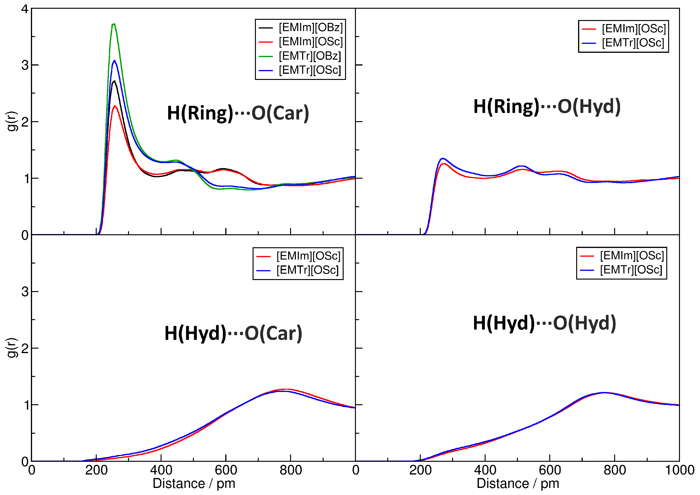
| H(Ring)⋯O(Car) | H(Ring)⋯O(Hyd) | H(Hyd)⋯O(Car) | H(Hyd)⋯O(Hyd) | |
| [EMIm][OBz] | 978 | — | — | — |
| [EMIm][OSc] | 664 | 208 | 22 | 18 |
| [EMTr][OBz] | 1140 | — | — | — |
| [EMTr][OSc] | 797 | 228 | 50 | 29 |
| Ionic Liquid | Self-Diffusion Coefficient/ m s | |
|---|---|---|
| Anion | Cation | |
| [EMIm][OBz] | 97.4 | 61.5 |
| [EMIm][OSc] | 108.9 | 69.6 |
| [EMTr][OBz] | 66.6 | 50.0 |
| [EMTr][OSc] | 74.6 | 52.7 |
| Ionic Liquid | Experimental Cellulose Solubility (80 °C) | Computed /kJ mol unit | Interaction Energy/kJ mol unit | ||
|---|---|---|---|---|---|
| g per mol IL | wt.-% | Cellulose–Anion | Cellulose–Cation | ||
| [EMIm][OBz] | 18.6 | 7.4 | −93.4 | −114.8 | −64.9 |
| [EMIm][OSc] | 7.4 | 2.9 | −75.5 | −105.1 | −68.7 |
| [EMTr][OBz] | 21.7 | 8.5 | −87.3 | −120.7 | −66.5 |
| [EMTr][OSc] | 12.5 | 4.8 | −80.7 | −100.0 | −70.9 |
| Ionic Liquid | Hydrogen Bond Lifetime/ps | ||||
|---|---|---|---|---|---|
| OH(Ring) | OH(Ring) | OH(Ring) | HO(Car) | HO(Car) | |
| [EMIm][OBz] | 1059 | 1186 | 1182 | 10,730 | 2922 |
| [EMIm][OSc] | 709 | 842 | 516 | 3169 | 1288 |
| [EMTr][OBz] | 1320 | 1474 | 976 | 5869 | 4085 |
| [EMTr][OSc] | 2521 | 1783 | 579 | 3088 | 3560 |
© 2020 by the authors. Licensee MDPI, Basel, Switzerland. This article is an open access article distributed under the terms and conditions of the Creative Commons Attribution (CC BY) license (http://creativecommons.org/licenses/by/4.0/).
Share and Cite
Brehm, M.; Radicke, J.; Pulst, M.; Shaabani, F.; Sebastiani, D.; Kressler, J. Dissolving Cellulose in 1,2,3-Triazolium- and Imidazolium-Based Ionic Liquids with Aromatic Anions. Molecules 2020, 25, 3539. https://doi.org/10.3390/molecules25153539
Brehm M, Radicke J, Pulst M, Shaabani F, Sebastiani D, Kressler J. Dissolving Cellulose in 1,2,3-Triazolium- and Imidazolium-Based Ionic Liquids with Aromatic Anions. Molecules. 2020; 25(15):3539. https://doi.org/10.3390/molecules25153539
Chicago/Turabian StyleBrehm, Martin, Julian Radicke, Martin Pulst, Farzaneh Shaabani, Daniel Sebastiani, and Jörg Kressler. 2020. "Dissolving Cellulose in 1,2,3-Triazolium- and Imidazolium-Based Ionic Liquids with Aromatic Anions" Molecules 25, no. 15: 3539. https://doi.org/10.3390/molecules25153539
APA StyleBrehm, M., Radicke, J., Pulst, M., Shaabani, F., Sebastiani, D., & Kressler, J. (2020). Dissolving Cellulose in 1,2,3-Triazolium- and Imidazolium-Based Ionic Liquids with Aromatic Anions. Molecules, 25(15), 3539. https://doi.org/10.3390/molecules25153539