Transport and Optical Gaps in Amorphous Organic Molecular Materials

 ,
,  , , and
Abstract

1. Introduction
2. Methods and Numerical Computations
2.1. General Considerations
2.2. Specific Procedures
3. Results
3.1. Transport Gap
3.2. Optical Gap and Exciton Binding Energies
4. Concluding Remarks
- Calculation of the ground state wave-function and the excitation energy within time independent DFT framework and using high performance combinations of a functional/basis set.
- Incorporate the extended character of the system implemented in the present work by means of a polarized continuum model.
- Our results reveal the importance of considering the exact exchange energy in the calculation of the optimal value of .
Supplementary Materials
Author Contributions
Funding
Acknowledgments
Conflicts of Interest
Abbreviations
| AOM | Amorphous organic materials |
| B3LYP | Hybrid BLYP functional |
| BLYP | Becke-Lee-Yang-Parr exchange correlation functional |
| CAM-B3LYP | Long-range-corrected version of B3LYP functional |
| CT | Charge transferred |
| DFT | Density functional theory |
| EA | Electron affinity |
| GEDT | Global electron density transfer |
| GGA | Generalized gradient approximation |
| G | Fundamental gap |
| G | Transport gap |
| G | Optical gap |
| HOMO | Highest occupied molecular orbital |
| IP | Ionization potential |
| LC-PBE | Long-range-corrected PBE functional |
| LUMO | Lowest unoccupied molecular orbital |
| OLED | Organic light-emitting diode |
| PCM | Polarizable continuum medium |
| PBEPBE | Perdew, Burke and Ernzerhof exchange correlation functional |
| PBE0 | Hybrid PBEPBE functional |
| TD-DFT | Time-dependent DFT |
| HCTH | The -dependent Handy’s functional |
References
- Shirota, Y.; Kageyama, H. Charge carrier transporting molecular materials and their applications in devices. Chem. Rev. 2007, 107, 953–1010. [Google Scholar] [CrossRef] [PubMed]
- Brédas, J.L. Mind the gap! Mater. Horiz. 2014, 1, 17–19. [Google Scholar] [CrossRef]
- Louis, E.; San-Fabián, E.; Díaz-García, M.A.; Chiappe, G.; Vergés, J.A. Are electron affinity and ionization potential intrinsic parameters to predict the electron or hole acceptor character of amorphous molecular materials? J. Phys. Chem. Lett. 2017, 8, 2445–2449. [Google Scholar] [CrossRef] [PubMed]
- Hernández-Verdugo, E.; Sancho-García, J.C.; San-Fabián, E. The application of TD-DFT to excited states of a family of TPD molecules interesting for optoelectronic use. Theor. Chem. Acc. 2017, 136, 77. [Google Scholar] [CrossRef]
- Becke, A.D. Communication: Optical gap in polyacetylene from a simple quantum chemistry exciton model. J. Chem. Phys. 2018, 149, 081102. [Google Scholar] [CrossRef] [PubMed]
- Onida, G.; Reining, L.; Rubio, A. Electronic excitations: Density-functional versus many-body Green’s-function approaches. Rev. Mod. Phys. 2002, 74, 601–659. [Google Scholar] [CrossRef]
- Blase, X.; Attaccalite, C.; Olevano, V. First-principles GW calculations for fullerenes, porphyrins, phtalocyanine, and other molecules of interest for organic photovoltaic applications. Phys. Rev. B 2011, 83, 115103. [Google Scholar] [CrossRef]
- Faber, C.; Boulanger, P.; Attaccalite, C.; Duchemin, I.; Blase, X. Excited states properties of organic molecules: From density functional theory to the GW and Bethe-Salpeter Green’s function formalisms. Philos. Trans. R. Soc. A Math. Phys. Eng. Sci. 2014, 372, 20130271. [Google Scholar] [CrossRef]
- Jacquemin, D.; Duchemin, I.; Blase, X. Is the Bethe–Salpeter formalism accurate for excitation energies? Comparisons with TD-DFT, CASPT2, and EOM-CCSD. J. Phys. Chem. Lett. 2017, 8, 1524–1529. [Google Scholar] [CrossRef]
- Lange, M.F.; Berkelbach, T.C. On the relation between equation-of-motion coupled-cluster theory and the GW approximation. J. Chem. Theory Comput. 2018, 14, 4224–4236. [Google Scholar] [CrossRef]
- Li, J.; D’Avino, G.; Duchemin, I.; Beljonne, D.; Blase, X. Accurate description of charged excitations in molecular solids from embedded many-body perturbation theory. Phys. Rev. B 2018, 97, 035108. [Google Scholar] [CrossRef]
- Duchemin, I.; Jacquemin, D.; Blase, X. Combining the GW formalism with the polarizable continuum model: A state-specific non-equilibrium approach. J. Chem. Phys. 2016, 144, 164106. [Google Scholar] [CrossRef] [PubMed]
- Tomasi, J.; Mennucci, B.; Cammi, R. Quantum mechanical continuum solvation models. Chem. Rev. 2005, 105, 2999–3094. [Google Scholar] [CrossRef] [PubMed]
- Frisch, M.J.; Trucks, G.W.; Schlegel, H.B.; Scuseria, G.E.; Robb, M.A.; Cheeseman, J.R.; Scalmani, G.; Barone, V.; Mennucci, B.; Petersson, G.A.; et al. Gaussian 09 Revision D.01.; Gaussian Inc.: Wallingford, CT, USA, 2009. [Google Scholar]
- Berleb, S.; Brütting, W.; Paasch, G. Interfacial charges and electric field distribution in organic hetero-layer light-emitting devices. Org. Electron. 2000, 1, 41–47. [Google Scholar] [CrossRef]
- Koopmans, T. Über die zuordnung von wellenfunktionen und eigenwerten zu den einzelnen elektronen eines atoms. Physica 1934, 1, 104–113. [Google Scholar] [CrossRef]
- Janak, J.F. Proof that in density-functional theory. Phys. Rev. B 1978, 18, 7165–7168. [Google Scholar] [CrossRef]
- Perdew, J.P.; Parr, R.G.; Levy, M.; Balduz, J.L. Density-functional theory for fractional particle number: Derivative discontinuities of the energy. Phys. Rev. Lett. 1982, 49, 1691–1694. [Google Scholar] [CrossRef]
- Perdew, J.P.; Levy, M. Physical content of the exact kohn-sham orbital energies: Band gaps and derivative discontinuities. Phys. Rev. Lett. 1983, 51, 1884–1887. [Google Scholar] [CrossRef]
- Jones, R.O.; Gunnarsson, O. The density functional formalism, its applications and prospects. Rev. Mod. Phys. 1989, 61, 689–746. [Google Scholar] [CrossRef]
- Levy, M.; Perdew, J.P.; Sahni, V. Exact differential equation for the density and ionization energy of a many-particle system. Phys. Rev. A 1984, 30, 2745–2748. [Google Scholar] [CrossRef]
- Baerends, E.J. Density functional approximations for orbital energies and total energies of molecules and solids. J. Chem. Phys. 2018, 149, 054105. [Google Scholar] [CrossRef] [PubMed]
- Sun, H.; Ryno, S.; Zhong, C.; Ravva, M.K.; Sun, Z.; Körzdörfer, T.; Brédas, J.L. Ionization energies, electron affinities, and polarization energies of organic molecular crystals: Quantitative estimations from a polarizable continuum model (PCM)-tuned range-separated density functional approach. J. Chem. Theory Comput. 2016, 12, 2906–2916. [Google Scholar] [CrossRef] [PubMed]
- Zheng, Z.; Brédas, J.L.; Coropceanu, V. Description of the charge transfer states at the pentacene/C60 interface: Combining range-separated hybrid functionals with the polarizable continuum model. J. Phys. Chem. Lett. 2016, 7, 2616–2621. [Google Scholar] [CrossRef] [PubMed]
- Zheng, Z.; Egger, D.A.; Brédas, J.L.; Kronik, L.; Coropceanu, V. Effect of solid-state polarization on charge-transfer excitations and transport Levels at organic interfaces from a screened range-separated hybrid functional. J. Phys. Chem. Lett. 2017, 8, 3277–3283. [Google Scholar] [CrossRef] [PubMed]
- Nayak, P.K.; Periasamy, N. Calculation of electron affinity, ionization potential, transport gap, optical band gap and exciton binding energy of organic solids using ‘solvation’ model and DFT. Org. Electron. 2009, 10, 1396–1400. [Google Scholar] [CrossRef]
- Tsiper, E.V.; Soos, Z.G. Charge redistribution and polarization energy of organic molecular crystals. Phys. Rev. B 2001, 64, 195124. [Google Scholar] [CrossRef]
- Yoshida, H.; Yamada, K.; Tsutsumi, J.; Sato, N. Complete description of ionization energy and electron affinity in organic solids: Determining contributions from electronic polarization, energy band dispersion, and molecular orientation. Phys. Rev. B 2015, 92, 075145. [Google Scholar] [CrossRef]
- Li, J.; Duchemin, I.; Roscioni, O.M.; Friederich, P.; Anderson, M.; Da Como, E.; Kociok-Köhn, G.; Wenzel, W.; Zannoni, C.; Beljonne, D.; et al. Host dependence of the electron affinity of molecular dopants. Mater. Horiz. 2019, 6, 107–114. [Google Scholar] [CrossRef]
- Schwenn, P.; Burn, P.; Powell, B. Calculation of solid state molecular ionisation energies and electron affinities for organic semiconductors. Org. Electron. 2011, 12, 394–403. [Google Scholar] [CrossRef]
- Madigan, C.; Bulović, V. Exciton energy disorder in polar amorphous organic thin films: Monte Carlo calculations. Phys. Rev. B 2007, 75, 081403. [Google Scholar] [CrossRef]
- Meredith, P.; Bettinger, C.J.; Irimia-Vladu, M.; Mostert, A.B.; Schwenn, P.E. Electronic and optoelectronic materials and devices inspired by nature. Rep. Prog. Phys. 2013, 76, 034501. [Google Scholar] [CrossRef]
- D’Avino, G.; Muccioli, L.; Castet, F.; Poelking, C.; Andrienko, D.; Soos, Z.G.; Cornil, J.; Beljonne, D. Electrostatic phenomena in organic semiconductors: Fundamentals and implications for photovoltaics. J. Phy. Condens. Matter 2016, 28, 433002. [Google Scholar] [CrossRef] [PubMed]
- Stein, T.; Kronik, L.; Baer, R. Reliable prediction of charge transfer excitations in molecular complexes using time-dependent density functional theory. J. Am. Chem. Soc. 2009, 131, 2818–2820. [Google Scholar] [CrossRef]
- Refaely-Abramson, S.; Sharifzadeh, S.; Govind, N.; Autschbach, J.; Neaton, J.B.; Baer, R.; Kronik, L. Quasiparticle spectra from a nonempirical optimally tuned range-separated hybrid density functional. Phys. Rev. Lett. 2012, 109, 226405. [Google Scholar] [CrossRef] [PubMed]
- Kronik, L.; Stein, T.; Refaely-Abramson, S.; Baer, R. Excitation gaps of finite-sized systems from optimally tuned range-separated hybrid functionals. J. Chem. Theory Comput. 2012, 8, 1515–1531. [Google Scholar] [CrossRef] [PubMed]
- Haitao, S.; Jochen, A. Influence of the delocalization error and applicability of optimal functional tuning in density functional calculations of nonlinear optical properties of organic donor-acceptor chromophores. Chem. Phys. Chem. 2013, 14, 2450–2461. [Google Scholar] [CrossRef]
- Becke, A.D. Density-functional exchange-energy approximation with correct asymptotic behavior. Phys. Rev. A 1988, 38, 3098–3100. [Google Scholar] [CrossRef]
- Lee, C.; Yang, W.; Parr, R.G. Development of the Colle-Salvetti correlation-energy formula into a functional of the electron density. Phys. Rev. B 1988, 37, 785–789. [Google Scholar] [CrossRef]
- Perdew, J.P.; Burke, K.; Ernzerhof, M. Generalized gradient approximation made simple. Phys. Rev. Lett. 1996, 77, 3865–3868. [Google Scholar] [CrossRef]
- Perdew, J.P.; Burke, K.; Ernzerhof, M. Erratum: Generalized gradient approximation made simple. Phys. Rev. Lett. 1997, 78, 1396. [Google Scholar] [CrossRef]
- Becke, A.D. Density functional thermochemistry. III. The role of exact exchange. J. Chem. Phys. 1993, 98, 5648–5652. [Google Scholar] [CrossRef]
- Stephens, P.J.; Devlin, F.J.; Chabalowski, C.F.; Frisch, M.J. Ab initio calculation of vibrational absorption and circular dichroism spectra using density functional force fields. J. Phys. Chem. 1994, 98, 11623–11627. [Google Scholar] [CrossRef]
- Adamo, C.; Barone, V. Toward reliable density functional methods without adjustable parameters: The PBE0 model. J. Chem. Phys. 1999, 110, 6158–6170. [Google Scholar] [CrossRef]
- Ernzerhof, M.; Scuseria, G.E. Assessment of the Perdew-Burke-Ernzerhof exchange-correlation functional. J. Chem. Phys. 1999, 110, 5029–5036. [Google Scholar] [CrossRef]
- Boese, A.D.; Handy, N.C. New exchange-correlation density functionals: The role of the kinetic-energy density. J. Chem. Phys. 2002, 116, 9559–9569. [Google Scholar] [CrossRef]
- Schäfer, A.; Horn, H.; Ahlrichs, R. Fully optimized contracted Gaussian basis sets for atoms Li to Kr. J. Chem. Phys. 1992, 97, 2571–2577. [Google Scholar] [CrossRef]
- Weigend, F.; Ahlrichs, R. Balanced basis sets of split valence, triple zeta valence and quadruple zeta valence quality for H to Rn: Design and assessment of accuracy. Phys. Chem. Chem. Phys. 2005, 7, 3297–3305. [Google Scholar] [CrossRef] [PubMed]
- Yanai, T.; Tew, D.P.; Handy, N.C. A new hybrid exchange-correlation functional using the Coulomb-attenuating method (CAM-B3LYP). Chem. Phys. Lett. 2004, 393, 51–57. [Google Scholar] [CrossRef]
- Vydrov, O.A.; Scuseria, G.E. Assessment of a long-range corrected hybrid functional. J. Chem. Phys. 2006, 125, 234109. [Google Scholar] [CrossRef]
- Tsuneda, T.; Song, J.W.; Suzuki, S.; Hirao, K. On Koopmans’ theorem in density functional theory. J. Chem. Phys. 2010, 133, 174101. [Google Scholar] [CrossRef]
- Perdew, J.P.; Yang, W.; Burke, K.; Yang, Z.; Gross, E.K.U.; Scheffler, M.; Scuseria, G.E.; Henderson, T.M.; Zhang, I.Y.; Ruzsinszky, A.; et al. Understanding band gaps of solids in generalized Kohn-Sham theory. Proc. Natl. Acad. Sci. USA 2017, 114, 2801–2806. [Google Scholar] [CrossRef] [PubMed]
- Runge, E.; Gross, E.K.U. Density-functional theory for time-dependent systems. Phys. Rev. Lett. 1984, 52, 997–1000. [Google Scholar] [CrossRef]
- Casida, M.E. Time-dependent density-functional theory for molecules and molecular solids. Theochem-J. Mol. Struct. 2009, 914, 3–18. [Google Scholar] [CrossRef]
- Ullrich, C.A. Time-Dependent Density-Functional Theory: Concepts and Applications; Oxford University Press: Oxford, UK, 2011; p. 536. [Google Scholar]
- Marques, M.A.L.; Maitra, N.T.; Nogueira, F.M.S.; Gross, E.K.U.; Rubio, A. (Eds.) Fundamentals of Time-Dependent Density Functional Theory; Springer: Berlin, Germany, 2012. [Google Scholar]
- Cammi, R.; Mennucci, B. Linear response theory for the polarizable continuum model. Chem. Phys. 1999, 110, 9877–9886. [Google Scholar] [CrossRef]
- Lucke, A.; Ankerhold, J. Dissipative wave-packet dynamics and electron transfer. Chem. Phys. 2001, 115, 4696–4707. [Google Scholar] [CrossRef]
- Shelton, D.P. Ferroelectric domains in nitrobenzene-nitromethane solutions measured by hyper-Rayleigh scattering. Chem. Phys. 2006, 124, 124509. [Google Scholar] [CrossRef] [PubMed]
- Yamamoto, S.; Tatewaki, H.; Watanabe, Y. Gaussian-type function set without prolapse for the Dirac-Fock-Roothaan equation (II): Hg80 through Lr103. Chem. Phys. 2006, 125, 054106. [Google Scholar] [CrossRef] [PubMed]
- Marenich, A.V.; Cramer, C.J.; Truhlar, D.G.; Guido, C.A.; Mennucci, B.; Scalmani, G.; Frisch, M.J. Practical computation of electronic excitation in solution: Vertical excitation model. Chem. Sci. 2011, 2, 2143–2161. [Google Scholar] [CrossRef]
- Jmol. An Open-Source Java Viewer for Chemical Structures in 3D. Available online: http://www.jmol.org (accessed on 8 February 2019).
- Allouche, A.R. Gabedit—A graphical user interface for computational chemistry softwares. J. Comput. Chem. 2011, 32, 174–182. [Google Scholar] [CrossRef]
- Schaftenaar, G.; Noordik, J. Molden: A pre- and post-processing program for molecular and electronic structures. J. Comput.-Aided Mol. Des. 2000, 14, 123–134. [Google Scholar] [CrossRef]
- Lipparini, F.; Scalmani, G.; Mennucci, B.; Cancés, E.; Caricato, M.; Frisch, M.J. A variational formulation of the polarizable continuum model. J. Chem. Phys. 2010, 133, 014106. [Google Scholar] [CrossRef] [PubMed]
- Le Bahers, T.; Adamo, C.; Ciofini, I. A qualitative index of spatial extent in charge-transfer excitations. J. Chem. Theory Comput. 2011, 7, 2498–2506. [Google Scholar] [CrossRef]
- Bässler, H.; Köhler, A. Charge transport in organic semiconductors. In Unimolecular and Supramolecular Electronics I: Chemistry and Physics Meet at Metal-Molecule Interfaces; Metzger, R.M., Ed.; Springer: Berlin/Heidelberg, Germany, 2012; pp. 1–65. [Google Scholar]
- Turkowski, V.; Din, N.U.; Rahman, T.S. Time-dependent density-functional theory and excitons in bulk and two-dimensional semiconductors. Computation 2017, 5, 39. [Google Scholar] [CrossRef]
- Duchemin, I.; Guido, C.A.; Jacquemin, D.; Blase, X. The Bethe–Salpeter formalism with polarisable continuum embedding: Reconciling linear-response and state-specific features. Chem. Sci. 2018, 9, 4430–4443. [Google Scholar] [CrossRef] [PubMed]


| Molecule | E1 | E2 | E3 | H1 | H2 | |||||
| Functional/Basis Set | IP | IP | IP | IP | IP | |||||
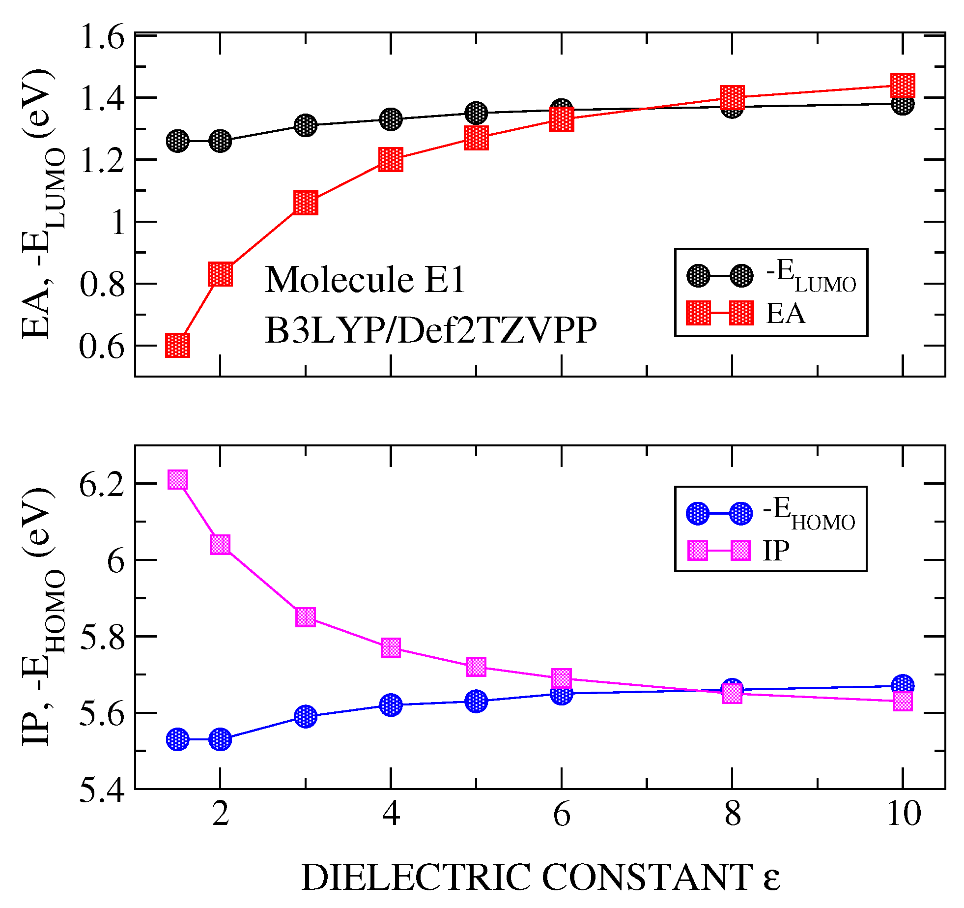
| B3LYP/Def2TZVPP | 7.8 | 5.66 | 9.4 | 6.40 | 9.0 | 6.14 | 8.0 | 5.07 | 8.0 | 5.70 |
| PBE0/Def2TZVPP | 4.6 | 5.78 | 4.8 | 6.55 | 5.0 | 6.36 | 4.7 | 5.22 | 4.8 | 5.86 |
| PBE0/Def2TZV | 4.7 | 5.81 | 4.8 | 6.55 | 5.2 | 6.39 | 4.8 | 5.22 | 5.0 | 5.88 |
| PBE0/Def2SV | 4.9 | 5.79 | 4.8 | 6.55 | 5.5 | 6.39 | 5.0 | 5.25 | 5.2 | 5.91 |
| Molecule | E1 | E2 | E3 | H1 | H2 | |||||
| Functional/Basis Set | EA | EA | EA | EA | EA | |||||
| B3LYP/Def2TZVPP | 7.2 | 1.36 | 8.1 | 1.37 | 8.2 | 1.78 | 8.1 | 1.28 | 8.4 | 1.52 |
| PBE0/Def2TZVPP | 4.7 | 1.16 | 4.8 | 1.13 | 4.4 | 1.59 | 4.6 | 1.12 | 4.9 | 1.38 |
| PBE0/Def2TZV | 4.7 | 1.10 | 4.8 | 1.19 | 4.8 | 1.69 | 4.8 | 1.02 | 5.2 | 1.29 |
| PBE0/Def2SV | 5.0 | 1.08 | 5.1 | 1.12 | 5.0 | 1.64 | 5.0 | 1.12 | 5.6 | 1.43 |
| No. | Molecule | (eV) | Oscillator Strength |
|---|---|---|---|
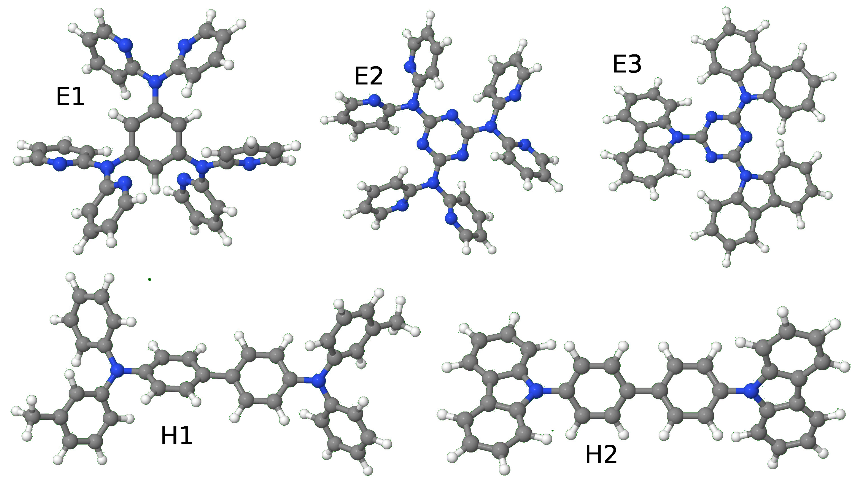
| E1 | 1,3,5-tris(phenyl-2-pyridylamino)benzene | 3.745 | 0.024 |
| 3.891 | 0.094 | ||
| 3.944 | 0.211 | ||
| 4.026 | 0.023 | ||
| E2 | 2,4,6-tris[di(2-pyridyl)-amino]-1,3,5-triazine | 4.480 | 0.207 |
| 4.511 | 0.352 | ||
| 4.525 | 0.226 | ||
| 4.646 | 0.092 | ||
| E3 | 2,4,6-tris(carbazolo)-1,3,5-triazine (TRZ2) | 3.911 | 0.326 |
| 4.023 | 0.011 | ||
| 4.040 | 0.421 | ||
| 4.149 | 0.015 | ||
| H1 | N,N′-Bis(3-methylphenyl)-N,N′-diphenylbenzidine (TPD) | 3.405 | 1.122 |
| 3.655 | 0.000 | ||
| 3.738 | 0.025 | ||
| 3.910 | 0.001 | ||
| H2 | 4,4′-di(N-carbazolyl)biphenyl (CBP) | 3.772 | 0.714 |
| 3.974 | 0.000 | ||
| 3.999 | 0.093 | ||
| 4.018 | 0.000 |
| Molecule | Excited State | (eV) | Oscillator Strength |
|---|---|---|---|
| E1 | 2 | 3.807 | 0.116 |
| E2 | 2 | 4.505 | 0.354 |
| E3 | 1 | 3.752 | 0.301 |
| H1 | 1 | 3.373 | 1.109 |
| H2 | 1 | 3.604 | 0.632 |
| Molecule | IP | IP | EA | ||||||
|---|---|---|---|---|---|---|---|---|---|
| E1 | 5.09 | 3.45 | 1.64 | 4.62 | 5.78 | 1.16 | 4.62 | 3.81 | 0.81 |
| E2 | 5.07 | 3.72 | 1.35 | 4.80 | 6.56 | 1.14 | 5.42 | 4.50 | 0.92 |
| E3 | 6.0 | 3.4 | 2.60 | 4.72 | 6.37 | 1.56 | 4.81 | 3.75 | 1.06 |
| H1 | 5.50 | 3.2 | 2.3 | 4.65 | 5.23 | 1.13 | 4.1 | 3.37 | 0.73 |
| H2 | 6.3 | 3.1 | 3.2 | 4.88 | 5.87 | 1.39 | 4.48 | 3.60 | 0.88 |
| Molecule | Excited State | (Electron-Charge) | (Å) | (Debye) |
|---|---|---|---|---|
| E1 | 2 | 0.768 | 1.915 | 7.068 |
| E2 | 2 | 0.472 | 0.571 | 1.293 |
| E3 | 1 | 0.832 | 2.400 | 9.597 |
| H1 | 1 | 0.572 | 0.396 | 1.088 |
| H2 | 1 | 0.857 | 0.014 | 0.056 |
© 2019 by the authors. Licensee MDPI, Basel, Switzerland. This article is an open access article distributed under the terms and conditions of the Creative Commons Attribution (CC BY) license (http://creativecommons.org/licenses/by/4.0/).
Share and Cite
San-Fabián, E.; Louis, E.; Díaz-García, M.A.; Chiappe, G.; Vergés, J.A. Transport and Optical Gaps in Amorphous Organic Molecular Materials. Molecules 2019, 24, 609. https://doi.org/10.3390/molecules24030609
San-Fabián E, Louis E, Díaz-García MA, Chiappe G, Vergés JA. Transport and Optical Gaps in Amorphous Organic Molecular Materials. Molecules. 2019; 24(3):609. https://doi.org/10.3390/molecules24030609
Chicago/Turabian StyleSan-Fabián, Emilio, Enrique Louis, María A. Díaz-García, Guillermo Chiappe, and José A. Vergés. 2019. "Transport and Optical Gaps in Amorphous Organic Molecular Materials" Molecules 24, no. 3: 609. https://doi.org/10.3390/molecules24030609
APA StyleSan-Fabián, E., Louis, E., Díaz-García, M. A., Chiappe, G., & Vergés, J. A. (2019). Transport and Optical Gaps in Amorphous Organic Molecular Materials. Molecules, 24(3), 609. https://doi.org/10.3390/molecules24030609