
Machine Learning Approaches for Protein–Protein Interaction Hot Spot Prediction: Progress and Comparative Assessment


Abstract
1. Introduction
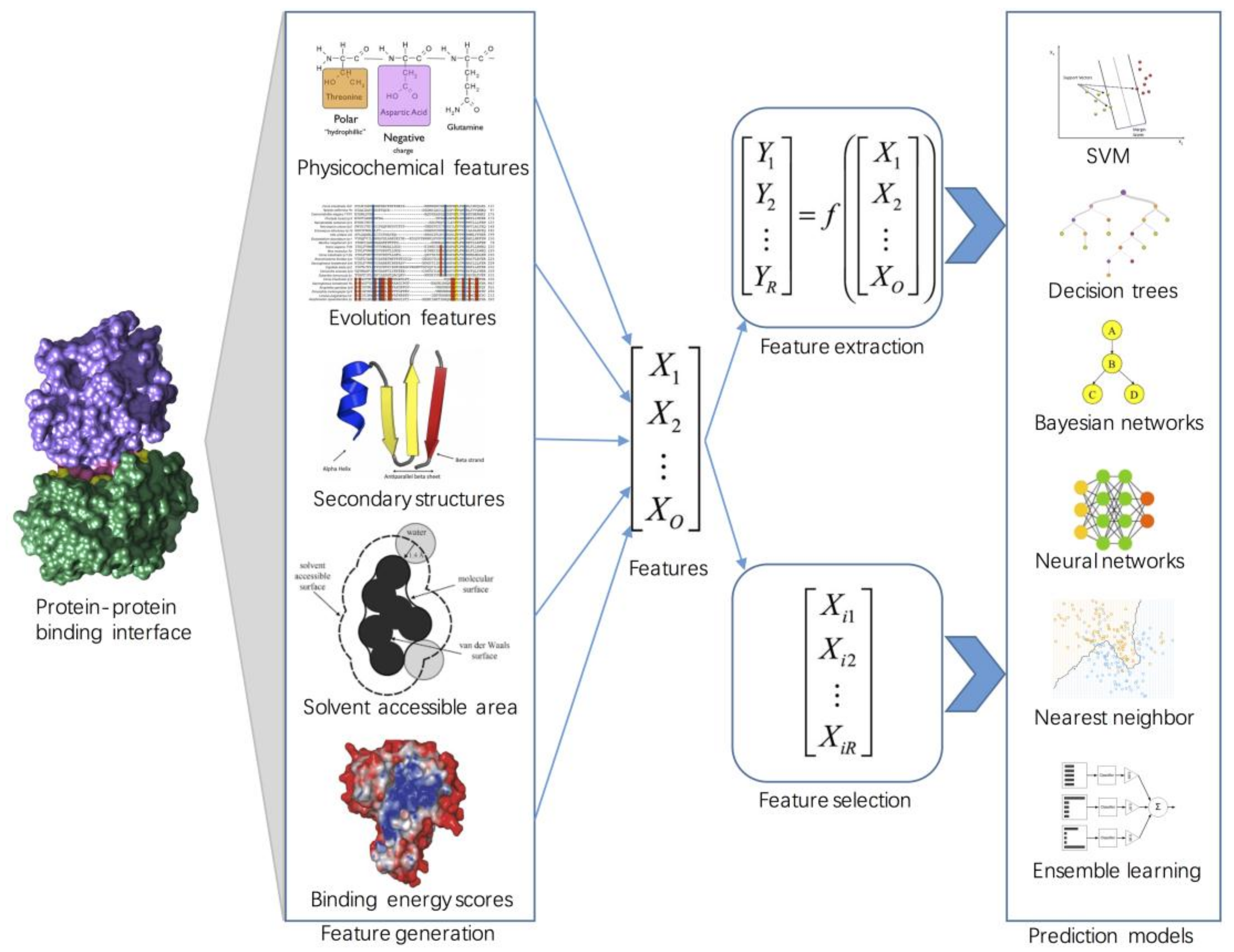
2. Feature Engineering
2.1. Sequence-Based Features
2.2. Structure-Based Features
2.3. Energy-Based Features
2.4. Feature Selection
2.5. Feature Extraction
3. Machine Learning Approaches for Hot Spot Prediction
3.1. Nearest Neighbor
3.2. Support Vector Machines
3.3. Decision Trees
3.4. Bayesian Networks
3.5. Neural Networks
3.6. Ensemble Learning
4. Comparative Assessment
4.1. Datasets
4.2. Performance Measures
4.3. Performance Evaluation of Different Features
4.4. Performance Comparison of Existing Hot Spot Prediction Methods
5. Discussion
- (1)
- Hot spots are mainly discovered through biological experiments, lacking mature theoretical support and unified identification standards. Although the O-ring theory [9] with great influence explains the arrangement relationship between energy hot spots and surrounding residues well, it still has much controversy; the change of free energy (∆∆G) is usually used to discriminate energy hot spots, but different articles use different thresholds under different conditions, and they lack uniform standards.
- (2)
- Systematic mutagenesis experiments are currently expensive and time-consuming to perform; the experimental data of energy hot spots are very limited, resulting in a lack of large benchmark datasets. As we observed in this study, supervised learning methods, especially GTB, have achieved good results, but the performance of each 10-fold cross-validation varies on repetition. Alternatively, semi-supervised learning and transductive inference approaches can be used to take advantage of the large number of unlabeled data to further improve the predictive performance.
- (3)
- Due to the small number of samples and the large number of features in hot spot prediction, machine learning methods are easy to overfit. Improved feature extraction methods and feature selection approaches can help avoid overfitting. At the same time, the number of hot spots is far less than the number of non-hot spots, leading to the so-called imbalance problem. It is necessary to design effective algorithms (e.g. ensemble learning) to solve this problem.
- (4)
- The characteristics of accurately identifying energy hot spots have not been well discovered, and no single feature can fully identify energy hot spots from the interface residues. This requires finding new and effective features, and studying the effects of combining different categories of features. For example, most existing machine learning hot spot predictors use statistical sequence and structural information to encode input feature vectors, but the spatial arrangement of residues has not been well exploited.
- (5)
- Molecular dynamics simulation and molecular docking techniques can simulate the changes in binding free energy before and after alanine mutation. A promising future direction is developing effective ways to combine computational docking with machine learning methods, which has the potential to dramatically boost hot spot predictions.
Author Contributions
Funding
Acknowledgments
Conflicts of Interest
References
- Zeng, J.; Li, D.; Wu, Y.; Zou, Q.; Liu, X. An empirical study of features fusion techniques for protein-protein interaction prediction. Curr. Bioinform. 2016, 11, 4–12. [Google Scholar] [CrossRef]
- Moreira, I.S.; Fernandes, P.A.; Ramos, M.J. Hot spots—A review of the protein–protein interface determinant amino-acid residues. Proteins Struct. Funct. Bioinform. 2007, 68, 803–812. [Google Scholar] [CrossRef] [PubMed]
- Xia, J.; Yue, Z.; Di, Y.; Zhu, X.; Zheng, C.H. Predicting hot spots in protein interfaces based on protrusion index, pseudohydrophobicityandelectron-ioninteractionpseudopotentialfeatures. Oncotarget 2016, 7, 18065–18075. [Google Scholar] [CrossRef] [PubMed]
- Thorn, K.S.; Bogan, A.A. ASEdb: A database of alanine mutations and their effects on the free energy of binding in protein interactions. Bioinformatics 2001, 17, 284–285. [Google Scholar] [CrossRef] [PubMed]
- Fischer, T.; Arunachalam, K.; Bailey, D.; Mangual, V.; Bakhru, S.; Russo, R.; Huang, D.; Paczkowski, M.; Lalchandani, V.; Ramachandra, C.; et al. The binding interface database (BID): a compilation of amino acid hot spots in protein interfaces. Bioinformatics 2003, 19, 1453–1454. [Google Scholar] [CrossRef] [PubMed]
- Kumar, M.S.; Gromiha, M.M. PINT: protein–protein interactions thermodynamic database. Nucleic Acids Res. 2006, 34, D195–D198. [Google Scholar] [CrossRef] [PubMed]
- Moal, I.H.; Fernández-Recio, J. SKEMPI: A Structural Kinetic and Energetic database of Mutant Protein Interactions and its use in empirical models. Bioinformatics 2012, 28, 2600–2607. [Google Scholar] [CrossRef] [PubMed]
- Li, X.; Keskin, O.; Ma, B.; Nussinov, R.; Liang, J. Protein-Protein Interactions: Hot Spots and Structurally Conserved Residues often Locate in Complemented Pockets that Pre-organized in the Unbound States: Implications for Docking. J. Mol. Boil. 2004, 344, 781–795. [Google Scholar] [CrossRef] [PubMed]
- Clackson, T.; Wells, J.A. A hot spot of binding energy in a hormone-receptor interface. Science 1995, 267, 383–386. [Google Scholar] [CrossRef] [PubMed]
- Li, J.; Liu, Q. ‘Double water exclusion’: A hypothesis refining the O-ring theory for the hot spots at protein interfaces. Bioinformatics 2009, 25, 743–750. [Google Scholar] [CrossRef] [PubMed]
- Deng, L.; Guan, J.; Wei, X.; Yi, Y.; Zhang, Q.C.; Zhou, S. Boosting prediction performance of protein-protein interaction hot spots by using structural neighborhood properties. J. Comput. Biol. 2013, 20, 878. [Google Scholar] [CrossRef] [PubMed]
- Deng, L.; Guan, J.; Dong, Q.; Zhou, S. Prediction of protein-protein interaction sites using an ensemble method. BMC Bioinform. 2009, 10, 426. [Google Scholar] [CrossRef] [PubMed]
- Deng, L.; Fan, C.; Zeng, Z. A sparse autoencoder-based deep neural network for protein solvent accessibility and contact number prediction. BMC Bioinform. 2017, 18, 569. [Google Scholar] [CrossRef] [PubMed]
- Kawashima, S.; Pokarowski, P.; Pokarowska, M.; Kolinski, A.; Katayama, T.; Kanehisa, M. AAindex: Amino acid index database, progress report 2008. Nucleic Acids Res. 2007, 36, D202–D205. [Google Scholar] [CrossRef] [PubMed]
- Chen, P.; Li, J.; Wong, L.; Kuwahara, H.; Huang, J.Z.; Gao, X. Accurate prediction of hot spot residues through physicochemical characteristics of amino acid sequences. Proteins Struct. Funct. Bioinform. 2013, 81, 1351–1362. [Google Scholar] [CrossRef] [PubMed]
- Jiang, J.; Wang, N.; Chen, P.; Zheng, C.; Wang, B. Prediction of Protein Hotspots from Whole Protein Sequences by a Random Projection Ensemble System. Int. J. Mol. Sci. 2017, 18, 1543. [Google Scholar] [CrossRef] [PubMed]
- Altschul, S.F.; Madden, T.L.; Schäffer, A.A.; Zhang, J.; Zhang, Z.; Miller, W.; Lipman, D.J. Gapped BLAST and PSI-BLAST: A New Generation of Protein Database Search Programs. Nucleic Acids Res. 1997, 25, 3389–3402. [Google Scholar] [CrossRef] [PubMed]
- Melo, R.; Fieldhouse, R.; Melo, A.; Correia, J.D.; Cordeiro, M.N.D.; Gümüş, Z.H.; Costa, J.; Bonvin, A.M.; Moreira, I.S. A machine learning approach for hot-spot detection at protein-protein interfaces. Int. J. Mol. Sci. 2016, 17, 1215. [Google Scholar] [CrossRef] [PubMed]
- Moreira, I.S.; Koukos, P.I.; Melo, R.; Almeida, J.G.; Preto, A.J.; Schaarschmidt, J.; Trellet, M.; Gümüs, Z.H.; Costa, J.; Bonvin, A.M. SpotOn: High Accuracy Identification of Protein-Protein Interface Hot-Spots. Sci. Rep. 2017, 7, 8007. [Google Scholar] [CrossRef] [PubMed]
- Chan, C.H.; Liang, H.K.; Hsiao, N.W.; Ko, M.T.; Lyu, P.C.; Hwang, J.K. Relationship between local structural entropy and protein thermostabilty. Proteins Struct. Funct. Bioinform. 2004, 57, 684–691. [Google Scholar] [CrossRef] [PubMed]
- Pan, Y.; Wang, Z.; Zhan, W.; Deng, L. Computational identification of binding energy hot spots in protein-RNA complexes using an ensemble approach. Bioinformatics 2017, 34, 1473–1480. [Google Scholar] [CrossRef] [PubMed]
- Ashkenazy, H.; Erez, E.; Martz, E.; Pupko, T.; Ben-Tal, N. ConSurf 2010: calculating evolutionary conservation in sequence and structure of proteins and nucleic acids. Nucleic Acids Res. 2010, 38, W529–W533. [Google Scholar] [CrossRef] [PubMed]
- Higa, R.H.; Tozzi, C.L. Prediction of binding hot spot residues by using structural and evolutionary parameters. Genet. Mol. Boil. 2009, 32, 626–633. [Google Scholar] [CrossRef] [PubMed]
- Shingate, P.; Manoharan, M.; Sukhwal, A.; Sowdhamini, R. ECMIS: computational approach for the identification of hotspots at protein-protein interfaces. BMC Bioinform. 2014, 15, 303. [Google Scholar] [CrossRef] [PubMed]
- Joosten, R.P.; Te Beek, T.A.; Krieger, E.; Hekkelman, M.L.; Hooft, R.W.; Schneider, R.; Sander, C.; Vriend, G. A series of PDB related databases for everyday needs. Nucleic Acids Res. 2010, 9, D411–D419. [Google Scholar] [CrossRef] [PubMed]
- Lee, B.; Richards, F.M. The interpretation of protein structures: estimation of static accessibility. J. Mol. Boil. 1971, 55, 379–IN4. [Google Scholar] [CrossRef]
- Tuncbag, N.; Gursoy, A.; Keskin, O. Identification of computational hot spots in protein interfaces: combining solvent accessibility and inter-residue potentials improves the accuracy. Bioinformatics 2009, 25, 1513–20. [Google Scholar] [CrossRef] [PubMed]
- Xia, J.F.; Zhao, X.M.; Song, J.; Huang, D.S. APIS: accurate prediction of hot spots in protein interfaces by combining protrusion index with solvent accessibility. BMC Bioinform. 2010, 11, 174. [Google Scholar] [CrossRef] [PubMed]
- Keskin, O.; Ma, B.; Nussinov, R. Hot regions in protein–protein interactions: the organization and contribution of structurally conserved hot spot residues. J. Mol. Boil. 2005, 345, 1281–1294. [Google Scholar] [CrossRef] [PubMed]
- Cho, K.i.; Kim, D.; Lee, D. A feature-based approach to modeling protein–protein interaction hot spots. Nucleic Acids Res. 2009, 37, 2672–2687. [Google Scholar] [CrossRef] [PubMed]
- Darnell, S.J.; Page, D.; Mitchell, J.C. An automated decision-tree approach to predicting protein interaction hot spots. Proteins Struct. Funct. Bioinform. 2007, 68, 813–823. [Google Scholar] [CrossRef] [PubMed]
- Liang, S.; Grishin, N.V. Effective scoring function for protein sequence design. Proteins Struct. Funct. Bioinform. 2004, 54, 271–281. [Google Scholar] [CrossRef] [PubMed]
- Lee, D.T.; Schachter, B.J. Two algorithms for constructing a Delaunay triangulation. Int. J. Comput. Inf. Sci. 1980, 9, 219–242. [Google Scholar] [CrossRef]
- Deng, L.; Zhang, Q.C.; Chen, Z.; Meng, Y.; Guan, J.; Zhou, S. PredHS: A web server for predicting protein–protein interaction hot spots by using structural neighborhood properties. Nucleic Acids Res. 2014, 42, W290–W295. [Google Scholar] [CrossRef] [PubMed]
- Kortemme, T.; Kim, D.E.; Baker, D. Computational alanine scanning of protein-protein interfaces. Sci. STKE 2004, pl2. [Google Scholar] [CrossRef] [PubMed]
- Tuncbag, N.; Keskin, O.; Gursoy, A. HotPoint: Hot spot prediction server for protein interfaces. Nucleic Acids Res. 2010, 38, W402–W406. [Google Scholar] [CrossRef] [PubMed]
- Lise, S.; Archambeau, C.; Pontil, M.; Jones, D.T. Prediction of hot spot residues at protein-protein interfaces by combining machine learning and energy-based methods. BMC Bioinform. 2009, 10, 365. [Google Scholar] [CrossRef] [PubMed]
- Lise, S.; Buchan, D.; Pontil, M.; Jones, D.T. Predictions of hot spot residues at protein-protein interfaces using support vector machines. PLoS ONE 2011, 6, e16774. [Google Scholar] [CrossRef] [PubMed]
- Liang, S.; Meroueh, S.O.; Wang, G.; Qiu, C.; Zhou, Y. Consensus scoring for enriching near-native structures from protein–protein docking decoys. Proteins Struct. Funct. Bioinform. 2009, 75, 397. [Google Scholar] [CrossRef] [PubMed]
- Saeys, Y.; Inza, I.; Larrañaga, P. A review of feature selection techniques in bioinformatics. Bioinformatics 2007, 23, 2507–2517. [Google Scholar] [CrossRef] [PubMed]
- Chen, Y.W.; Lin, C.J. Combining SVMs with various feature selection strategies. In Feature Extraction; Springer: Berlin, Germany, 2006; pp. 315–324. [Google Scholar]
- Breiman, L. Random forests. Mach. Learn. 2001, 45, 5–32. [Google Scholar] [CrossRef]
- Guyon, I.; Weston, J.; Barnhill, S.; Vapnik, V. Gene selection for cancer classification using support vector machines. Mach. Learn. 2002, 46, 389–422. [Google Scholar] [CrossRef]
- Peng, H.; Long, F.; Ding, C. Feature selection based on mutual information criteria of max-dependency, max-relevance, and min-redundancy. IEEE Trans. Pattern Anal. Mach. Intell. 2005, 27, 1226–1238. [Google Scholar] [CrossRef] [PubMed]
- Wang, S.P.; Zhang, Q.; Lu, J.; Cai, Y.D. Analysis and prediction of nitrated tyrosine sites with the mRMR method and support vector machine algorithm. Curr. Bioinform. 2018, 13, 3–13. [Google Scholar] [CrossRef]
- Zou, Q.; Zeng, J.; Cao, L.; Ji, R. A novel features ranking metric with application to scalable visual and bioinformatics data classification. Neurocomputing 2016, 173, 346–354. [Google Scholar] [CrossRef]
- Wang, L.; Zhang, W.; Gao, Q.; Xiong, C. Prediction of hot spots in protein interfaces using extreme learning machines with the information of spatial neighbour residues. IET Syst. Boil. 2014, 8, 184–190. [Google Scholar] [CrossRef] [PubMed]
- Qiao, Y.; Xiong, Y.; Gao, H.; Zhu, X.; Chen, P. Protein-protein interface hot spots prediction based on a hybrid feature selection strategy. BMC Bioinform. 2018, 19, 14. [Google Scholar] [CrossRef] [PubMed]
- Wold, S.; Esbensen, K.; Geladi, P. Principal component analysis. Chemom. Intell. Lab. Syst. 1987, 2, 37–52. [Google Scholar] [CrossRef]
- Jia, C.; Zuo, Y.; Zou, Q. O-GlcNAcPRED-II: An integrated classification algorithm for identifying O-GlcNAcylation sites based on fuzzy undersampling and a K-means PCA oversampling technique. Bioinformatics 2018, 34, 2029–2036. [Google Scholar] [CrossRef] [PubMed]
- Mika, S.; Ratsch, G.; Weston, J.; Scholkopf, B.; Mullers, K.R. Fisher discriminant analysis with kernels. Neural networks for signal processing IX, 1999. In Proceedings of the 1999 IEEE Signal Processing Society Workshop, 1999; 1999; pp. 41–48. [Google Scholar]
- Cover, T.M. Nearest Neighbour Pattern Classification. IEEE Trans. Inf. Theory 1967, 13, 21–27. [Google Scholar] [CrossRef]
- Cortes, C.; Vapnik, V. Support-vector networks. Mach. Learn. 1995, 20, 273–297. [Google Scholar] [CrossRef]
- Quinlan, J.R. Induction on decision tree. Mach. Learn. 1986, 1, 81–106. [Google Scholar] [CrossRef]
- Friedman, N.; Dan, G.; Goldszmidt, M. Bayesian Network Classifiers. Mach. Learn. 1997, 29, 131–163. [Google Scholar] [CrossRef]
- Yao, X. Evolving artificial neural networks. Proc. IEEE 1999, 87, 1423–1447. [Google Scholar]
- Wan, S.; Duan, Y.; Zou, Q. HPSLPred: An ensemble multi-label classifier for human protein subcellular location prediction with imbalanced source. Proteomics 2017, 17, 1700262. [Google Scholar] [CrossRef] [PubMed]
- Hu, S.S.; Chen, P.; Wang, B.; Li, J. Protein binding hot spots prediction from sequence only by a new ensemble learning method. Amino Acids 2017, 49, 1–13. [Google Scholar] [CrossRef] [PubMed]
- Ye, L.; Kuang, Q.; Jiang, L.; Luo, J.; Jiang, Y.; Ding, Z.; Li, Y.; Li, M. Prediction of hot spots residues in protein–protein interface using network feature and microenvironment feature. Chemom. Intell. Lab. Syst. 2014, 131, 16–21. [Google Scholar] [CrossRef]
- Zhu, X.; Mitchell, J.C. KFC2: A knowledge-based hot spot prediction method based on interface solvation, atomic density, and plasticity features. Proteins Struct. Funct. Bioinform. 2011, 79, 2671–2683. [Google Scholar] [CrossRef] [PubMed]
- Quinlan, J.R. C4. 5: Programs for Machine Learning; Elsevier: New York, NY, USA, 2014. [Google Scholar]
- Andersen, S.K. Judea Pearl, Probabilistic Reasoning in Intelligent Systems: Networks of Plausible Inference. Artif. Intell. 1991, 48, 117–124. [Google Scholar] [CrossRef]
- Irwin, M. Learning in Graphical Models; Kluwer Academic Publishers: Dordrecht, The Netherlands, 1998; pp. 140–155. [Google Scholar]
- Domingos, P.; Pazzani, M. On the Optimality of the Simple Bayesian Classifier under Zero-One Loss; Kluwer Academic Publishers: Dordrecht, The Netherlands, 1997. [Google Scholar]
- Assi, S.A.; Tanaka, T.; Rabbitts, T.H.; Fernandezfuentes, N. PCRPi: Presaging Critical Residues in Protein interfaces, a new computational tool to chart hot spots in protein interfaces. Nucleic Acids Res. 2010, 38, e86. [Google Scholar] [CrossRef] [PubMed]
- Ofran, Y.; Rost, B. Protein-protein interaction hotspots carved into sequences. PLoS Comput. Boil. 2007, 3, e119. [Google Scholar] [CrossRef] [PubMed]
- Liaw, A.; Wiener, M. Classification and regression by randomForest. R News 2002, 2, 18–22. [Google Scholar]
- Freund, Y.; Schapire, R.E. A decision-theoretic generalization of on-line learning and an application to boosting. J. Comput. Syst. Sci. 1997, 55, 119–139. [Google Scholar] [CrossRef]
- Friedman, J.H. Greedy function approximation: A gradient boosting machine. Ann. Stat. 2001, 29, 1189–1232. [Google Scholar] [CrossRef]
- Chen, T.; Guestrin, C. Xgboost: A scalable tree boosting system. In Proceedings of the 22nd Acm sigkdd International Conference on Knowledge Discovery and Data Mining, San Francisco, CA, USA, 13–17August 2016; pp. 785–794. [Google Scholar]
- Wang, L.; Liu, Z.P.; Zhang, X.S.; Chen, L. Prediction of hot spots in protein interfaces using a random forest model with hybrid features. Protein Eng. Des. Sel. 2012, 25, 119–126. [Google Scholar] [CrossRef] [PubMed]
- Huang, Q.; Zhang, X. An improved ensemble learning method with SMOTE for protein interaction hot spots prediction. In Proceedings of the IEEE International Conference on Bioinformatics and Biomedicine, Shenzhen, China, 15–18 December 2017; pp. 1584–1589. [Google Scholar]
- Chawla, N.V.; Bowyer, K.W.; Hall, L.O.; Kegelmeyer, W.P. SMOTE: synthetic minority over-sampling technique. J. Artif. Intell. Res. 2002, 16, 321–357. [Google Scholar] [CrossRef]
- Petukh, M.; Li, M.; Alexov, E. Predicting binding free energy change caused by point mutations with knowledge-modified MM/PBSA method. PLoS Comput. Biol. 2015, 11, e1004276. [Google Scholar] [CrossRef] [PubMed]
- Li, W.; Godzik, A. Cd-hit: A fast program for clustering and comparing large sets of protein or nucleotide sequences. Bioinformatics 2006, 22, 1658–1659. [Google Scholar] [CrossRef] [PubMed]
- Henikoff, S.; Henikoff, J.G. Amino acid substitution matrices from protein blocks. Proc. Natl. Acad. Sci. USA 1992, 89, 10915–10919. [Google Scholar] [CrossRef] [PubMed]
- Rost, B.; Sander, C. Conservation and prediction of solvent accessibility in protein families. Proteins Struct. Funct. Bioinform. 1994, 20, 216–226. [Google Scholar] [CrossRef] [PubMed]
- Hamelryck, T. An amino acid has two sides: a new 2D measure provides a different view of solvent exposure. Proteins Struct. Funct. Bioinform. 2005, 59, 38–48. [Google Scholar] [CrossRef] [PubMed]
- Segura, M.J.; Assi, S.A.; Fernandez-Fuentes, N. Presaging critical residues in protein interfaces-web server (PCRPi-W): a web server to chart hot spots in protein interfaces. PLoS ONE 2010, 5, e12352. [Google Scholar] [CrossRef] [PubMed]
- Kortemme, T.; Baker, D. A simple physical model for binding energy hot spots in protein–protein complexes. Proc. Natl. Acad. Sci. USA 2002, 99, 14116–14121. [Google Scholar] [CrossRef] [PubMed]
- Guerois, R.; Nielsen, J.E.; Serrano, L. Predicting changes in the stability of proteins and protein complexes: A study of more than 1000 mutations. J. Mol. Boil. 2002, 320, 369–387. [Google Scholar] [CrossRef]


| Classification Methods | Description | References |
|---|---|---|
| Nearest neighbor | The model consists of 83 classifiers using the IBk algorithm, where instances are encoded by sequence properties. | Hu et al. [58] |
| Training the IBk classifier through the training dataset to obtain several better random projections and then applying them to the test dataset. | Jiang et al. [16] | |
| Support vector machine | The decision tree is used to perform feature selection and the SVM is applied to create a predictive model. | Cho et al. [30] |
| F-score is used to remove redundant and irrelevant features, and SVM is used to train the model. | Xia et al. [28] | |
| Proposed two new models of KFC through SVM training | Darnell et al. [31] | |
| The two-step feature selection method is used to select 38 optimal features, and then the SVM method is used to establish the prediction model. | Deng et al. [11] | |
| The random forest algorithm is used to select the optimal 58 features, and then the SVM algorithm is used to train the model. | Ye et al. [59] | |
| Use the two-step selection method to select the two best features, and then use the SVM algorithm to build the classifier. | Xia et al. [3] | |
| When the interface area is unknown, it is also very effective to use this method. | Qian et al. [48] | |
| Decision trees | Formed by a combination of two decision tree models, K-FADE and K-CON. | Darnell et al. [31] |
| Bayesian networks | Can handle some of the missing protein data, as well as unreliable conditions. | Assi et al. [65] |
| Neural networks | Does not need to know the interacting partner. | Ofran and Rost [66] |
| Ensemble learning | The mRMR algorithm is used to select features, SMOTE is used to handle the unbalanced data, and finally AdaBoost is used to make prediction. | Huang and Zhang [72] |
| Random forest (RF) is used to effectively integrate hybrid features. | Wang et al. [71] | |
| Bootstrap resampling approaches and decision fusion techniques are used to train and integrate sub-classifiers. | Deng et al. [11] |
| Methods | Features | SPE | SEN | PRE | ACC | F1 | MCC | AUC |
|---|---|---|---|---|---|---|---|---|
| SVM | Physicochemical | 0.672 | 0.521 | 0.545 | 0.608 | 0.520 | 0.196 | 0.566 |
| PSSM | 0.696 | 0.504 | 0.553 | 0.614 | 0.515 | 0.204 | 0.634 | |
| Blocks substitution matrix | 0.644 | 0.522 | 0.529 | 0.594 | 0.511 | 0.170 | 0.595 | |
| ASA | 0.677 | 0.688 | 0.612 | 0.660 | 0.638 | 0.362 | 0.737 | |
| Solvent exposure | 0.609 | 0.726 | 0.580 | 0.658 | 0.635 | 0.339 | 0.724 | |
| Combined | 0.711 | 0.638 | 0.684 | 0.699 | 0.652 | 0.393 | 0.757 | |
| RF | Physicochemical | 0.624 | 0.549 | 0.521 | 0.592 | 0.522 | 0.174 | 0.635 |
| PSSM | 0.682 | 0.561 | 0.567 | 0.632 | 0.555 | 0.244 | 0.648 | |
| Blocks substitution matrix | 0.620 | 0.550 | 0.521 | 0.590 | 0.523 | 0.17 | 0.632 | |
| ASA | 0.722 | 0.587 | 0.614 | 0.664 | 0.589 | 0.312 | 0.696 | |
| Solvent exposure | 0.682 | 0.552 | 0.565 | 0.626 | 0.549 | 0.236 | 0.669 | |
| Combined | 0.756 | 0.656 | 0.624 | 0.699 | 0.631 | 0.384 | 0.766 | |
| GTB | Physicochemical | 0.587 | 0.586 | 0.514 | 0.586 | 0.535 | 0.173 | 0.635 |
| PSSM | 0.612 | 0.641 | 0.550 | 0.624 | 0.584 | 0.251 | 0.669 | |
| Blocks substitution matrix | 0.591 | 0.588 | 0.517 | 0.591 | 0.540 | 0.179 | 0.635 | |
| ASA | 0.665 | 0.648 | 0.588 | 0.658 | 0.608 | 0.310 | 0.693 | |
| Solvent exposure | 0.624 | 0.639 | 0.558 | 0.631 | 0.587 | 0.261 | 0.669 | |
| Combined | 0.717 | 0.656 | 0.727 | 0.719 | 0.681 | 0.439 | 0.787 |
| Methods | Features | SPE | SEN | PRE | ACC | F1 | MCC | AUC |
|---|---|---|---|---|---|---|---|---|
| GTB | ASA + PSSM | 0.708 | 0.705 | 0.642 | 0.707 | 0.663 | 0.410 | 0.761 |
| PSSM + Solvent exposure | 0.671 | 0.718 | 0.617 | 0.691 | 0.656 | 0.385 | 0.760 | |
| Blosum62 + Solvent exposure | 0.664 | 0.699 | 0.606 | 0.679 | 0.640 | 0.359 | 0.734 | |
| ASA + Solvent exposure | 0.674 | 0.695 | 0.612 | 0.683 | 0.642 | 0.366 | 0.728 | |
| Phy+Solvent exposure | 0.664 | 0.696 | 0.605 | 0.677 | 0.639 | 0.357 | 0.728 | |
| ASA + Blosum62 | 0.658 | 0.651 | 0.585 | 0.656 | 0.608 | 0.307 | 0.718 | |
| ASA + Phy | 0.669 | 0.644 | 0.590 | 0.658 | 0.607 | 0.311 | 0.717 | |
| Phy + PSSM | 0.629 | 0.650 | 0.566 | 0.638 | 0.597 | 0.277 | 0.683 | |
| PSSM + Blosum62 | 0.619 | 0.655 | 0.560 | 0.635 | 0.595 | 0.271 | 0.679 | |
| Phy + Blosum62 | 0.593 | 0.590 | 0.520 | 0.592 | 0.541 | 0.183 | 0.639 | |
| Combined (all features) | 0.717 | 0.656 | 0.727 | 0.719 | 0.681 | 0.439 | 0.787 |
| Methods | Features | SPE | SEN | PRE | ACC | F1 | MCC | AUC |
|---|---|---|---|---|---|---|---|---|
| SVM | Physicochemical | 0.577 | 0.393 | 0.597 | 0.583 | 0.472 | 0.162 | 0.634 |
| PSSM | 0.675 | 0.438 | 0.561 | 0.640 | 0.491 | 0.223 | 0.663 | |
| Blocks substitution matrix | 0.626 | 0.435 | 0.632 | 0.628 | 0.512 | 0.242 | 0.661 | |
| ASA | 0.597 | 0.446 | 0.716 | 0.634 | 0.549 | 0.290 | 0.693 | |
| Solvent exposure | 0.642 | 0.403 | 0.532 | 0.608 | 0.456 | 0.167 | 0.617 | |
| Combined | 0.569 | 0.464 | 0.832 | 0.650 | 0.586 | 0.353 | 0.732 | |
| RF | Physicochemical | 0.632 | 0.414 | 0.576 | 0.614 | 0.479 | 0.196 | 0.624 |
| PSSM | 0.703 | 0.417 | 0.474 | 0.632 | 0.443 | 0.171 | 0.616 | |
| Blocks substitution matrix | 0.62 | 0.408 | 0.575 | 0.607 | 0.474 | 0.185 | 0.627 | |
| ASA | 0.604 | 0.437 | 0.686 | 0.629 | 0.534 | 0.268 | 0.679 | |
| Solvent exposure | 0.59 | 0.402 | 0.612 | 0.597 | 0.484 | 0.188 | 0.64 | |
| Combined | 0.612 | 0.466 | 0.753 | 0.656 | 0.575 | 0.338 | 0.758 | |
| GTB | Physicochemical | 0.531 | 0.384 | 0.643 | 0.566 | 0.478 | 0.163 | 0.625 |
| PSSM | 0.681 | 0.416 | 0.506 | 0.627 | 0.456 | 0.178 | 0.638 | |
| Blocks substitution matrix | 0.580 | 0.400 | 0.617 | 0.592 | 0.480 | 0.184 | 0.624 | |
| ASA | 0.585 | 0.437 | 0.718 | 0.626 | 0.543 | 0.280 | 0.679 | |
| Solvent exposure | 0.592 | 0.389 | 0.579 | 0.588 | 0.465 | 0.159 | 0.646 | |
| Combined | 0.621 | 0.476 | 0.766 | 0.666 | 0.597 | 0.378 | 0.769 |
| PDB ID | GTB | RF | SVM | ||||||||||
|---|---|---|---|---|---|---|---|---|---|---|---|---|---|
| TP | FP | TN | FN | TP | FP | TN | FN | TP | FP | TN | FN | ||
| 1CDL_A | 1 | 1 | 1 | 0 | 1 | 1 | 1 | 0 | 1 | 1 | 1 | 0 | |
| 1CDL_E | 5 | 3 | 1 | 0 | 5 | 1 | 3 | 0 | 5 | 3 | 1 | 0 | |
| 1DVA_H | 0 | 4 | 7 | 1 | 0 | 4 | 7 | 1 | 0 | 4 | 7 | 1 | |
| 1DVA_X | 3 | 3 | 4 | 1 | 4 | 2 | 5 | 0 | 4 | 3 | 4 | 0 | |
| 1DX5_N | 1 | 1 | 13 | 2 | 1 | 2 | 12 | 2 | 2 | 3 | 12 | 0 | |
| 1EBP_A | 3 | 0 | 1 | 0 | 3 | 0 | 1 | 0 | 3 | 0 | 1 | 0 | |
| 1EBP_C | 1 | 3 | 1 | 0 | 1 | 1 | 3 | 0 | 1 | 0 | 4 | 0 | |
| 1ES7_A | 1 | 3 | 0 | 0 | 0 | 3 | 0 | 1 | 1 | 3 | 0 | 0 | |
| 1FAK_T | 2 | 5 | 14 | 0 | 2 | 5 | 14 | 0 | 2 | 7 | 12 | 0 | |
| 1FE8_A | 0 | 3 | 1 | 0 | 0 | 3 | 1 | 0 | 0 | 3 | 1 | 0 | |
| 1FOE_B | 1 | 0 | 1 | 0 | 1 | 0 | 1 | 0 | 0 | 0 | 1 | 1 | |
| 1G3I_A | 6 | 0 | 0 | 0 | 5 | 0 | 0 | 1 | 6 | 0 | 0 | 0 | |
| 1GL4_A | 4 | 1 | 1 | 1 | 3 | 2 | 0 | 2 | 3 | 1 | 1 | 2 | |
| 1IHB_B | 0 | 2 | 2 | 0 | 0 | 2 | 2 | 0 | 0 | 2 | 2 | 0 | |
| 1JAT_A | 1 | 0 | 0 | 0 | 0 | 0 | 0 | 1 | 0 | 0 | 0 | 1 | |
| 1JAT_B | 1 | 0 | 0 | 0 | 1 | 0 | 0 | 0 | 1 | 0 | 0 | 0 | |
| 1JPP_B | 0 | 2 | 3 | 2 | 1 | 3 | 2 | 1 | 2 | 5 | 0 | 0 | |
| 1MQ8_B | 0 | 0 | 0 | 1 | 0 | 0 | 0 | 1 | 0 | 0 | 0 | 1 | |
| 1NFI_F | 1 | 0 | 1 | 0 | 1 | 1 | 0 | 0 | 1 | 1 | 0 | 0 | |
| 1NUN_A | 0 | 2 | 1 | 0 | 0 | 2 | 1 | 0 | 0 | 2 | 1 | 0 | |
| 1UB4_C | 0 | 1 | 0 | 0 | 0 | 1 | 0 | 0 | 0 | 1 | 0 | 0 | |
| 2HHB_B | 0 | 0 | 1 | 0 | 0 | 0 | 1 | 0 | 0 | 0 | 1 | 0 | |
| Methods | Classifier | SPE | SEN | PRE | ACC | F1 | MCC | |
|---|---|---|---|---|---|---|---|---|
| HEP | SVM | 0.76 | 0.6 | 0.84 | 0.79 | 0.70 | 0.56 | |
| PredHS-SVM | SVM | 0.93 | 0.79 | 0.59 | 0.83 | 0.68 | 0.57 | |
| iPPHOT | SVM | 0.586 | 0.462 | 0.794 | 0.650 | 0.584 | 0.353 | |
| KFC2a | SVM | 0.73 | 0.55 | 0.74 | 0.73 | 0.63 | 0.44 | |
| KFC2b | SVM | 0.87 | 0.64 | 0.55 | 0.77 | 0.60 | 0.44 | |
| PCRPi | Bayesian network | 0.75 | 0.51 | 0.39 | 0.69 | 0.44 | 0.25 | |
| MINERVA | SVM | 0.90 | 0.65 | 0.44 | 0.76 | 0.52 | 0.38 | |
| APIS | SVM | 0.76 | 0.57 | 0.72 | 0.75 | 0.64 | 0.45 | |
| KFC | Decision trees | 0.85 | 0.48 | 0.31 | 0.69 | 0.38 | 0.19 | |
| Robetta | Knowledge-based method | 0.88 | 0.52 | 0.33 | 0.72 | 0.41 | 0.25 | |
| FOLDEF | Knowledge-based method | 0.88 | 0.48 | 0.26 | 0.69 | 0.34 | 0.17 |
© 2018 by the authors. Licensee MDPI, Basel, Switzerland. This article is an open access article distributed under the terms and conditions of the Creative Commons Attribution (CC BY) license (http://creativecommons.org/licenses/by/4.0/).
Share and Cite
Liu, S.; Liu, C.; Deng, L. Machine Learning Approaches for Protein–Protein Interaction Hot Spot Prediction: Progress and Comparative Assessment. Molecules 2018, 23, 2535. https://doi.org/10.3390/molecules23102535
Liu S, Liu C, Deng L. Machine Learning Approaches for Protein–Protein Interaction Hot Spot Prediction: Progress and Comparative Assessment. Molecules. 2018; 23(10):2535. https://doi.org/10.3390/molecules23102535
Chicago/Turabian StyleLiu, Siyu, Chuyao Liu, and Lei Deng. 2018. "Machine Learning Approaches for Protein–Protein Interaction Hot Spot Prediction: Progress and Comparative Assessment" Molecules 23, no. 10: 2535. https://doi.org/10.3390/molecules23102535
APA StyleLiu, S., Liu, C., & Deng, L. (2018). Machine Learning Approaches for Protein–Protein Interaction Hot Spot Prediction: Progress and Comparative Assessment. Molecules, 23(10), 2535. https://doi.org/10.3390/molecules23102535