
Analysis of Land Use and Land Cover Using Machine Learning Algorithms on Google Earth Engine for Munneru River Basin, India


Abstract
:
1. Introduction
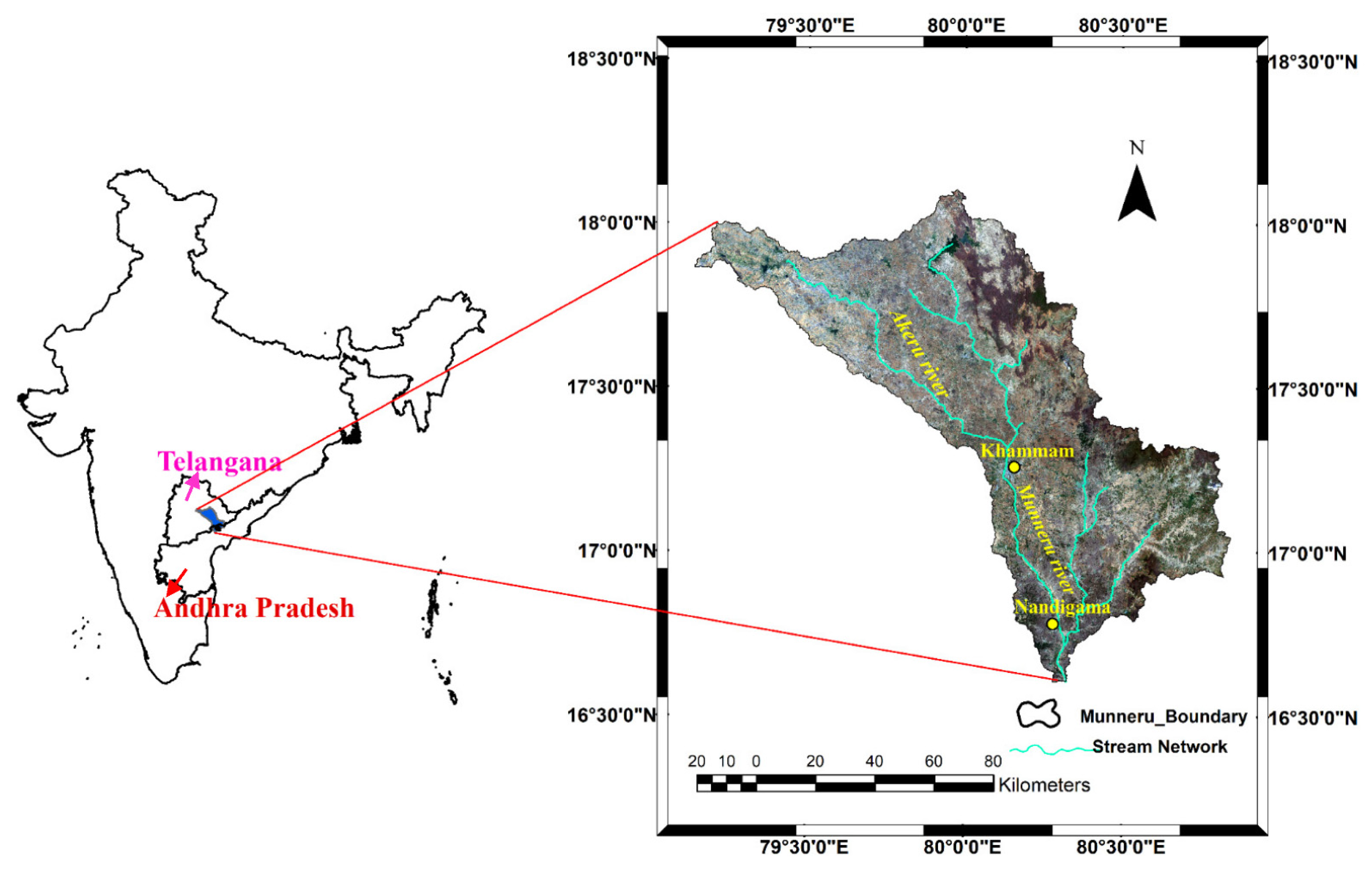
2. Study Area
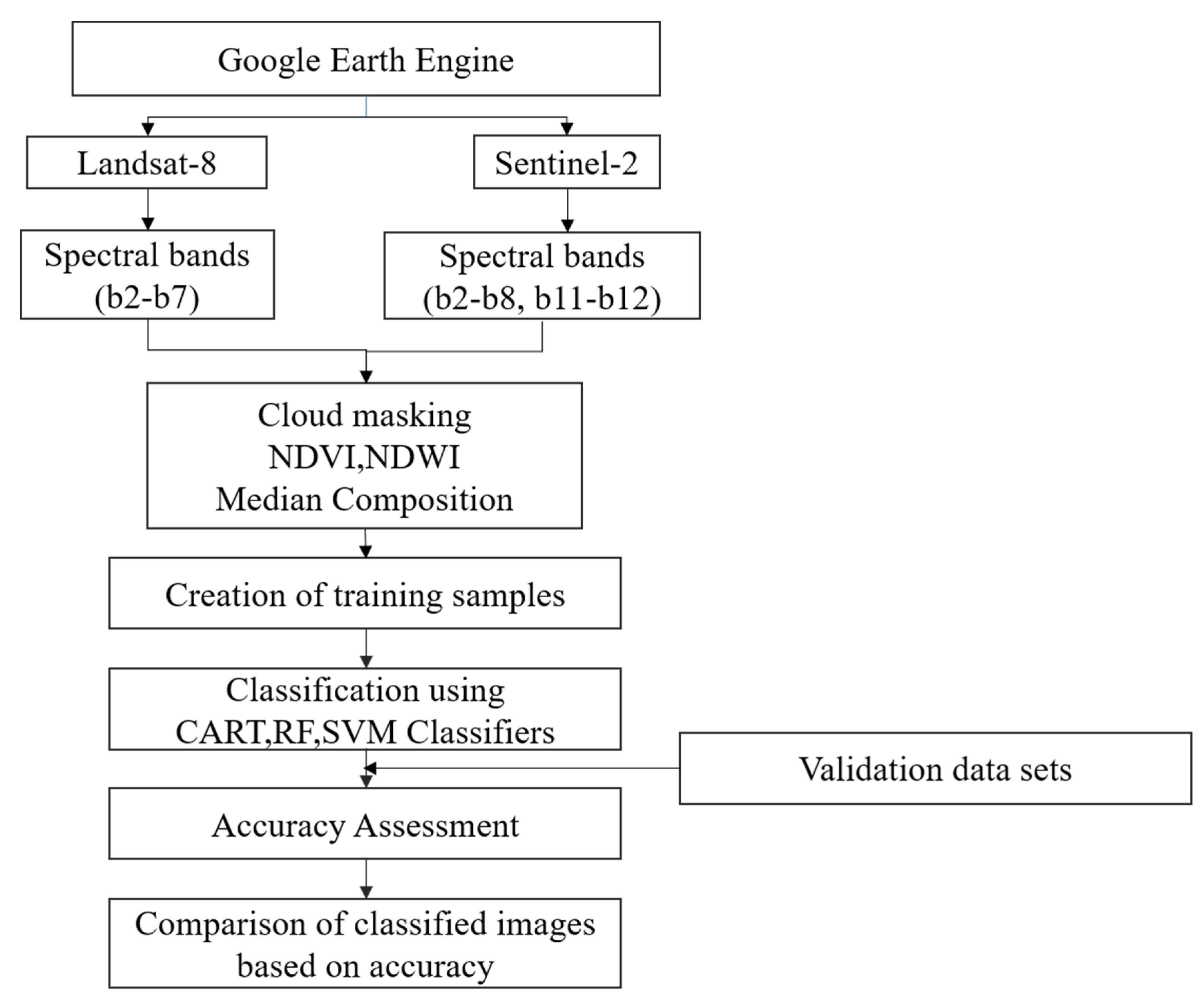
3. Data and Methods
3.1. Data
3.2. Methods
4. Results and Discussion
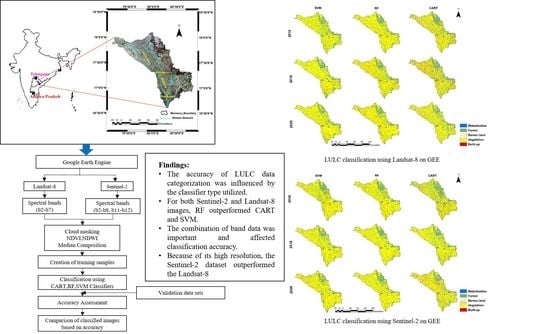
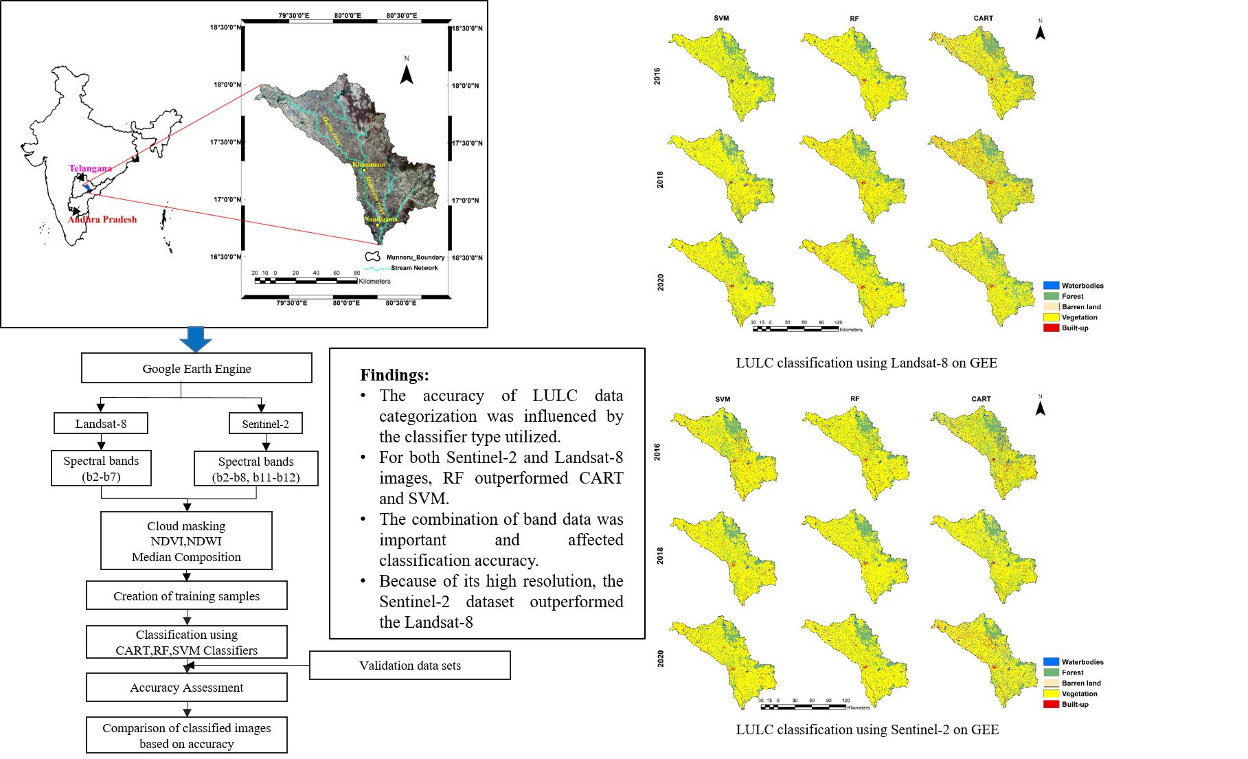
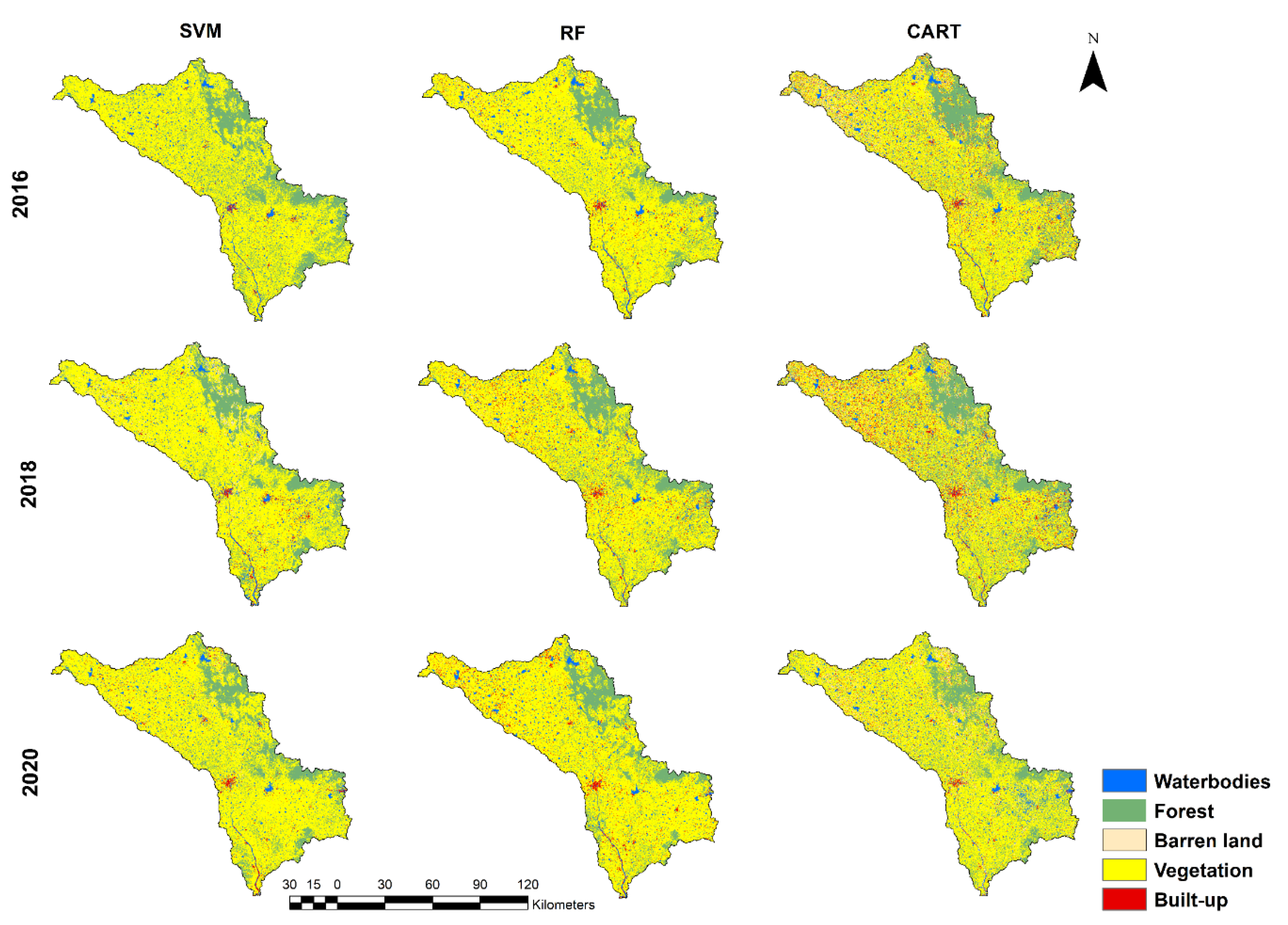
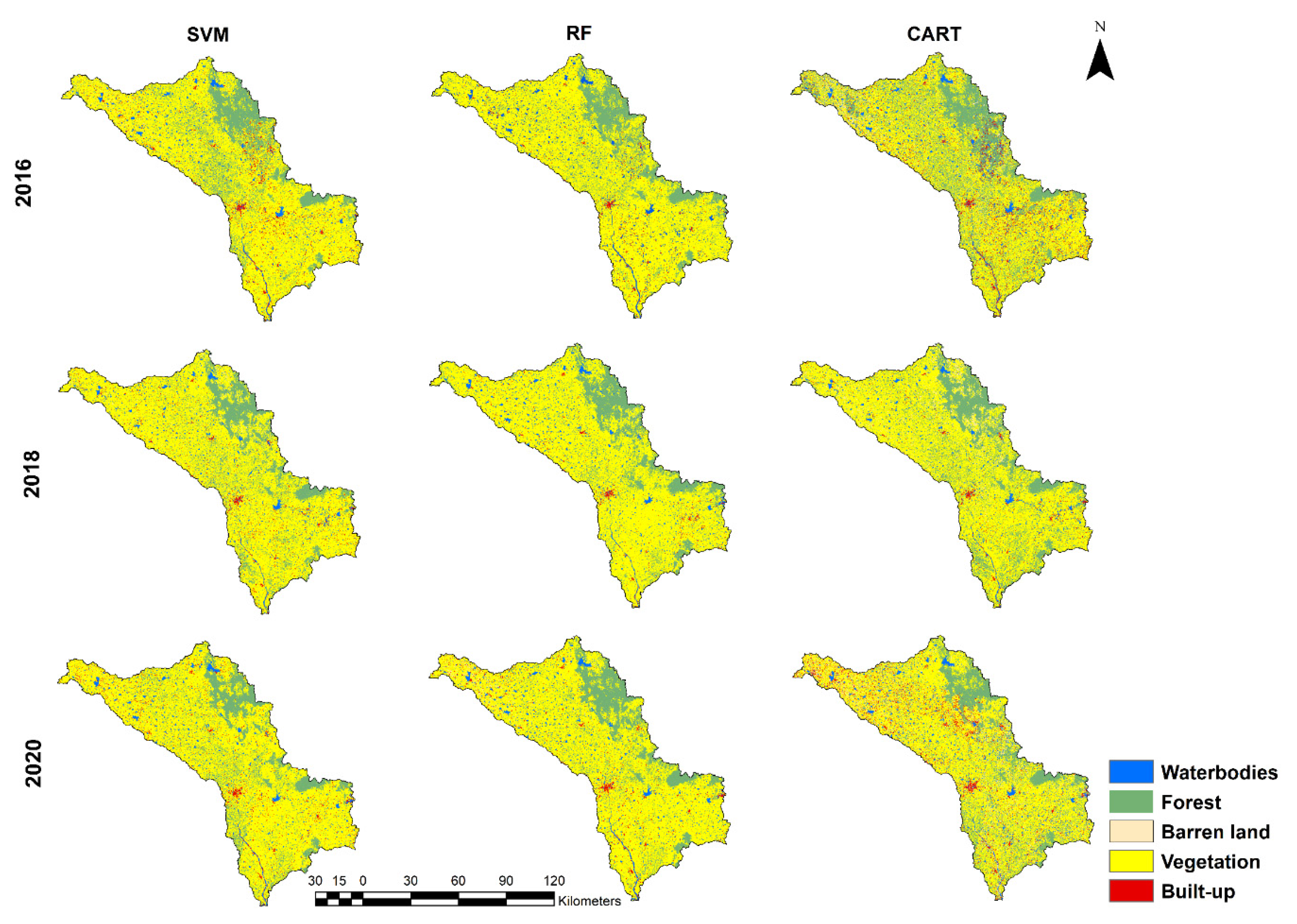
4.1. LULC Classification Using GEE
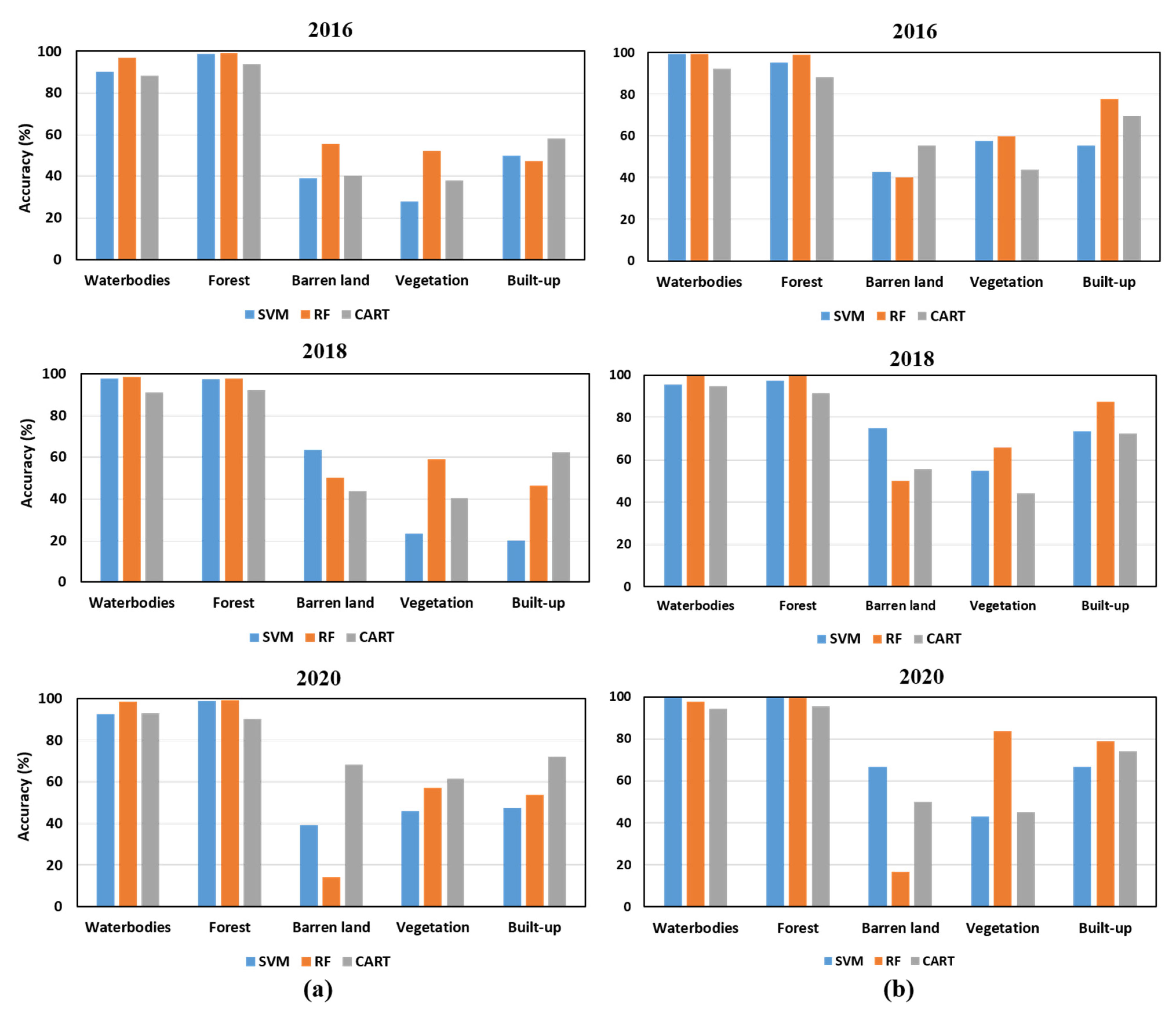
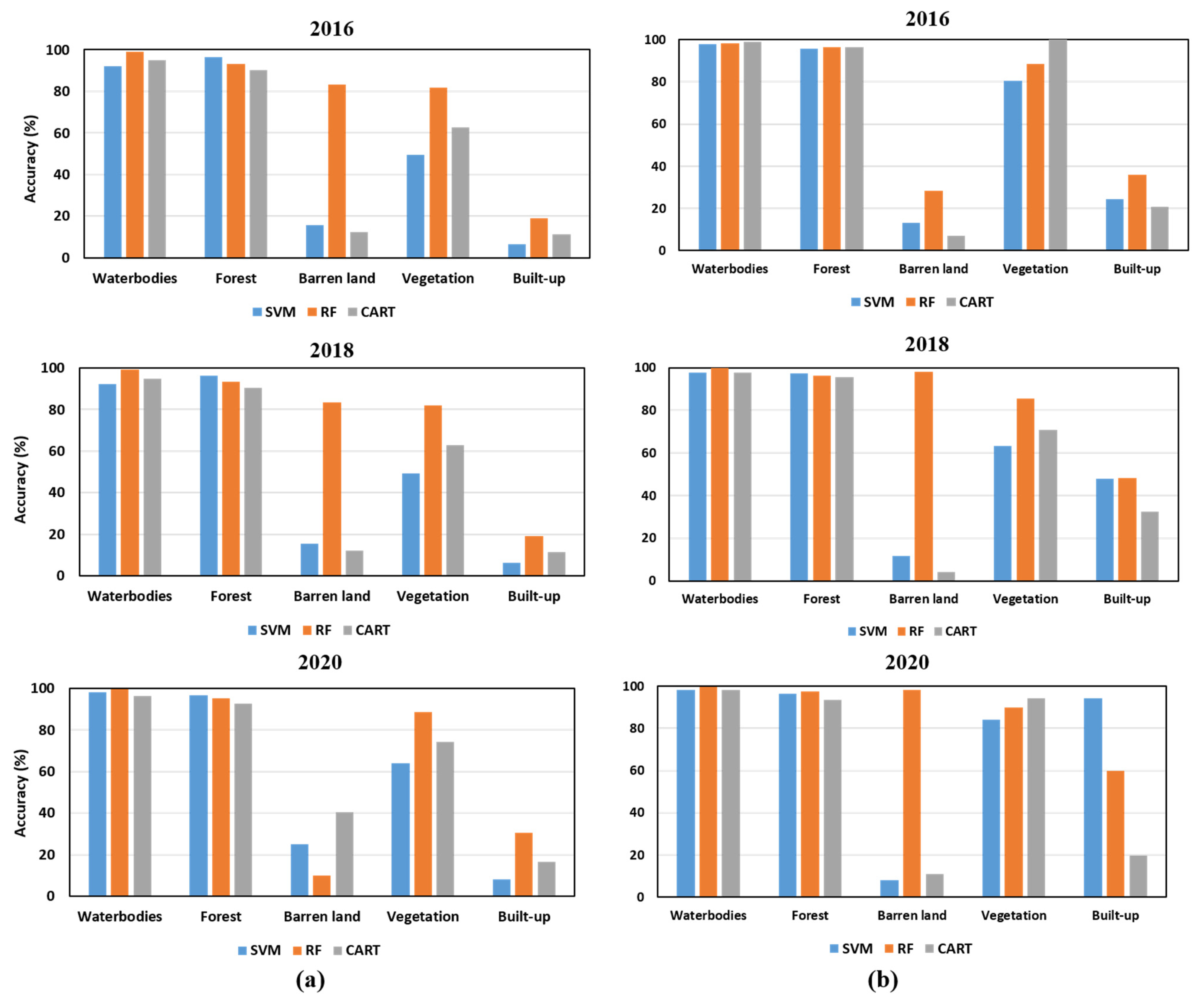
4.2. Comparison of Classification Performances
5. Discussion
6. Conclusions
Author Contributions
Funding
Institutional Review Board Statement
Informed Consent Statement
Data Availability Statement
Conflicts of Interest
References
- Sridhar, V.; Kang, H.; Ali, S.A. Human-Induced Alterations to Land Use and Climate and Their Responses for Hydrology and Water Management in the Mekong River Basin. Water 2019, 11, 1307. [Google Scholar] [CrossRef] [Green Version]
- Sridhar, V.; Jin, X.; Jaksa, W.T.A. Explaining the Hydroclimatic Variability and Change in the Salmon River Basin. Clim. Dyn. 2013, 40, 1921–1937. [Google Scholar] [CrossRef] [Green Version]
- Sujatha, E.R.; Sridhar, V. Spatial Prediction of Erosion Risk of a Small Mountainous Watershed Using RUSLE: A Case-Study of the Palar Sub-Watershed in Kodaikanal, South India. Water 2018, 10, 1608. [Google Scholar] [CrossRef] [Green Version]
- Sridhar, V.; Billah, M.M.; Hildreth, J.W. Coupled Surface and Groundwater Hydrological Modeling in a Changing Climate. Groundwater 2018, 56, 618–635. [Google Scholar] [CrossRef] [PubMed]
- Xiao, Y.; Liu, K.; Yan, H.; Zhou, B.; Huang, X.; Hao, Q.; Zhang, Y.; Zhang, Y.; Liao, X.; Yin, S. Hydrogeochemical Constraints on Groundwater Resource Sustainable Development in the Arid Golmud Alluvial Fan Plain on Tibetan Plateau. Environ. Earth Sci. 2021, 80, 1–17. [Google Scholar] [CrossRef]
- Xiao, Y.; Xiao, D.; Hao, Q.; Liu, K.; Wang, R.; Huang, X.; Liao, X.; Zhang, Y. Accessible Phreatic Groundwater Resources in the Central Shijiazhuang of North China Plain: Perspective From the Hydrogeochemical Constraints. Front. Environ. Sci. 2021, 9, 475. [Google Scholar] [CrossRef]
- Xiao, Y.; Hao, Q.; Zhang, Y.; Zhu, Y.; Yin, S.; Qin, L.; Li, X. Investigating Sources, Driving Forces and Potential Health Risks of Nitrate and Fluoride in Groundwater of a Typical Alluvial Fan Plain. Sci. Total Environ. 2022, 802, 149909. [Google Scholar] [CrossRef]
- Sridhar, V.; Ali, S.A.; Sample, D.J. Systems Analysis of Coupled Natural and Human Processes in the Mekong River Basin. Hydrology 2021, 8, 140. [Google Scholar] [CrossRef]
- Jamali, B.; Bach, P.M.; Cunningham, L.; Deletic, A. A Cellular Automata Fast Flood Evaluation (CA-Ffé) Model. Water Resour. Res. 2019, 55, 4936–4953. [Google Scholar] [CrossRef] [Green Version]
- Rahman, A.; Abdullah, H.M.; Tanzir, M.T.; Hossain, M.J.; Khan, B.M.; Miah, M.G.; Islam, I. Performance of Different Machine Learning Algorithms on Satellite Image Classification in Rural and Urban Setup. Remote Sens. Appl. Soc. Environ. 2020, 20, 100410. [Google Scholar] [CrossRef]
- Sridhar, V.; Anderson, K.A. Human-Induced Modifications to Land Surface Fluxes and Their Implications on Water Management under Past and Future Climate Change Conditions. Agric. For. Meteorol. 2017, 234–235, 66–79. [Google Scholar] [CrossRef] [Green Version]
- Cihlar, J. Land Cover Mapping of Large Areas from Satellites: Status and Research Priorities. Int. J. Remote Sens. 2000, 21, 1093–1114. [Google Scholar] [CrossRef]
- Renschler, C.S.; Harbor, J. Soil Erosion Assessment Tools from Point to Regional Scales—The Role of Geomorphologists in Land Management Research and Implementation. Geomorphology 2002, 47, 189–209. [Google Scholar] [CrossRef]
- Roy, D.P.; Wulder, M.A.; Loveland, T.R.; Woodcock, C.E.; Allen, R.G.; Anderson, M.C.; Helder, D.; Irons, J.R.; Johnson, D.M.; Kennedy, R.; et al. Landsat-8: Science and Product Vision for Terrestrial Global Change Research. Remote Sens. Environ. 2014, 145, 154–172. [Google Scholar] [CrossRef] [Green Version]
- Wulder, M.A.; White, J.C.; Loveland, T.R.; Woodcock, C.E.; Belward, A.S.; Cohen, W.B.; Fosnight, E.A.; Shaw, J.; Masek, J.G.; Roy, D.P. The Global Landsat Archive: Status, Consolidation, and Direction. Remote Sens. Environ. 2016, 185, 271–283. [Google Scholar] [CrossRef] [Green Version]
- Gómez, C.; White, J.C.; Wulder, M.A. Optical Remotely Sensed Time Series Data for Land Cover Classification: A Review. ISPRS J. Photogramm. Remote Sens. 2016, 116, 55–72. [Google Scholar] [CrossRef] [Green Version]
- Noi Phan, T.; Kuch, V.; Lehnert, L.W. Land Cover Classification Using Google Earth Engine and Random Forest Classifier-the Role of Image Composition. Remote Sens. 2020, 12, 2411. [Google Scholar] [CrossRef]
- Sridhar, V.; Hubbard, K.G.; Wedin, D.A. Assessment of soil moisture dynamics of the Nebraska Sandhills using Long-Term measurements and a hydrology model. ASCE J. Irrig. Drain. Engg 2006, 132, 463–473. [Google Scholar] [CrossRef] [Green Version]
- Sridhar, V.; Wedin, D.A. Hydrological behaviour of grasslands of the Sandhills of Nebraska: Water and energy-balance assessment from measurements, treatments, and modelling. Ecohydrol. Ecosyst. Land Water Process Interact. Ecohydrogeomorphol. 2009, 2, 195–212. [Google Scholar] [CrossRef]
- Kang, H.; Sridhar, V.; Mills, B.F.; Hession, W.C.; Ogejo, J.A. Economy-Wide Climate Change Impacts on Green Water Droughts Based on the Hydrologic Simulations. Agric. Syst. 2019, 171, 76–88. [Google Scholar] [CrossRef]
- Setti, S.; Maheswaran, R.; Radha, D.; Sridhar, V.; Barik, K.K.; Narasimham, M.L. Attribution of Hydrologic Changes in a Tropical River Basin to Rainfall Variability and Land-Use Change: Case Study from India. J. Hydrol. Eng. 2020, 25, 05020015. [Google Scholar] [CrossRef]
- Xie, S.; Liu, L.; Zhang, X.; Yang, J.; Chen, X.; Gao, Y. Automatic Land-Cover Mapping Using Landsat Time-Series Data Based on Google Earth Engine. Remote Sens. 2019, 11, 23. [Google Scholar] [CrossRef] [Green Version]
- Gorelick, N.; Hancher, M.; Dixon, M.; Ilyushchenko, S.; Thau, D.; Moore, R. Google Earth Engine: Planetary-Scale Geospatial Analysis for Everyone. Remote Sens. Environ. 2017, 202, 18–27. [Google Scholar] [CrossRef]
- Sidhu, N.; Pebesma, E.; Câmara, G. Using Google Earth Engine to Detect Land Cover Change: Singapore as a Use Case. Eur. J. Remote Sens. 2018, 51, 486–500. [Google Scholar] [CrossRef]
- Tamiminia, H.; Salehi, B.; Mahdianpari, M.; Quackenbush, L.; Adeli, S.; Brisco, B. Google Earth Engine for Geo-Big Data Applications: A Meta-Analysis and Systematic Review. ISPRS J. Photogramm. Remote Sens. 2020, 164, 152–170. [Google Scholar] [CrossRef]
- Kolli, M.K.; Opp, C.; Karthe, D.; Groll, M. Mapping of Major Land-Use Changes in the Kolleru Lake Freshwater Ecosystem by Using Landsat Satellite Images in Google Earth Engine. Water 2020, 12, 2493. [Google Scholar] [CrossRef]
- Shelestov, A.; Lavreniuk, M.; Kussul, N.; Novikov, A.; Skakun, S. Exploring Google Earth Engine Platform for Big Data Processing: Classification of Multi-Temporal Satellite Imagery for Crop Mapping. Front. Earth Sci. 2017, 5, 17. [Google Scholar] [CrossRef] [Green Version]
- Patela, N.N.; Angiuli, E.; Gamba, P.; Gaughan, A.; Lisini, G.; Stevens, F.R.; Tatem, A.J.; Trianni, G. Multitemporal Settlement and Population Mapping from Landsatusing Google Earth Engine. Int. J. Appl. Earth Obs. Geoinf. 2015, 35, 199–208. [Google Scholar] [CrossRef] [Green Version]
- Mateo-García, G.; Gómez-Chova, L.; Amorós-López, J.; Muñoz-Marí, J.; Camps-Valls, G. Multitemporal Cloud Masking in the Google Earth Engine. Remote Sens. 2018, 10, 1079. [Google Scholar] [CrossRef] [Green Version]
- Pimple, U.; Simonetti, D.; Sitthi, A.; Pungkul, S.; Leadprathom, K.; Skupek, H.; Som-ard, J.; Gond, V.; Towprayoon, S. Google Earth Engine Based Three Decadal Landsat Imagery Analysis for Mapping of Mangrove Forests and Its Surroundings in the Trat Province of Thailand. J. Comput. Commun. 2018, 6, 247–264. [Google Scholar] [CrossRef] [Green Version]
- Nery, T.; Sadler, R.; Solis-Aulestia, M.; White, B.; Polyakov, M.; Chalak, M. Comparing Supervised Algorithms in Land Use and Land Cover Classification of a Landsat Time-Series. In Proceedings of the 2016 IEEE International Geoscience and Remote Sensing Symposium (IGARSS), Beijing, China, 10–15 July 2016; pp. 5165–5168. [Google Scholar] [CrossRef]
- Bar, S.; Parida, B.R.; Pandey, A.C. Landsat-8 and Sentinel-2 Based Forest Fire Burn Area Mapping Using Machine Learning Algorithms on GEE Cloud Platform over Uttarakhand, Western Himalaya. Remote Sens. Appl. Soc. Environ. 2020, 18, 100324. [Google Scholar] [CrossRef]
- Liu, D.; Chen, N.; Zhang, X.; Wang, C.; Du, W. Annual Large-Scale Urban Land Mapping Based on Landsat Time Series in Google Earth Engine and OpenStreetMap Data: A Case Study in the Middle Yangtze River Basin. ISPRS J. Photogramm. Remote Sens. 2020, 159, 337–351. [Google Scholar] [CrossRef]
- Tassi, A.; Vizzari, M. Object-Oriented LULC Classification in Google Earth Learning Algorithms. Remote Sens. 2020, 12, 3776. [Google Scholar] [CrossRef]
- Gong, P.; Wang, J.; Yu, L.; Zhao, Y.; Zhao, Y.; Liang, L.; Niu, Z.; Huang, X.; Fu, H.; Liu, S.; et al. Finer resolution observation and monitoring of global land cover: First mapping results with Landsat TM and ETM+ data. Int. J. Remote Sens. 2013, 34, 2607–2654. [Google Scholar] [CrossRef] [Green Version]
- Midekisa, A.; Holl, F.; Savory, D.J.; Andrade-Pacheco, R.; Gething, P.W.; Bennett, A.; Sturrock, H.J.W. Mapping land cover change over continental Africa using Landsat and Google Earth Engine cloud computing. PLoS ONE 2017, 12, e0184926. [Google Scholar] [CrossRef]
- Dong, J.; Xiao, X.; Menarguez, M.A.; Zhang, G.; Qin, Y.; Thau, D.; Biradar, C.; Moore, B. Mapping Paddy Rice Planting Area in Northeastern Asia with Landsat 8 Images, Phenology-Based Algorithm and Google Earth Engine. Remote Sens. Environ. 2016, 185, 142–154. [Google Scholar] [CrossRef] [Green Version]
- Aguilar, R.; Zurita-Milla, R.; Izquierdo-Verdiguier, E.; de By, R.A. A Cloud-Based Multi-Temporal Ensemble Classifier to Map Smallholder Farming Systems. Remote Sens. 2018, 10, 729. [Google Scholar] [CrossRef] [Green Version]
- Workie, T.G.; Debella, H.J. Climate Change and Its Effects on Vegetation Phenology across Ecoregions of Ethiopia. Glob. Ecol. Conserv. 2018, 13, e00366. [Google Scholar] [CrossRef]
- Jamei, Y.; Rajagopalan, P.; Sun, Q.C. Time-Series Dataset on Land Surface Temperature, Vegetation, Built up Areas and Other Climatic Factors in Top 20 Global Cities (2000–2018). Data Br. 2019, 23, 103803. [Google Scholar] [CrossRef]
- Wang, C.; Jia, M.; Chen, N.; Wang, W. Long-Term Surface Water Dynamics Analysis Based on Landsat Imagery and the Google Earth Engine Platform: A Case Study in the Middle Yangtze River Basin. Remote Sens. 2018, 10, 1635. [Google Scholar] [CrossRef] [Green Version]
- Simonetti, D.; Simonetti, E.; Szantoi, Z.; Lupi, A.; Eva, H.D. First Results from the Phenology-Based Synthesis Classifier Using Landsat 8 Imagery. IEEE Geosci. Remote Sens. Lett. 2015, 12, 1496–1500. [Google Scholar] [CrossRef]
- Zurqani, H.A.; Post, C.J.; Mikhailova, E.A.; Schlautman, M.A.; Sharp, J.L. Geospatial Analysis of Land Use Change in the Savannah River Basin Using Google Earth Engine. Int. J. Appl. Earth Obs. Geoinf. 2018, 69, 175–185. [Google Scholar] [CrossRef]
- Tucker, C.J. Red and Photographic Infrared Linear Combinations for Monitoring Vegetation. Remote Sens. Environ. 1979, 8, 127–150. [Google Scholar] [CrossRef] [Green Version]
- McFeeters, S.K. The Use of the Normalized Difference Water Index (NDWI) in the Delineation of Open Water Features. Int. J. Remote Sens. 1996, 17, 1425–1432. [Google Scholar] [CrossRef]
- Brieman, L.; Friedman, J.H.; Olshen, R.A.; Stone, C.J. Classification and Regression Trees, 1st ed.; Routledge: London, UK, 1984; Volume 45, pp. 5–32. [Google Scholar] [CrossRef]
- Breiman, L. Random Forests. Mach. Learn. 2001, 45, 5–32. [Google Scholar] [CrossRef] [Green Version]
- Belgiu, M.; Drăgu, L. Random Forest in Remote Sensing: A Review of Applications and Future Directions. ISPRS J. Photogramm. Remote Sens. 2016, 114, 24–31. [Google Scholar] [CrossRef]
- Hsu, C.W.; Chang, C.C.; Lin, C.J. A Practical Guide to Support Vector Classification; Technical Report; Department of Computer Science and Information Engineering, University of National Taiwan: Taipei, Taiwan, 2003; pp. 1–12. Available online: https://www.csie.ntu.edu.tw/~cjlin/papers/guide/guide.pdf (accessed on 8 December 2021).
- Thomas, L.; Ralph, W.; Kiefer, J.C. Remote Sensing and Image Interpretation (Fifth Edition). Geogr. J. 2004, 146, 448–449. [Google Scholar]
- Kohavi, R. A Study of Cross-Validation and Bootstrap for Accuracy Estimation and Model Selection. Int. Jt. Conf. Artif. Intell. 1995, 14, 1137–1145. [Google Scholar]
- Stehman, S.V. Sampling Designs for Accuracy Assessment of Land Cover. Int. J. Remote Sens. 2009, 30, 5243–5272. [Google Scholar] [CrossRef]
- Pal, M.; Foody, G.M. Evaluation of SVM, RVM and SMLR for Accurate Image Classification with Limited Ground Data. IEEE J. Sel. Top. Appl. Earth Obs. Remote Sens. 2012, 5, 1344–1355. [Google Scholar] [CrossRef]
- Shetty, S. Analysis of Machine Learning Classifiers for LULC Classification on Google Earth Engine Analysis of Machine Learning Classifiers for LULC Classification on Google Earth Engine. Master’s thesis, University of Twente, Enschede, The Netherlands, 2019; pp. 1–65. [Google Scholar]
- Chang, K.T.; Merghadi, A.; Yunus, A.P.; Pham, B.T.; Dou, J. Evaluating Scale Effects of Topographic Variables in Landslide Susceptibility Models Using GIS-Based Machine Learning Techniques. Sci. Rep. 2019, 9, 12296. [Google Scholar] [CrossRef] [PubMed] [Green Version]
- Shao, Y.; Lunetta, R.S. Comparison of Support Vector Machine, Neural Network, and CART Algorithms for the Land-Cover Classification Using Limited Training Data Points. ISPRS J. Photogramm. Remote Sens. 2012, 70, 78–87. [Google Scholar] [CrossRef]
- Goldblatt, R.; You, W.; Hanson, G.; Khandelwal, A.K. Detecting the Boundaries of Urban Areas in India: A Dataset for Pixel-Based Image Classification in Google Earth Engine. Remote Sens. 2016, 8, 634. [Google Scholar] [CrossRef] [Green Version]
- Congalton, R.G.; Green, K. Assessing the Accuracy of Remotely Sensed Data: Principles and Practices, 3rd ed.; CRC Press: Boca Raton, FL, USA, 2019. [Google Scholar] [CrossRef]


| Data Layer | Source | Bands Used | Central Wavelength (µm) | Band Width (µm) | Spatial Resolution (m) |
|---|---|---|---|---|---|
| Landsat-8 Operational Land Imager surface reflectance Tier 1 | Google Earth Engine (GEE), data accessed via the U.S. Geological Survey (USGS) | Blue (Band 2) | 0.482 | 0.060 | 30 |
| Green (Band 3) | 0.561 | 0.057 | 30 | ||
| Red (Band 4) | 0.655 | 0.038 | 30 | ||
| Near-Infra-Red (Band 5) | 0.865 | 0.028 | 30 | ||
| Short-Wave Infra-Red 1 (Band 6) | 1.609 | 0.085 | 30 | ||
| Short-Wave Infra-Red 2 (Band 7) | 2.200 | 0.186 | 30 | ||
| Sentinel-2 MSI: MultiSpectral Instrument, Level-1C | Google Earth Engine (GEE), data accessed via the U.S. Geological Survey (USGS) | Blue (Band 2) | 0.496 | 0.066 | 10 |
| Green (Band 3) | 0.560 | 0.036 | 10 | ||
| Red (Band 4) | 0.664 | 0.031 | 10 | ||
| Red-Edge 1(Band 5) | 0.704 | 0.015 | 20 | ||
| Red-Edge 2 (Band 6) | 0.740 | 0.015 | 20 | ||
| Red-Edge 3 (Band 7) | 0.782 | 0.020 | 20 | ||
| Near-Infra-Red (Band 8) | 0.835 | 0.106 | 10 | ||
| Short-Wave Infra-Red 1 (Band 11) | 1.610 | 0.091 | 20 | ||
| Short-Wave Infra-Red 2 (Band 12) | 2.202 | 0.175 | 20 |
| Year | Classifier | Landsat-8 | Sentinel-2 | ||
|---|---|---|---|---|---|
| Overall Accuracy (%) | Kappa Coefficient | Overall Accuracy (%) | Kappa Coefficient | ||
| 2016 | SVM | 88.99 | 0.81 | 92.37 | 0.868 |
| RF | 93.93 | 0.89 | 94.65 | 0.904 | |
| CART | 81.61 | 0.72 | 84.75 | 0.747 | |
| 2018 | SVM | 91.62 | 0.85 | 93.05 | 0.878 |
| RF | 94.86 | 0.91 | 95.85 | 0.928 | |
| CART | 82.59 | 0.73 | 85.88 | 0.772 | |
| 2020 | SVM | 92.95 | 0.87 | 95.54 | 0.918 |
| RF | 95.84 | 0.92 | 97.04 | 0.947 | |
| CART | 86.58 | 0.79 | 88.81 | 0.814 | |
Publisher’s Note: MDPI stays neutral with regard to jurisdictional claims in published maps and institutional affiliations. |
© 2021 by the authors. Licensee MDPI, Basel, Switzerland. This article is an open access article distributed under the terms and conditions of the Creative Commons Attribution (CC BY) license (https://creativecommons.org/licenses/by/4.0/).
Share and Cite
Loukika, K.N.; Keesara, V.R.; Sridhar, V. Analysis of Land Use and Land Cover Using Machine Learning Algorithms on Google Earth Engine for Munneru River Basin, India. Sustainability 2021, 13, 13758. https://doi.org/10.3390/su132413758
Loukika KN, Keesara VR, Sridhar V. Analysis of Land Use and Land Cover Using Machine Learning Algorithms on Google Earth Engine for Munneru River Basin, India. Sustainability. 2021; 13(24):13758. https://doi.org/10.3390/su132413758
Chicago/Turabian StyleLoukika, Kotapati Narayana, Venkata Reddy Keesara, and Venkataramana Sridhar. 2021. "Analysis of Land Use and Land Cover Using Machine Learning Algorithms on Google Earth Engine for Munneru River Basin, India" Sustainability 13, no. 24: 13758. https://doi.org/10.3390/su132413758
APA StyleLoukika, K. N., Keesara, V. R., & Sridhar, V. (2021). Analysis of Land Use and Land Cover Using Machine Learning Algorithms on Google Earth Engine for Munneru River Basin, India. Sustainability, 13(24), 13758. https://doi.org/10.3390/su132413758