
Static and Seismic Responses of Eco-Friendly Buried Concrete Pipes with Various Dosages of Fly Ash


School of Engineering, University of Greenwich, Kent ME4 4TB, UK
*
Author to whom correspondence should be addressed.
Appl. Sci. 2021, 11(24), 11700; https://doi.org/10.3390/app112411700
Submission received: 19 September 2021
/
Revised: 23 November 2021
/
Accepted: 24 November 2021
/
Published: 9 December 2021
(This article belongs to the Special Issue Seismic Vulnerability Assessment for Civil and Industrial Infrastructures)
Abstract
:In this paper, an evaluation based on the detailed failure has been conducted for underground sewage Geopolymer concrete (GPC) pipes under static and seismic loadings with consideration of the optimal time steps in the time-dependent process related to nonlinear behavior of GPC pipes in static and dynamic analyses. The ANSYS platform is employed for improving an advanced FE model for a GPC pipe which can simulate the performance of underground GPC pipes containing various percentages of fly ash (FA) as a Portland cement (PC) replacement. Subsequently, the time-dependent model is used to assess the efficacy of this concrete admixture (FA) in the structural response of the unreinforced GPC pipe in FEM. Indeed, the generated GPC pipe with the three-dimensional model has the potential to capture the nonlinear behavior of concrete which depicts the patterns of tensile cracking and compressive crushing that occur over the applied static loads in the FE model. The main issue in this paper is the assessment of the GPC pipe response typically based on the displacement due to static and seismic loadings. The numerical results demonstrated that the optimal displacement was obtained when the structural response had typically the lowest value for GPC pipes containing 10–30% FA and 20% FA under static and seismic loadings, respectively. Indeed, a reduction by 25% for the vertical displacement of a GPC pipe containing 20% FA was observed compared to that without FA under time-history analysis.
1. Introduction
The issue of an appropriate collapse probability along with the optimal response of underground concrete pipes has been highlighted in numerous investigations. Indeed, the reduction of vertical and horizontal displacement as the optimal response of buried GPC pipes under static and seismic loading is the central challenge for evaluating the structural performance of underground GPC pipes which need to be improved through reorganizing the effects of material properties of GPC and other main factors on the structural performance of GPC pipes. Based on preliminary studies, the mechanical properties of concrete (compressive strength, flexural strength) and FA inclusion in concrete content are two significant factors in the behavioral performance of concrete elements such as concrete cubes and beams [1,2,3,4,5,6,7].
Numerous investigations on the performance and design of underground pipes have been carried out using either static or dynamic loads without any precise vindication related to the section of loading type [8,9,10]. Chaallal et al. [11] investigated the behavior of underground flexible pipes under static loading. Moreover, Rakitin and Xu [12], MacDougall et al. [13], and Lay and Brachman [14] explored the behavior and the design of underground concrete pipes under static surface loads. On the other hand, McGrath et al. [15] presented the results of an investigation on the response of a buried flexible pipe for moving truckloads under the maximum load of 107 kN. Li et al. [16] reported the response of a buried concrete pipe and a rectangular culvert under the effect of a moving aircraft wheel load by FEM. Eventually, Neya et al. [17] conducted a three-dimensional FE study on the behavior of a buried pressurized steel pipe. Other research activities were also conducted using a 3D FE analysis, such as [8,11,12,13,14,15,16,17,18].
In summary, it cannot be conclusively approved by previous investigations whether a static or a dynamic load needs to be applied to assess the behavior of underground pipes. Thus, this study aims to acquire the critical loading conditions on GPC pipes, hence, the major contributions of this study are presented as follows:
- ➢
- A robust 3D finite element model is developed for evaluating the optimal displacement of GPC pipes by utilizing fault displacement (static loading) and records of the actual earthquake (seismic loading) as well as traffic loads and self-weight of soil and GPC pipe as live and dead loads in this study;
- ➢
- The possibility of relative comparison of seismic and static responses of buried pipes under the influence of GPC properties is developed in this field;
- ➢
- The utilization of element types of solid 185 and pipe 288 compatible with the proposed nonlinear model such as Drucker–Prager has been applied for the first time in this study after validating with similar element types such as solid 65 used in previous investigations.
2. Finite Element Modeling
2.1. Determination of Basic Equations for the Stress–Strain Curve of GPC
After reviewing the variety of constitutive models for GPC in compression state, Table 1 represents the six most widely accepted models which are relatively compatible for GPC in low-calcium classification (class F). The linear state of stress–strain relations in the ascending branch was kept unchanged for all these six models. However, the curvatures of the stress–strain relations after peak stress in the descending branch have a distinctive difference which varies by replacing diverse values for the parameter ‘n’ in the empirical formula experimentally obtained in previous investigations. As shown in Figure 1, ‘n’ is attributed to the peak stress value. Additionally, Fan et al. [19] demonstrated that the parameter ‘n’ at different temperatures can play an effective role in the nonlinear behavior of concrete in the descending region at the collapse moment. It was proved that ‘n’ has a significant effect on the nonlinear behavior of concrete resulting in less plastic strain in the concrete specimens containing FA compared to those with conventional paste such as OPC. This occurrence can be ascribed due to the increase of the CSH chain caused by a chemical reaction between FA and PC. The increase of ‘n’ that rapidly occurred at an early stage is due to amplification of the reaction at temperatures between 9–200 °C as shown in Figure 1. On the contrary, the decrement of ‘n’ at a later stage might be caused by the appearance of the thermally induced microcracks in cement paste and decomposition of the CSH chain. In this study, the value of n = 4 was chosen for the Popovic relation proposed in 1971, given that the curing condition for the experimental schedule of the current study was kept under the temperature of 21 °C (the temperature at water bath).
With respect to Ec as the significant parameter in the stress–strain curve, most early studies, as well as current investigations, centralize on Ec of GPC mixture at 28 days of age. For instance, Nath and Sarkar [20] presented a relationship (Equation (1)) based on their experimental observations to predict the elastic modulus of ambient cured blended low calcium FA-based GPC mixes as follows:
where Ecj.a is the elastic modulus of ambient cured FA-based GPC in MPa. In addition, Waqas et al. [21] have recently explored an empirical formula to predict the elasticity modulus of ambient cured fly ash and slag-based geopolymer concrete (FS-GPC) as given by Equation (2):
where Ec is the elastic modulus of concrete (GPA) and fc is the average compressive strength measured on cubes (MPa). In the current study, the two above-mentioned relations for the value of Ec are selected for the modified Popovics relations proposed by Isojed et al. [22] and Halahla [23] (Table 1). It is essential to mention that only the amounts of strain corresponding to the peak-stress of these two relations are attributed to Ec; whereas other proposed constitutive models are in relation to as shown in Table 1.

Table 1.
Constitutive models for GPC concrete in compression state.
| Proposed Model | Constitutive Models Equation for GPC Concrete | ||
|---|---|---|---|
| Modified Popovics function, (Isojeh et al. [22]) | < 1.0 → k = 1 | [Equation (1)] [Equation (2)] | |
| Modifed Popovics function (Halahla [23]) | |||
| Popovics [24] | N = 0.058 f’c + 1 | N/A | |
| Fan et al. [19] | n = 4 | N/A | |
| Popovics [25] and Mander et al. [26] | |||
| EN 1992-1-1 [27] | N/A |
Validation of the Developed Constitutive Model for GPC Concrete
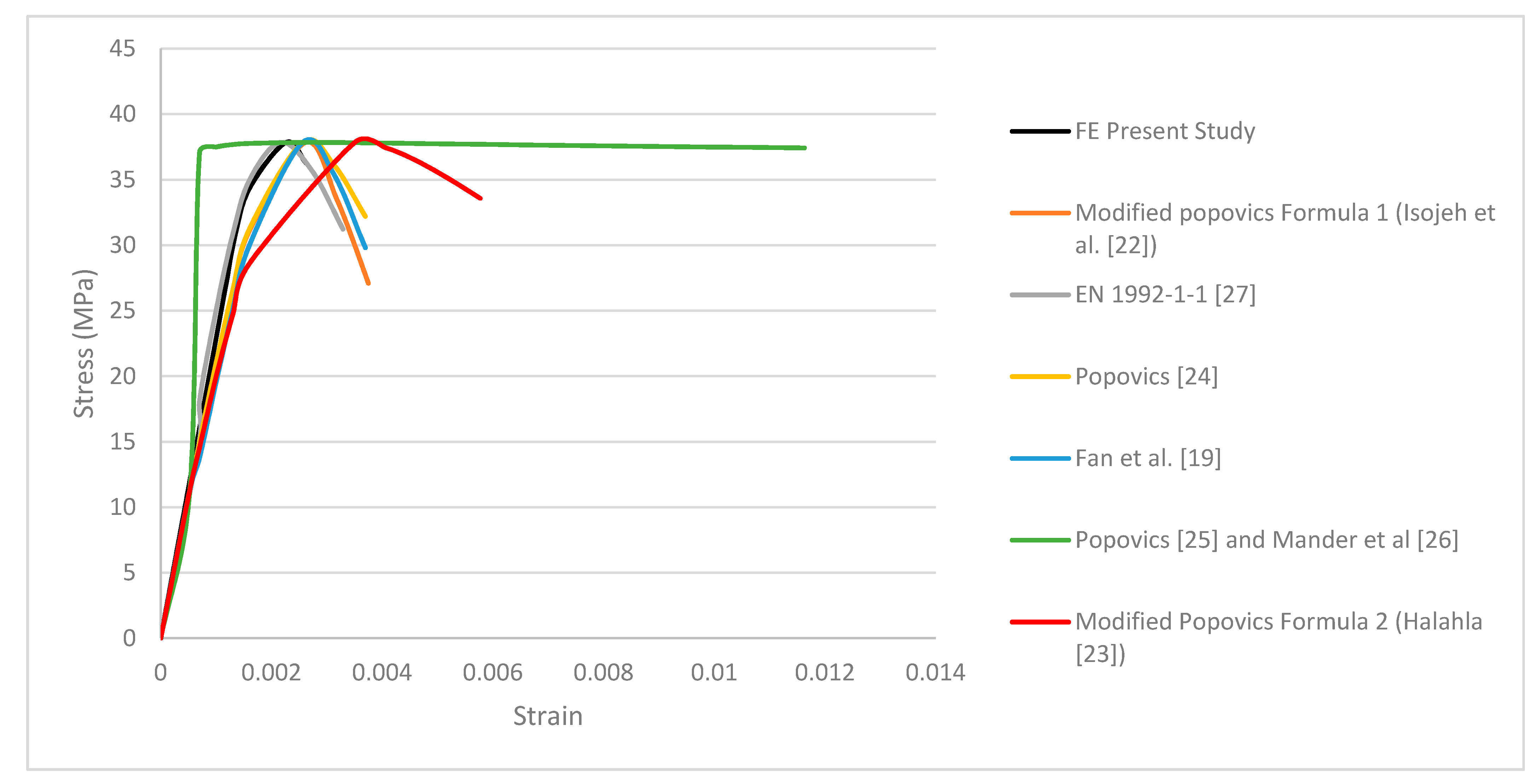
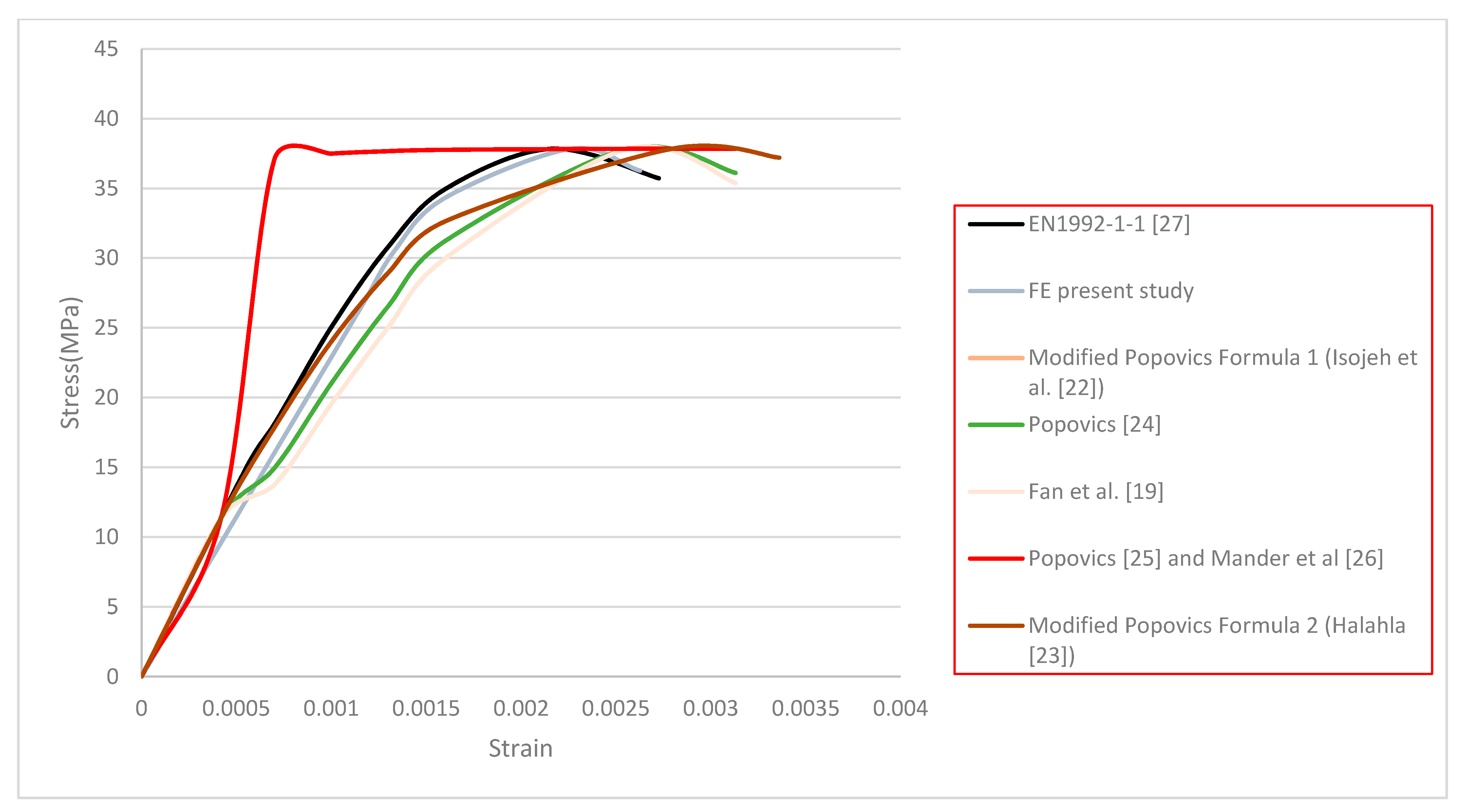
The comparison between stress–strain curves subjected to FE results of the GPC cube in the present study and those relations discussed in Section 2.1 are represented in Figure 2 and Figure 3. It is clear from this comparative assessment that the numerical model of this study behaves excellently with the proposed relations. However, there is a relatively significant difference that can be seen from the relation presented by Popovics [25] and Mander et al. [26] referring to the different values of ‘n’ as explained in Section 2.1. On the other hand, after comparing the stress–strain relationship subjected to FE results of a concrete cube containing 20% FA, numerically obtained in the current study, to other examined constitutive models for compression state of concrete based on Popovics formulations and Eurocode standards, it is proved that the numerical results of the current study have a relatively high approximation with the proposed constitutive models which were found through other empirical functions, especially Eurocode and Popovic relations [22,23,24,25,26,27]. The value of the ‘n’ parameter for the constitutive model presented by Fan et al. [19] in the range of 3–4 is strongly recommended for this concrete type with a low calcium amount. It is necessary to point out that the experimental data achieved in the present study (compressive strength for 20% FA, and concrete density) were utilized for defining material properties in the FE model of GPC.
From Figure 2 and Figure 3, it can be observed that the predictions of constitutive models by Isojeh et al. [22] and EN1992-1-1 [27] are the closest to the numerical results of the present study, while the equations presented by Popovics [25] andMander et al. [26] and Fan et al. [19], Halahla [23] yield lower and higher values, respectively, than the current study. Hence, the developed constitutive concrete model using the modified Popovics model recommended by Isojeh et al. [22] using Equation (2) for calculating Ec was chosen as the basic equation for concrete specimens involving 20% FA content at age of 28 days, to assess the nonlinear (cracking and crushing) behavior of this concrete type for the next stages of this study.
In addition, the William–Warneke failure criterion, involving nine parameters (Table 2) was considered for describing the nonlinear behavior of GPC. Three key parameters play a major role in calibrating the constitutive model. These parameters are ultimate stress, ultimate strain, and the slope of the stress–strain curve for the initial part of the ascending zone of the stress–strain curve. Other parameters associated with the nonlinear behavior of GPC have been selected considering the highest degree of adaption with these three parameters. The ultimate load, stress, and strain predicted by the numerical model are 0.7%, 0.79%, and 8.4% higher than those achieved through the modified Popovics relation (Table 3). Hence, the calibrated model with the concrete properties defined in this numerical simulation can be used for other GPC structures which will be modelled in FE.
2.2. Model Validation
In the next stage, the numerical results are calibrated with those in the study conducted by Zamarian [28] in similar conditions (model dimension, applied load, etc.) as shown in Table 4, Figure 4 and Figure 5. It is worth pointing out that the value of traffic load as the live load is based on the details of the American Association of State Highway and Transportation Officials (AASTHO) standard.
The following constants are desired for defining concrete properties in the ANSYS platform (Table 2):
- -
- Shear transfer coefficients for an open crack (βt);
- -
- Shear transfer coefficients for a closed crack (βc);
- -
- Uniaxial tensile cracking stress (ft);
- -
- Uniaxial crushing stress (positive) (fcu);
- -
- Biaxial crushing stress (positive) (fcb);
- -
- Ambient hydrostatic stress state (σha);
- -
- Biaxial crushing stress (positive) (f1);
- -
- Uniaxial crushing stress (positive) (f2);
- -
- Stiffness multiplier for cracked tensile condition (Tc).
Four parameters, namely the shear transfer coefficients for an open crack (βt), the shear transfer coefficients for a closed crack (βc), the uniaxial tensile cracking stress (ft), and the uniaxial crushing stress (fcu), are more important compared to other concrete properties. The shear transfer coefficients, (βt) and (βc), are used to consider the retention of shear stiffness in cracked concrete; these parameters range from 0 to 1.0, with 0 representing a smooth crack (complete loss of shear transfer) and 1.0 representing a rough crack (no loss of shear transfer) (ANSYS [29]). For this study, the shear transfer coefficient for an open crack (βt) is set to 0.3 to avoid convergence problems and the shear transfer coefficients for a closed crack (βc) is chosen as 1.0 [3,30,31,32,33,34].
Further details related to soil and concrete properties used in this validation are presented in Table 5. It is observed that the element types used in the current study are pipe 188 and solid 185 for concrete and soil, respectively, whereas the element type applied was solid 65 for both concrete and soil in the previous study.
As can be seen in Figure 6, the values of the stress–strain curve have a relatively high approximation, so that the maximum values of stress for both numerical models have a minimum difference of 5%, which means that the numerical model used in this study is reliable.
2.3. Material Properties of Soil and GPC in FE Modeling
After validating the underground concrete pipe model with acceptable satisfaction according to the numerical results presented in Section 2.2, two typical types of soils (backfill, sidefill and bedding) have been used for FE analysis of underground GPC pipes to execute the investigation for detecting the interaction between soil and an underground pipeline. As a result, based on the validation of two different element types (Soild 65, Solid 185) with the excellent agreement for soil conducted in Section 2.2, it can be found that Solid 185 is the element surrounding underground GPC pipes that can withstand against uplift forces with displacements in a reasonable range. This study represents the FE modeling with the use of SOLID 185 for the surrounded soils of GPC pipes to assess the accurate response of the GPC pipe with an optimal displacement under static and seismic loadings. Further details in the case of elastic and plastic properties of the GPC pipe and soil types are exhibited in Table 6. It is worth mentioning that the maximum values corresponding to material properties of two soil types have been applied for the FE model to provide the most critical state while analyzing the GPC pipe model under static and seismic loadings.
2.3.1. Selection of GPC Pipe Size
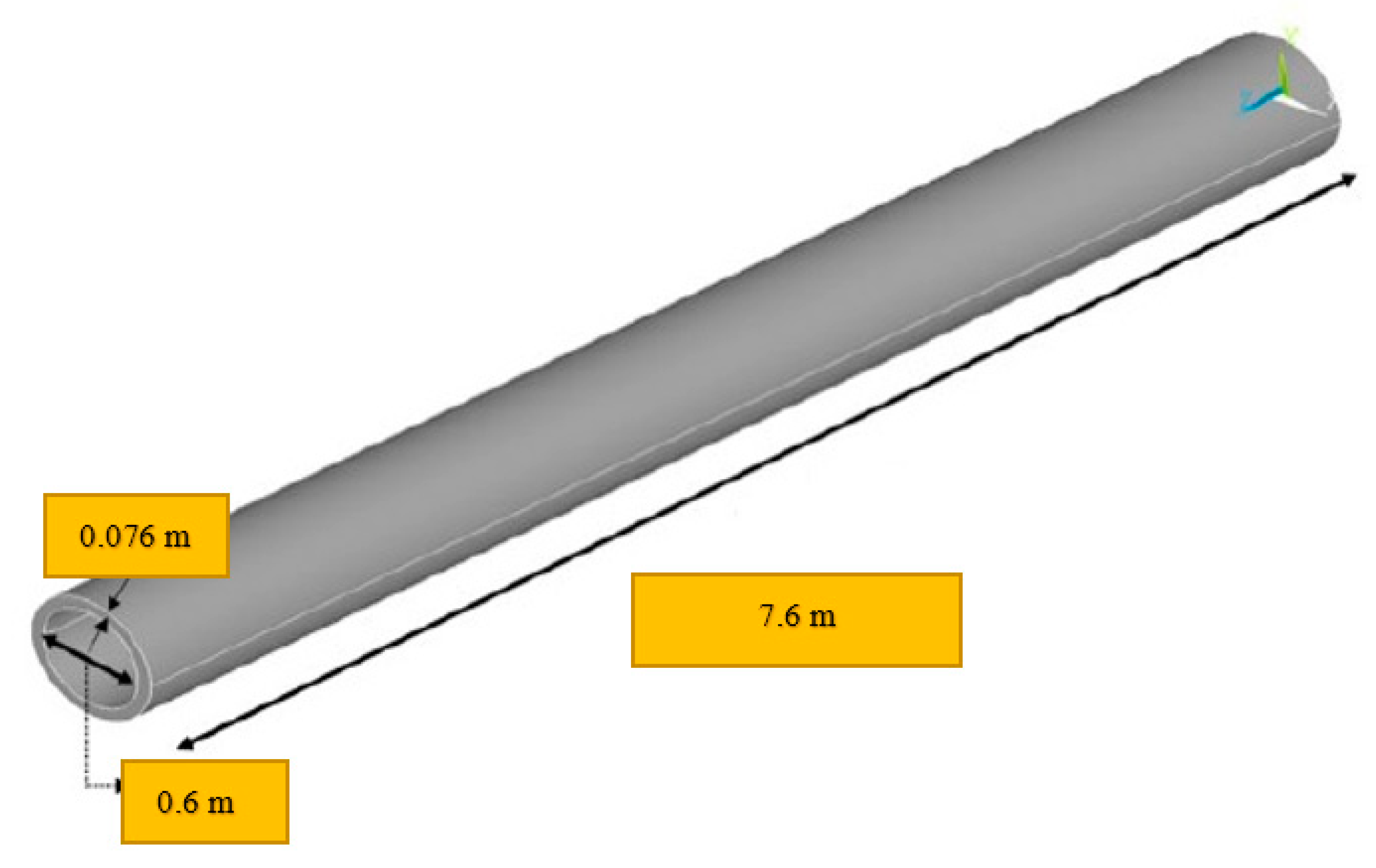
The unreinforced concrete pipe numerically validated in Section 2.2, was chosen as a 3D FE model for a buried GPC pipe in the current study. In addition, the soil geometries need to be defined for this FEM. The dimensions of the GPC pipe are in accordance with ASTM Specification C14–15 based on the American Association of State Highway and Transportation Officials (AASHTO) as shown in Table 7.
It is essential to mention that this pipe type is a Class-II non-reinforced concrete pipe category which is commonly used in the industry. The length of the pipe is chosen to be 10 times of the pipe’s diameter to reduce the effect of boundary conditions on numerical results of the study as shown in Figure 7 [28,35].
For modeling the surrounded soil, the details of standard design considering the suggestion of the American Concrete Pipe Association have been utilized in this study. Therefore, two volumes are each assumed for the bedding—siding and backfill soil. As shown in Figure 4 and Table 8, the minimum bedding thickness (15.24 cm) is used. According to ACPA, the minimum trench width is approximately 1.524 m for a non-reinforced round concrete pipe with 0.762 m outer diameter [28,35].
According to the details of Type 4 soil (Table 8), the minimum width of the sidefill is 18 in. So, the overall width of the trench can be calculated by WT = 2 × (0.4572 m) + Do = 2 × 0.4572 + 0.762 = 1.676 m. Hence, the overall width of the trench (WT) is proposed to be 1.676 m, where Do is the outer diameter.
2.3.2. Selection of Element Type for GPC Pipe
The concrete behavioral model in the ANSYS platform, derived from the William–Varnke model, is used to simulate the nonlinear behavior of concrete in the ANSYS finite element software. This criterion is also utilized to predict the damages that occurred in concrete and other frictional adhesives, such as masonry materials, soil, and rock. The significant point is the fact that the concrete behavioral model in the ANSYS software is to be applied through the three-dimensional geometric model which is the element compatible with the concrete model. That means the elements in 1D or 2D are not suitable for this purpose. So, after the validation of the elements of Pipe 288 and Solid 65 resulted in the excellent agreement, Pipe 288 has been chosen for the first time to simulate the concrete behavior of the buried GPC pipe. The pipeline is simulated with a length of 7.6 m under AASTHO and ASTM standards which is presented in Figure 5. In addition, Figure 8 shows the details of Pipe 288 as the element type used in the FE model of the GPC pipe.
To cast more clarification on the offered points, the significant features related to the performance of Pipe 288 element will be briefly put forward in the following statements:
- ➢
- The mesh size chosen for the pipe 288 is 0.5 m, as it is observed that this value gives better convergence in the nonlinear analysis compared to other mesh sizes examined in the study;
- ➢
- In addition, it is assumed that the pipe 288 element has no slip along the z-axis. So, the following route in FE ANSYS Mechanical APDL has been taken in this regard: Main Menu >> Preprocessor >> Numbering Ctrls >> Coupling/Ceqn >> Couple DOF;
- ➢
- The contact element is considered to define the fault in the middle part of the GPC underground pipe as fault displacement has been applied as one of the static loadings in this study. These contact elements are shown as the number of 16 CONTA175 and TARGE170 elements in the list of element types.
3. Static and Seismic Loading
3.1. Static Loading
The determination of static loads for analysis and design of underground concrete pipelines are commonly carried out for the entire load comprising the efficacies of dead loads applied by soil and live loads affected by traffic. Therefore, the optimal vertical displacement as structure response is the resultant of both dead and live loads which will be applied as total static loading on the GPC pipe. The deformability of underground pipes is mainly determined through the structure response of the GPC pipe to the static loads which are affected by soil weight, traffic loads, and other accidental loads. In addition, the wall thickness of GPC pipes can be considered as the criterion for evaluating the flexibility of GPC pipes which are treated as flexible rings resulting in a deformation pattern in the form of horizontally oriented ovals [28,36].
As regards the static loading in this study, the soil weight is calculated as the gravity load through the FE software (ANSYS) considering the gravitational acceleration of 9.81 m/s2 in Y-direction. In addition, internal fluid pressure (swage) will be considered in this investigation given that, the water flow has had an effective role in the deformability of underground pipes based on the previous studies carried out in this field [36]. The most important reason which can be assumed in this phenomenon is the fact that the pipe stiffness may be enhanced due to the long-term effect caused by the steady flow of water in underground pipes. The value of water pressure in pipelines is typically in the range of 276–414 KPa in which the maximum amounts will be considered to distinguish the critical condition of the underground pipeline.
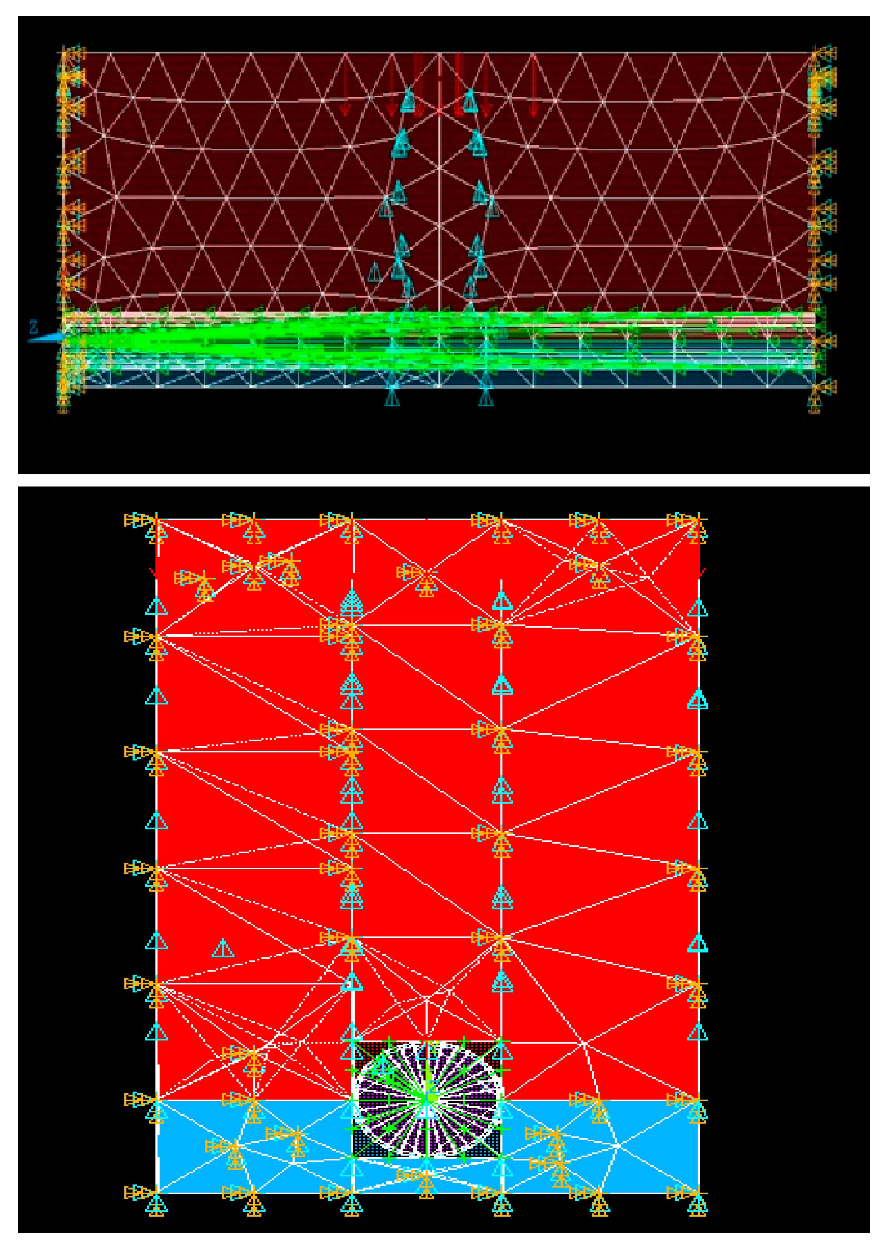
Moreover, for detecting the most critical state of static loading in this study, an active fault in the middle part of the concrete pipe is applied. Generally, in seismology, faults are divided into three main categories: active, semi-active, and inactive faults. The criterion for defining ground faults is the movement of their surface relative to each other. For instance, the fault slip ratio is approximately 1 cm each year which means that the fault slip is 20 cm over a 20-year activity. For this purpose, the slip with the movement of 20 cm is assumed in the middle of GPC pipes to evaluate fault behavior in this field. Therefore, for applying this displacement, the nodes on the right side of the fault are moved 0.1 m downwards and the nodes on the left side are moved 0.1 m upwards in Y-direction (Figure 9).
It is essential to point out that the dead loads on the underground pipeline are typically more efficient than the live loads. Because the efficacies of live load, which can be applied as traffic, are to diminish rapidly with the increment of soil depth. However, the live load may be more critical compared to dead loads for underground pipes at shallow depth [36,37]. In this study, the efficacy of live load on a GPC underground pipeline has been presented by using the details derived from the AASHTO standard which was used in previous studies. According to AASHTO, the spread area affected by the truckload has a length of 2 m and the width of 1.5 m considered in the middle part of the GPC pipe to the bearing performance of solid under static loading at failure moment [38]. Thus, the live load used for validating the numerical results will also be used which is calculated as follows:
- P = 50,000 lbs = 222,411 N;
- A = 2 × 1.5 = 3 m;
- Pressure (Live load) = 74,137 Pa (N/m2).
3.2. Seismic Loading
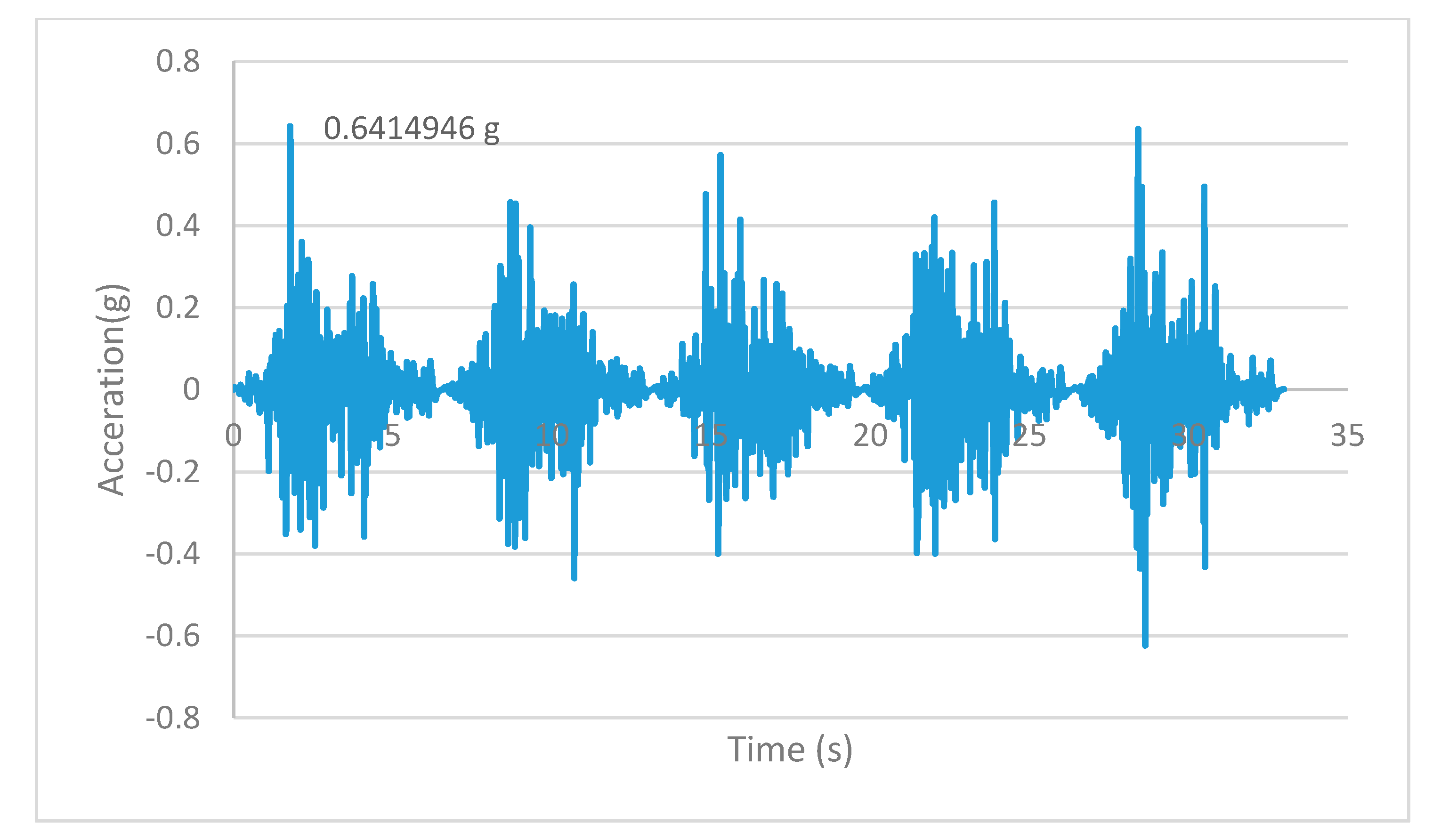
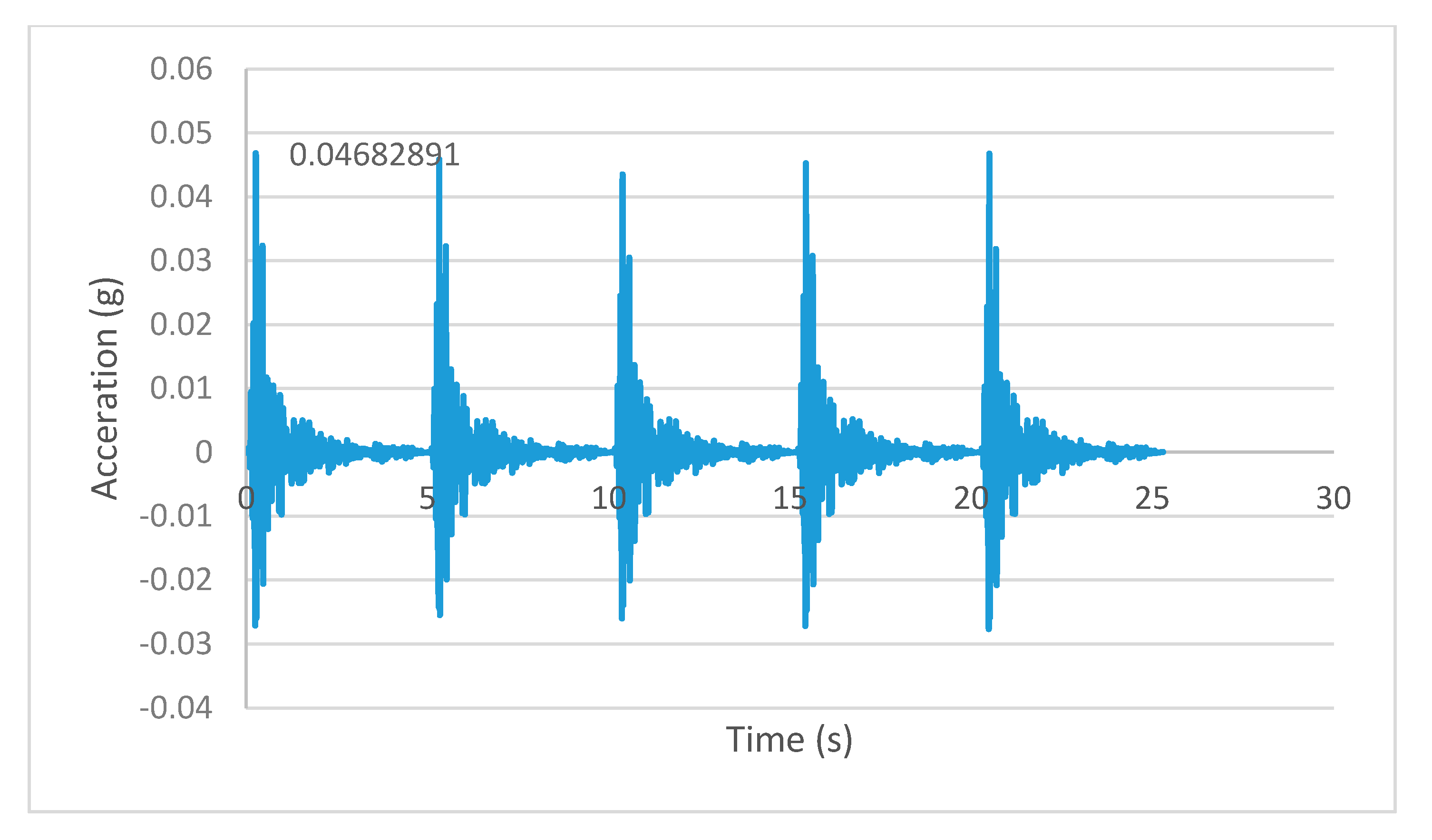
Once an earthquake occurs in a region, the diverse directions of ground motion are incensed due to stress waves in the ground. Generally, the changes of ground motion parameters, such as motion amplitude, frequency, and movement duration will happen as seismic waves pervade the overlying soil and become deflected when reaching the surface [39,40]. According to the study by Prasad [41], the range of predominant frequencies for most earthquakes resulting in crucial damage is between 1 to 2 Hz along with an acceleration which has an amplitude around 0.5 g. On the other hand, Wu [42] discussed the mechanism of earthquakes, and the nature of the movements is not radically attributed to the previous earthquakes as changes in the earth crust would not have rapidly appeared. In the FE software (ANSYS), seismic records of each earthquake are commonly described through acceleration, velocity, and displacement for each structure. Since the interaction between soil and structure is to be evaluated through obtaining the optimal displacement of GPC pipes, two specific records of time-history ground motion belonging to the Tabas (Iran, 1978) and Friuli (Italy, 1981) Earthquakes have been considered to assess the effects of each earthquake on the response of the GPC pipe in this study. The peak value corresponding to the ground displacement which was applied by a series of harmonic components for the Tabas and Friuli earthquakes are 0.093 m and 0.025 m, respectively (Figure 10 and Figure 11). In addition, the acceleration generated by each earthquake is given as shown in Figure 12 and Figure 13. The former with the peak value of 0.6 g belongs to the Tabas earthquake and the latter with the approximate value of 0.046 is recorded for the Friuli earthquake. The typical static and seismic loadings are shown in Table 9.
3.3. Determination of the Critical Node for Evaluating the Displacement of GPC Buried Pipe under Applied Loads
The modeling strategy used in this study emphasizes more on the numerical results in previous investigations because of the lack of experimental observations regarding the downward displacement of the underground pipe. Qin et al. [44] argued that the uplift force which is twice the thrust force applied on the upper half of the pipe can be considered as the critical state under the equilibrium condition of applied loads for a numerical model of a buried pipe.
In addition, Yehia et al. [45] expressed a similar attitude that the maximum value of P/2 on the upper half of the pipe, which illustrates the acceptable satisfaction between numerical and experimental tests, can be considered as the critical state in the case of underground pipe displacement; hence, the node 20, located on the upper half and the middle length of GPC pipe, has been chosen for this purpose.
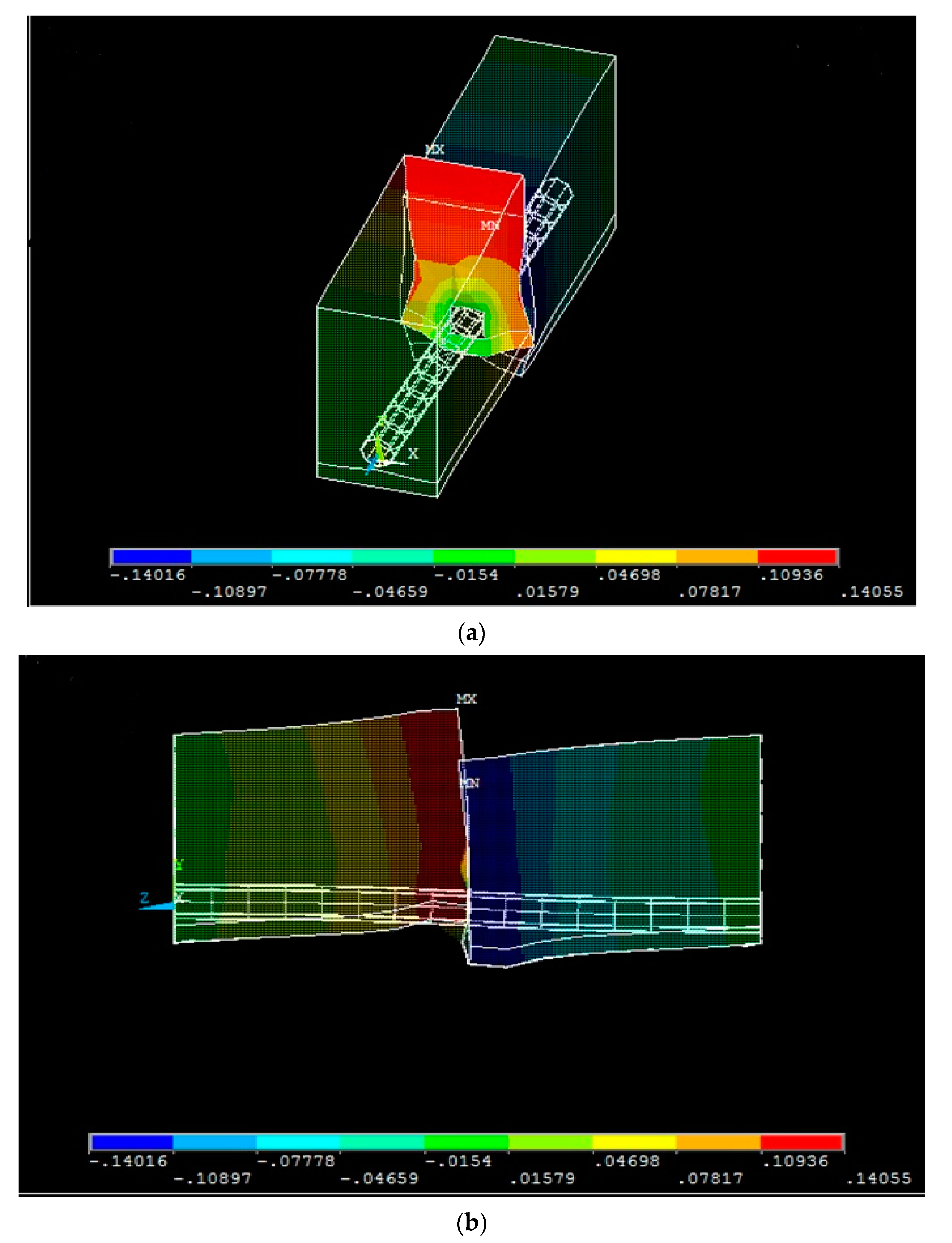
It does not necessarily mean that the displacement of the GPC pipe has been obtained in the FE software ANSYS without considering the settlement of the soil surrounding the GPC pipe. Indeed, the ANSYS software can provide the computed numerical results under diverse magnitude settlements between the settlement of soil and pipe proving the numerical results calculated by the FE method are in accordance with the concurrent movement of soil and GPC pipe. Furthermore, the deformation of the GPC pipe affects the deformed shape of the soil surrounding the GPC pipe due to simultaneous deformation of soil and pipe under static loading. Figure 14a is the isometric view of the GPC pipe and soil settlement, and Figure 14b is the side view of the FE model based on Figure 14a.
4. Boundary Condition
The boundary condition which can be recommended for the underground concrete pipe is fixed-support at two ends of the soil–GPC pipe model. Since the piping networks are very long, whereas the pipes have a 7.6 m length based on the standard AASHTO considered for this study, the pipe modeling will be reduced to the pipe with this standard length. Therefore, underground concrete pipes can be implemented, so that they are placed on the support which has been fastened with a mortar and rubber seal. In this state, it can be simulated as the fully fixed-support in ANSYS (Figure 15). The fixed-support embedded at the two ends of the concrete pipe can impede the vertical displacement of the bottom section of the GPC pipe and, subsequently, mortar and sealant can prevent the rotation and displacement of other regions of the concrete pipe [46,47]). On the other hand, the use of the GPC pipe based on the details of class ll nonreinforced concrete in ACAP standard, commonly used in industry, can minimize the efficacy of boundary conditions on the structural response of infrastructures. Hence, based on the above-mentioned statements and more compatibility of the simulated concrete pipe model in the FE software with the actual concrete pipe applied in the industry, the fully fixed-support has been recommended as a boundary condition in this study.
5. Discussion about Optimal Mesh Size of GPC Pipe
Generally, the proper number of elements and optimal meshing for more convergence in the numerical analysis of structures are commonly two key points that have been considered in FEM. According to the previous numerical studies, it was found that a large number of elements can have a notable effect on the achieved numerical results to be exaggerated, even though the improvement of computed results is typically attributed to the use of a fine mesh in FEM; however, this attitude is not always defensible. Lee [36] claimed that several numerical results by fine-meshed elements could not be calculated by the FE software, as the notable computation time around one day or more is desired for this purpose.
According to the above explanation, the following conclusions are drawn to determine the optimal mesh size of elements used in this study:
- ➢
- The elements with the mesh sizes of 1, 075, 0.5, and 0.25 m are used for FE analysis of the model including two soil types and the GPC pipe with a length of 7.6 m;
- ➢
- It is observed that the numerical results of 0.5 m and 0.25 m are obtained without significant variations compared to those of 1 m and 0.75 m. The convergence analysis for identifying the proper mesh size is the most important method to reduce the error related to the achieved force and displacement results in FE as the FE model with a fine mesh makes the numerical calculations more accurate compared to a coarse mesh. On the other hand, Weck and Nottebaum [48] discussed that it is predictable that the errors with a higher number of elements in the FE model need to converge nearly to zero. Accordingly, the numerical results in the relation to displacement and force have high accuracy with the enhancement of element numbers in FE models [48,49]. Thus, the mesh size of 0.5 including 3725 elements has been chosen for the FEM of the GPC pipe model. In addition, the numbers corresponding to the material properties defined in ANSYS are given in Table 10.
6. Static and Seismic Analysis
The analysis types are typically categorized into two groups involving static and seismic analysis. In this investigation, the static analysis will be conducted by using a self-weight of soil and pipeline as dead load, traffic loads based on AASHTO standard as live load, internal fluid pressure in the GPC pipe, and fault displacement in the middle length of GPC pipe.
As regards the seismic analysis, the seismic load based on displacement records with 0.6 g and 0.047 g of ground acceleration presented in Figure 10, Figure 11, Figure 12 and Figure 13 and Table 9 from the TABAS and Friuli earthquakes will be applied to the model of the GPC pipe to compute the seismic analysis in this study.
6.1. Static Analysis of GPC Underground Pipe
In this study, the static analysis is executed by employing the 7.6-m model of the GPC pipe under static loadings (Figure 5) which are self-weight of the GPC pipe and soil, traffic load onto the ground, internal fluid pressure, and fault displacement in the middle position of the GPC pipe. The main reason for applying such a load combination is to evaluate the most critical statement of the GPC pipe at the failure moment. The self-weight of both the GPC pipe and soil is calculated by applying the gravity (9.81 N) to the created FE model in ANSYS. As shown in Table 9, the applied traffic load is used as the uniform contact pressure with the value of 74,137 N/m2 on the top surface of the backfill soil which is exactly located on the fault considered in the middle position of the GPC pipe as well (Figure 16). In addition, node no. 20 in the element is chosen as the most critical node for this purpose. The internal pressure of 414 KPa is also applied to the internal surface of the GPC pipe model. It is urgent to point out that the mechanical properties of the GPC pipe, such as the compressive strength and density made from PC with diverse dosages of 0, 10, 20, 30, 50, and 70% FA as replacement of PC weight were experimentally obtained in this study (Table 11, Table 12 and Table 13), along with the 9 parameters related to the nonlinear state of the GPC calibrated in this investigation (Table 14) [3,50].
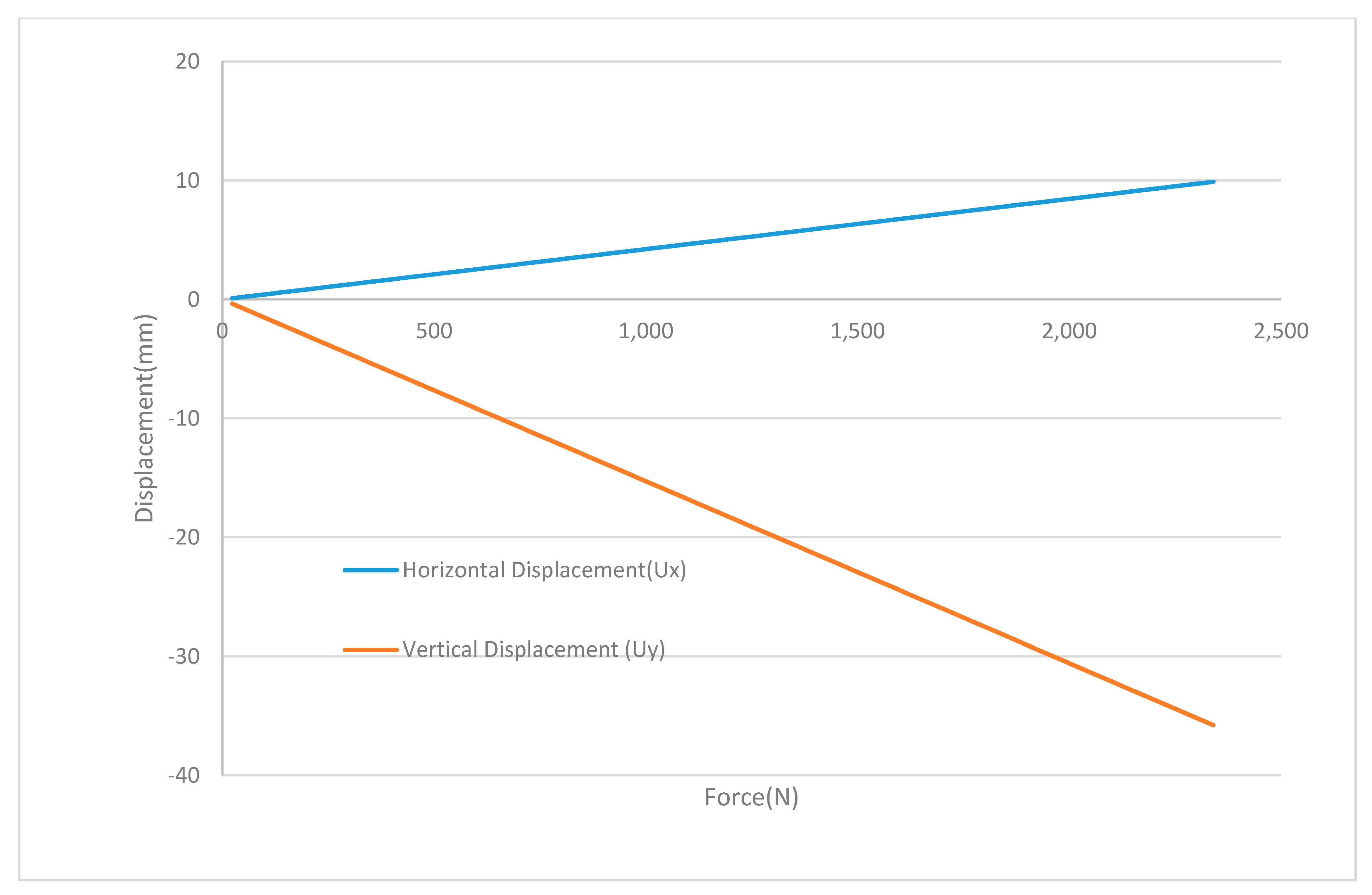
The typical vertical displacement of the buried GPC pipe under static loading is presented in Figure 17. Two types of vertical and horizontal displacements are to be assessed for GPC pipes with the variety of FA content with the dosages of 0, 10, 20, 30, 50, 70% as the replacement of PC weight on the directions of the y- and x-axis, respectively. It is assumed that the GPC pipe model has no slip in the direction of the z-axis.
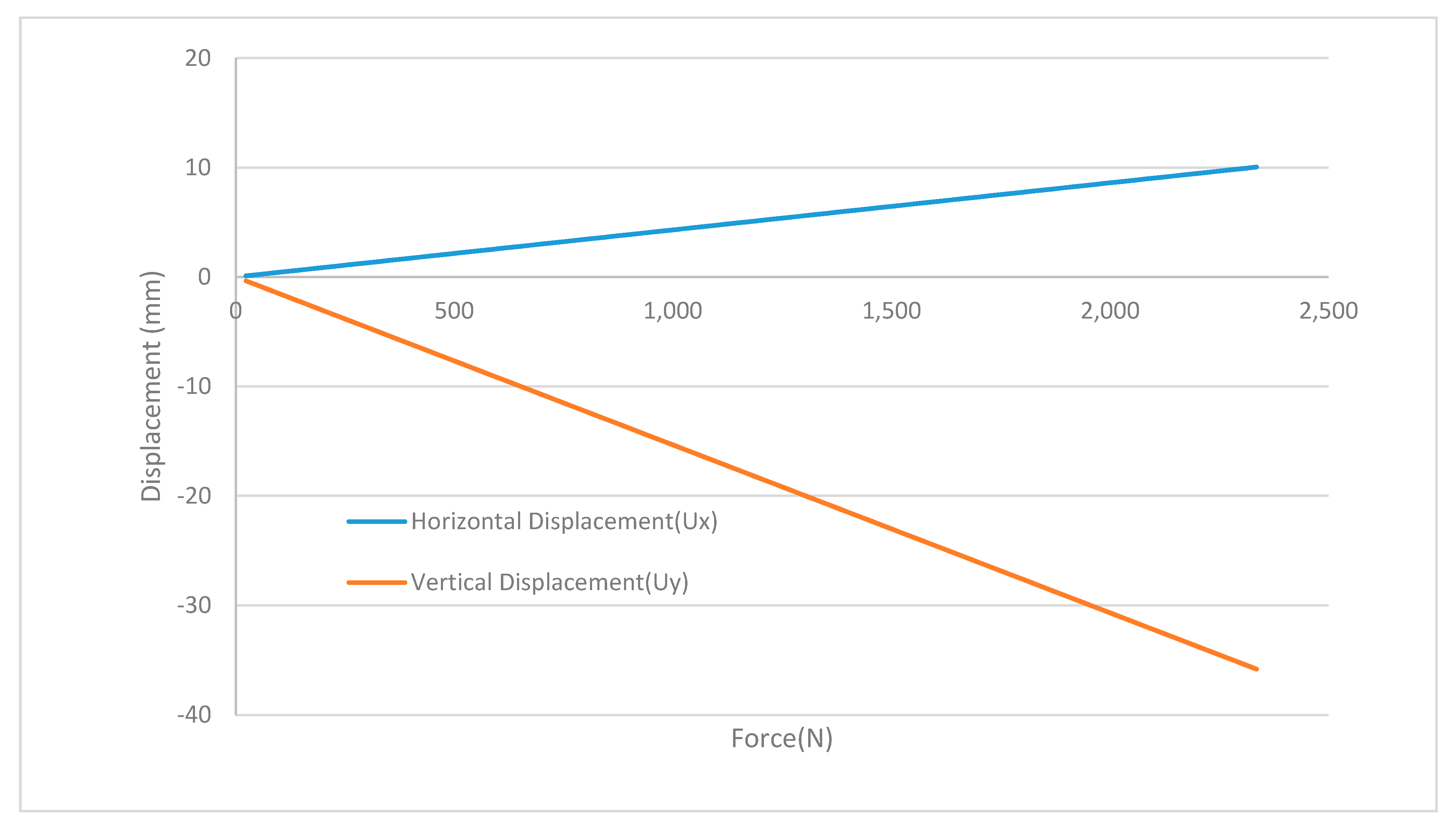
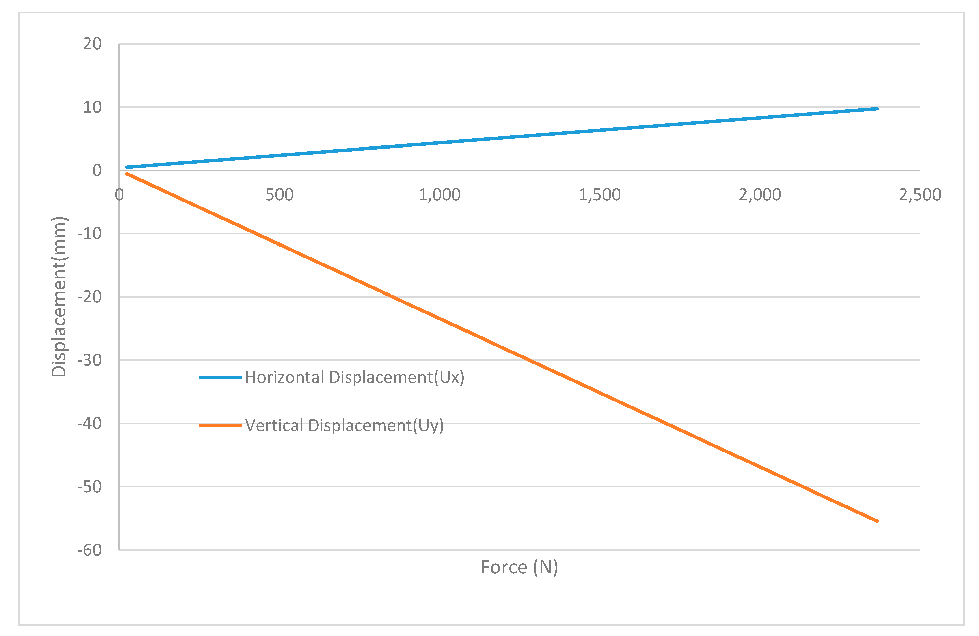
The movement of the GPC underground pipe is in coordination with soil under static loadings. It is possible to assess that the magnitude of the vertical displacement for the GPC pipe with diverse dosages of FA is commonly less than that of the horizontal displacement when comparing the force–displacement graphs which are shown in Figure 18, Figure 19, Figure 20, Figure 21, Figure 22 and Figure 23. Indeed, Figure 18, Figure 19, Figure 20, Figure 21, Figure 22 and Figure 23 demonstrate the comparison of the GPC pipe response for both vertical and horizontal displacements with the values of 0% to 70% FA as a raw material of the GPC pipe in which the compressive strength of this concrete type is experimentally examined in this study (Table 11, Table 12 and Table 13) and other equivalent parameters are also defined in the model (Table 14). These graphs demonstrate that the vertical displacement of GPC pipes subjected to static loading is much higher in comparison with the horizontal displacement of underground GPC pipes. Figure 18 shows that the variation of the vertical displacement for the GPC pipe with 0% FA as benchmark case is 0.035842 m which is roughly 3.56 times the amount of the horizontal displacement. In addition, Figure 23 shows a significantly higher vertical displacement in the FE analysis under static loadings for the GPC pipe with 70% FA, so that, the vertical displacement is 5.67 times the horizontal displacement. The values of vertical and horizontal displacements for this GPC pipe model are 0.055327 m and 0.009748 m, respectively. For numerical simulations of GPC pipes with 10%, 20%, 30%, and 50% FA, based on Figure 19, Figure 20, Figure 21 and Figure 22, it is found that the values of the vertical displacement for 10% and 20% are 1.92 times compared to horizontal displacements showing no change with adding the FA content by 10%, whereas the GPC pipe model including 30% FA has a vertical displacement which is 3.61 times the horizontal displacement. This trend is dramatically enhanced for the GPC pipe involving 50% FA so that the values subjected to a vertical displacement are approximately 5.7 times those of the horizontal displacement.
Eventually, the optimal performance of the underground GPC pipe, as the lowest vertical and horizontal displacements under static loadings, is numerically achieved for the FE model with the inclusion of 20% FA among all the GPC mix designs investigated in this study (Figure 24). Hence, This FE model with 20% FA content has been considered for dynamic (time-history) analysis in the next part. So, two types of material properties for the GPC pipe will be defined under seismic loading which are the FE models with 0% and 20% as control and benchmark specimens, respectively.
6.2. Dynamic Analysis of GPC Underground Pipe
After weighing up all methods of the transient dynamic analysis (time-history), it seems that the full-time method can certainly offer more benefits than the other methods. Indeed, the unlimited application of all nonlinear behaviors and the utilization of various loads such as non-zero displacements are two superior features that distinguish the full-time method from the other methods numerically utilized in the previous studies. Thus, the decision is made to employ the full-time method in the time-history analysis of the GPC pipe through the ANSYS platform. Further explanations in the case of the full-time method will be illuminated in the following points [51,52,53,54,55]:
- All linear and nonlinear properties of geometric material and linear and nonlinear elements are applicable. Young’s modulus and density are the minimum properties of the material to be determined.
- The first loading in the transient dynamic analysis (time history) is typically performed to provide the initial conditions governing the model in a very short time. Subsequently, the settings subjected to the main loading are to be conducted in continuation of the first solution.
- The effects of temporal integration must be active in transient dynamic analyses with damping effects or inertial loads. Otherwise, the problem is solved in static mode. This option is commonly active by default in the ANSYS software.
- The effect of stress stiffening is typically active by default, except that the following two cases can be inactive:
- ➢
- Dynamic analysis is performed in a linear state;
- ➢
- It should be ensured that the structure is not in the range of its buckling load and does not suffer from buckling due to the applied load.
The 7.6-m model comprising soil and the GPC pipe is employed for executing the transient (time history) analysis under the seismic loading described by the Tabas earthquake. The peak values corresponding to the displacement time series and acceleration data, released from Peer Nga Storing Motion Database Record (PNSMDR), are around 0.092 m and 0.64 g, respectively. In this section, the displacements related to seismic loading and other relevant forces such as acceleration in X-direction and reaction force at node 1 are analyzed through the ANSYS software to distinguish the most critical state in the nonlinear performance of the GPC underground pipe throughout the occurrence of an earthquake. Since the number of maximum time steps in the ANSYS platform is 1000. Beyond that, the specific command and the powerful finite element software for commercial purposes are required without the limitations of the FE software available in the academic community due to the high computational time. Thus, this FE model is analyzed under the effect of the Tabas earthquake with 3-s duration as the number of rows in the text file is 300 given that 3 s from the record of the Tabas earthquake with the time step of 0.01 equals 300.
The only route for recognizing the critical region of GPC pipe interacting with two types of soils for both static and seismic analysis is node 20 located in the crown on the upper half of the GPC pipe in the middle span of the buried pipe. Indeed, the significant aim in this section is to compare the response of the GPC underground pipe under the applied seismic loading for both GPC mix designs with the inclusion of 20% FA as a PC replacement and 0% FA as the benchmark in this study. It is essential to note that there is a limitation about the depth of the GPC pipe as the width and depth of sidefill and backfill, two soil types used in this study, are arranged under ACPA and AASHTO standards. In addition, it is assumed that the boundary condition of the fixed-support is similar to static analysis.
6.3. The Response of GPC Pipe under Seismic Loadings for Critical State
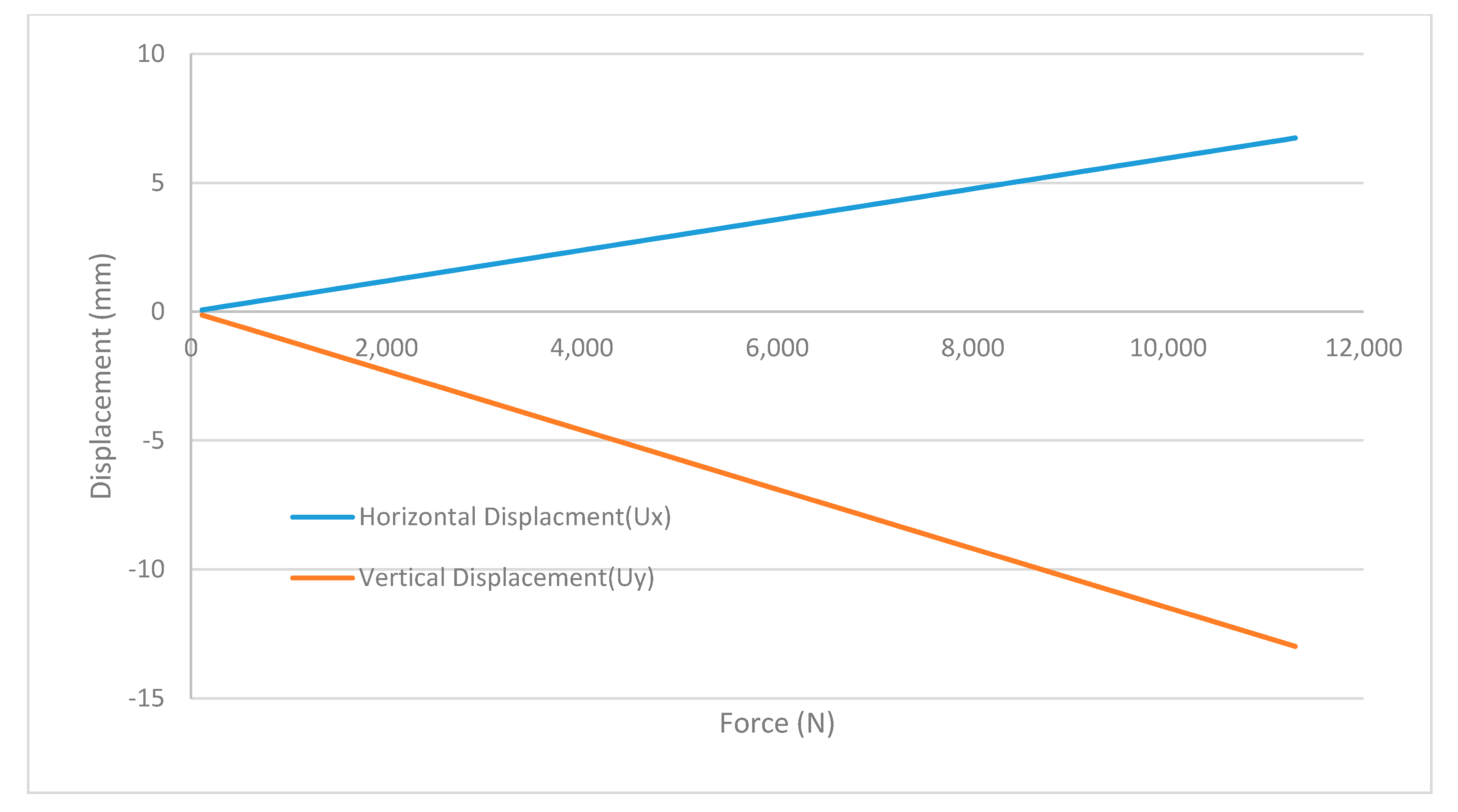
The numerical results of the time-history analysis are presented for the induced crown displacement on the upper half of the GPC pipe due to applying the records related to the Tabas earthquake with the peak value of 0.092 m (Figure 10). It is worth noting that the developed model predicts the crown displacement of the GPC pipe with excellent precision. A comprehensive attempt is made at this point to simulate the FE model exactly based on the existing reality in the construction industry considering the valid standards such as ACPA and AASHTO regarding the soil properties and pipe geometry. Based on Figure 25, it can be seen that the maximum value of vertical displacement for the GPC pipe with 0% FA is approximately 0.145 m which is higher than that of GPC pipe with 20% FA with the reduced value of 0.1339 m showing the percentage difference of 8%. Furthermore, the developed FE model enables the prediction of the tendency of the displacement–time relationship as obviously indicated in Figure 25.
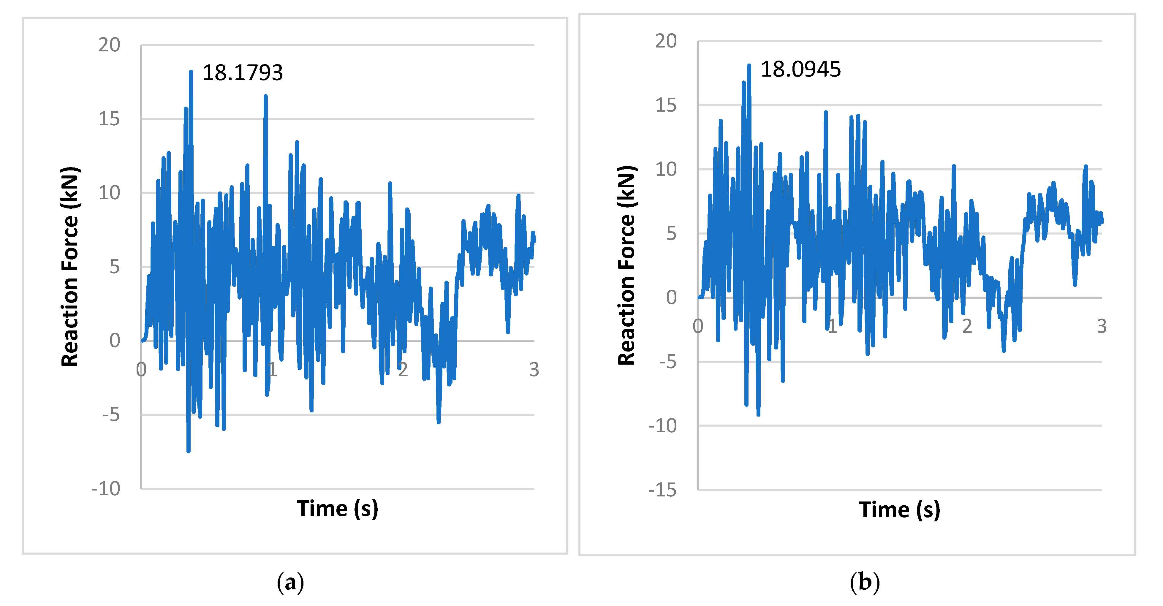
In the case of horizontal displacement, it can be found that there is no remarkable change between two types of the GPC pipe model containing 20% and 0% FA so that the maximum amount of horizontal displacement for the GPC pipe without FA content is around 2.6% higher than that of the GPC pipe model with 20% FA (Figure 26). However, these values belonging to vertical and horizontal displacements of the FE model under seismic loadings are much higher compared to the data corresponding to the static analysis numerically investigated. In addition, node 1 with the coordinates of x = 0, y = 0, z = 0 has been chosen to evaluate the performance of fixed-support at two ends of the GPC pipe under seismic loadings in this study. The implication of these findings is presented in Figure 27. It can be seen that the maximum values subjected to the reaction force in fixed-support of the GPC pipe with 0% and 20% FA are 18,179.3 N and 18,094 N, respectively.
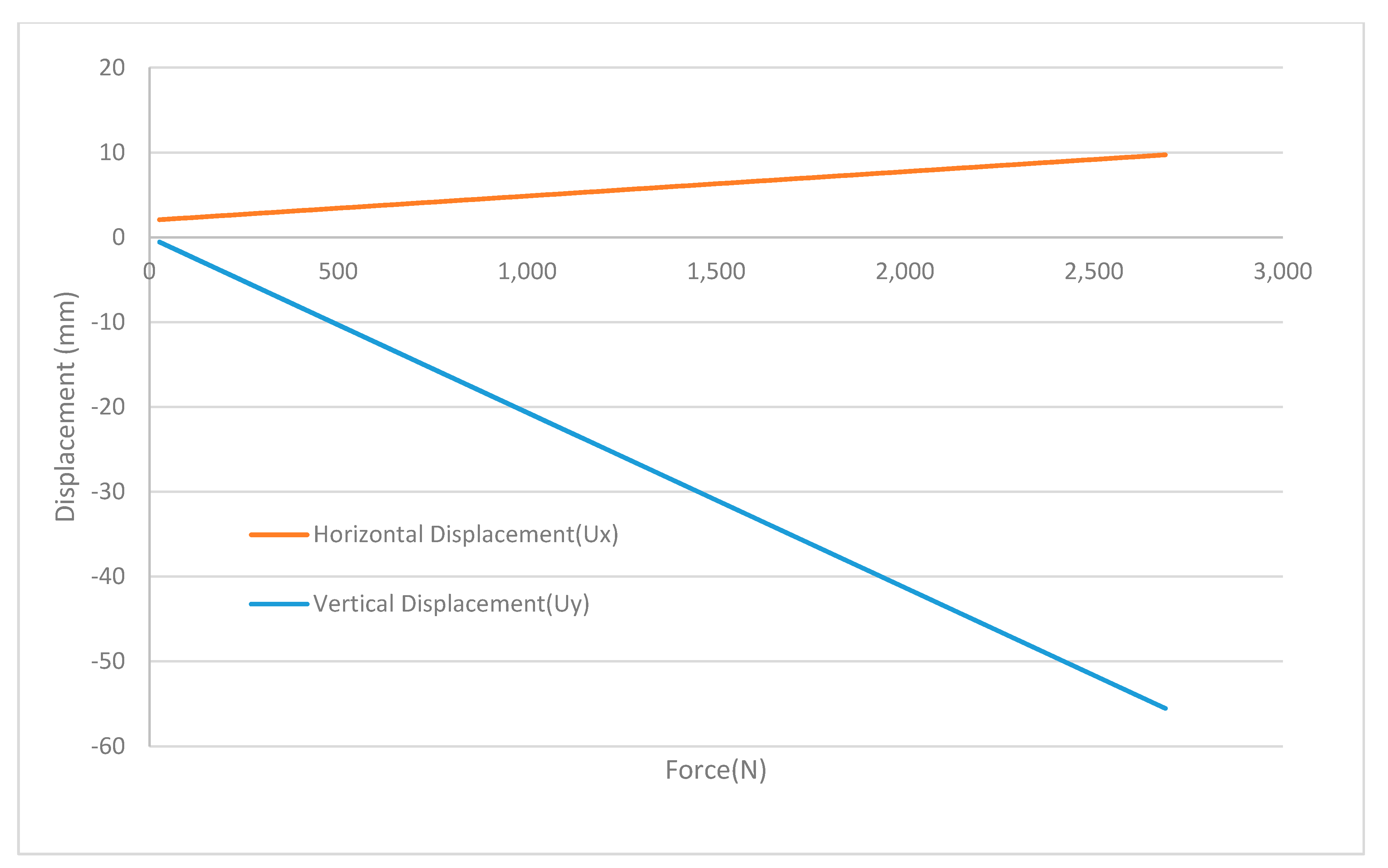
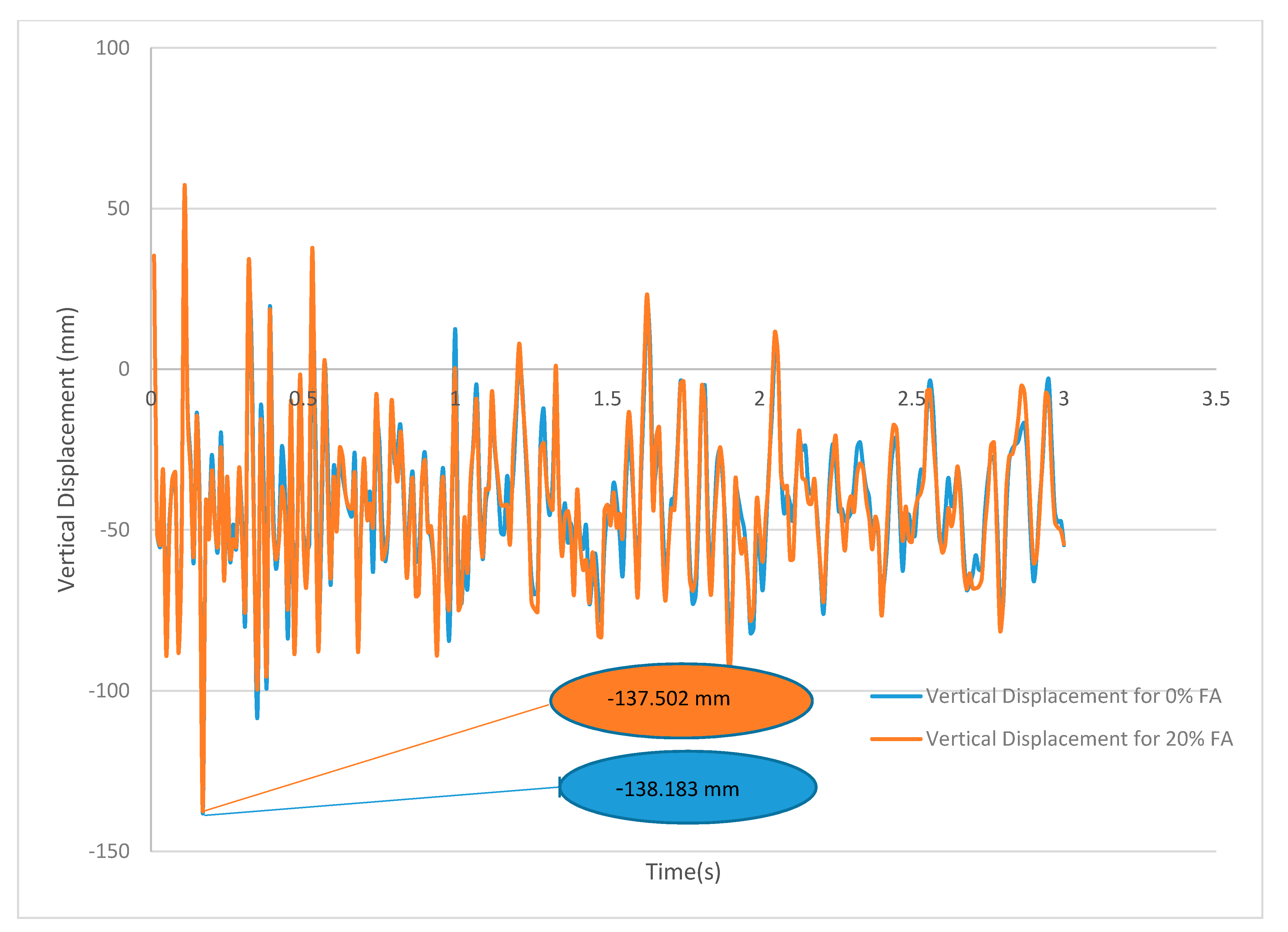
When comparing the above-mentioned results to those of other earthquakes, for instance, the Friuli earthquake that occurred in Italy (1981), it is useful to point out that a marginal reduction in the case of vertical displacement can be seen with what has previously been found for the Tabas earthquake. As shown in Figure 28, the vertical displacements after applying the records related to the Friuli earthquake are approximately 0.138 m and 0.137 m for underground pipes with the inclusion of 0% and 20% FA, respectively. However, no significant change was observed in the case of horizontal displacement between two types of buried pipe models (0% and 20% FA) under the seismic loading of the Friuli earthquake in Figure 29. Collectively, the results for the underground pipe under the two earthquakes with fully-distinctive data follow from the fact that the efficiency of FA as PC replacement in the decrement of pipe response, especially vertical displacement, under seismic loading with high acceleration is more tangible than that with a lower amount, given that the peak value of acceleration belonging to the Tabas earthquake is around 14 times the value corresponding to the Friuli earthquake.
7. Summary and Conclusions
In this study, the William–Warnke failure criterion and the modified Popovics model were presented for the nonlinear behavior of underground GPC pipes to illustrate the response of stress–strain for underground GPC pipes with diverse values of FA. To objectively evaluate the nonlinear performance of an underground GPC pipe exposed to static loading, the displacement of node no. 20 in element 1126 located in the region of the pipe crown is taken into account as the critical zone in the middle of the GPC pipe. The value of this displacement varies based on the material properties of the concrete with the variety of FA content defined in the FE model.
The following conclusions are drawn:
- ➢
- The numerical results of the static analysis demonstrate that the highest value of displacement occurs in the middle of the GPC in which traffic load and fault displacement were utilized as the two types of static loads in this study. The output of numerical results indicated that the dosage of FA in the range of 10–30% has a key role in the improvement of the optimal displacement in static analysis.
- ➢
- As regards the time-history analysis, based on the displacement records from two distinctive actual earthquakes (Tabas, Iran in 1979; Friuli, Italy in 1981), it was proved that the inclusion of FA in the GPC pipe has a significant role in the improvement of the vertical displacement in the underground model compared to horizontal displacement as it was observed in the static analysis as well.
- ➢
- In conclusion, it would appear that the role of FA on the improvement of the vertical response of the GPC pipe under seismic loading with high acceleration is more visible compared to the other earthquakes with low acceleration.
In addition, the assumptions and limitations used in this study are given as follows:
- ➢
- The concrete properties of the GPC pipe for linear and nonlinear behavior of the GPC pipe are based on the findings experimentally obtained in this study, such as compressive strength, density, and other parameters numerically validated in this field.
- ➢
- The trench simulated in the ANSYS platform is composed of stiff clay for bedding and sidefill soil along with silty clay for backfill soil.
Despite the fact that this study can distinguish the initial assessment regarding the response of a GPC pipe with various percentages of FA under static loading, further explorations including more details on significant factors and parameters as a key role in the development of GPC pipe response are needed.
As regards time-history analysis for seismic loading, the numerical results are widely accepted in case of the response of GPC pipe under seismic loading which can be considered as the great breakthroughs in this field; nevertheless, there are several limitations over the implementation of each step of the FE analysis. The major source of limitation is due to the lack of previous studies related to GPC pipes under seismic loading so that we are unable to compare the current findings with those in preliminary studies to reach the yield answer about the performance of this concrete pipe type against applied static and seismic loadings. Therefore, the necessity of utilizing a parametric study to identify the main factors playing a key role in the improvement of GPC pipe response as well as the quantitative evaluation of these parameters needs to be centralized in upcoming studies.
Author Contributions
Both authors (K.F.T. and S.M.) equally contributed to the present work. All authors have read and agreed to the published version of the manuscript.
Funding
This research received no external funding.
Institutional Review Board Statement
Not applicable.
Informed Consent Statement
Not applicable.
Data Availability Statement
The data reported in this study can be found in the sources cited in the reference list.
Conflicts of Interest
The authors declare no conflict of interest.
References
- Ghafoori, N.; Najimi, M.; Diawara, H.; Islam, M. Effects of class F fly ash on sulfate resistance of Type V Portland cement concretes under continuous and interrupted sulfate exposures. Constr. Build. Mater. 2015, 78, 85–91. [Google Scholar] [CrossRef]
- Shehab, H.K.; Eisa, A.; Wahba, A. Mechanical properties of fly ash based geopolymer concrete with full and partial cement replacement. Constr. Build. Mater. 2016, 126, 560–565. [Google Scholar] [CrossRef]
- Tee, K.F.; Mostofizadeh, S. Numerical and experimental investigation of concrete with various dosages of fly ash. AIMS Mater. Sci. 2021, 8, 587–607. [Google Scholar] [CrossRef]
- Mostofizadeh, S.; Tee, K.F. Utilization of Nonlinear Model for Finite Element Analysis of Reinforced Fly Ash Concrete Cubes and Beams. In Proceedings of the 40th Cement and Concrete Science Conference, Sheffield, UK, 31 August–4 September 2020. [Google Scholar]
- Tee, K.F.; Agba, I.F.; Samad, A.A.A. Experimental and Numerical Study of Green Concrete. Int. J. Forensic Eng. 2019, 4, 238–254. [Google Scholar] [CrossRef]
- Gharehbaghi, K.; Tee, K.F.; Gharehbaghi, S. Review of geopolymer concrete: A structural integrity evaluation. Int. J. Forensic Eng. 2021, 5, 59. [Google Scholar] [CrossRef]
- Tee, K.F.; Mostofizadeh, S. A Mini Review on Properties of Portland Cement Concrete with Geopolymer Materials as Partial or Entire Replacement. Infrastructures 2021, 6, 26. [Google Scholar] [CrossRef]
- Alzabeebee, S.; Chapman, D.N.; Faramarzi, A. A comparative study of the response of buried pipes under static and moving loads. Transp. Geotech. 2018, 15, 39–46. [Google Scholar] [CrossRef]
- Mohamedzein, Y.E.-A.; Al-Aghbari, M.Y. Experimental study of the performance of plastic pipes buried in dune sand. Int. J. Geotech. Eng. 2016, 10, 236–245. [Google Scholar] [CrossRef]
- Ebenuwa, A.U.; Tee, K.F. Reliability estimation of buried steel pipes subjected to seismic effect. Transp. Geotech. 2019, 20, 100242. [Google Scholar] [CrossRef]
- Chaallal, O.; Arockiasamy, M.; Godat, A. Field Test Performance of Buried Flexible Pipes under Live Truck Loads. J. Perform. Constr. Facil. 2015, 29, 04014124. [Google Scholar] [CrossRef]
- Rakitin, B.; Ming, X. Centrifuge Modeling of Large Diameter Underground Pipes Subjected to Heavy Traffic Loads. Bulletin of South Ural State University series. Constr. Eng. Archit. 2016, 16, 31–46. [Google Scholar]
- MacDougall, K.; Hoult, N.A.; Moore, I.D. Measured load capacity of buried reinforced concrete pipes. ACI Struct. J. 2016, 113, 63–73. [Google Scholar] [CrossRef] [Green Version]
- Lay, G.; Brachman, R. Full-scale physical testing of a buried reinforced concrete pipe under axle load. Can. Geotech. J. 2014, 51, 394–408. [Google Scholar] [CrossRef]
- McGrath, T.J.; DelloRusso, S.J.; Boynton, J. Performance of Thermoplastic Culvert Pipe Under Highway Vehicle Loading. In Proceedings of the Pipeline Division Specialty Conference, Cleveland, OH, USA, 4–7 August 2002. [Google Scholar]
- Li, Y.; Song, G.; Cai, J. Mechanical Response Analysis of Airport Flexible Pavement above Underground Infrastructure under Moving Wheel Load. Geotech. Geol. Eng. 2017, 35, 2269–2275. [Google Scholar] [CrossRef]
- Neya, B.N.; Ardeshir, M.A.; Delavar, A.A.; Bakhsh, M.Z.R. Three-Dimensional Analysis of Buried Steel Pipes under Moving Loads. Open J. Geol. 2017, 7, 1–11. [Google Scholar] [CrossRef] [Green Version]
- Tee, K.F.; Wordu, A.H. Burst strength analysis of pressurized steel pipelines with corrosion and gouge defects. Eng. Fail. Anal. 2020, 108, 104347. [Google Scholar] [CrossRef]
- Fan, K.; Li, D.; Damrongwiriyanupap, N.; Li, L.-Y. Compressive stress-strain relationship for fly ash concrete under thermal steady state. Cem. Concr. Compos. 2019, 104, 103371. [Google Scholar] [CrossRef]
- Nath, P.; Sarker, P. Flexural strength and elastic modulus of ambient-cured blended low-calcium fly ash geopolymer concrete. Constr. Build. Mater. 2017, 130, 22–31. [Google Scholar] [CrossRef] [Green Version]
- Waqas, R.M.; Butt, F.; Zhu, X.; Jiang, T.; Tufail, R.F. A Comprehensive Study on the Factors Affecting the Workability and Mechanical Properties of Ambient Cured Fly Ash and Slag Based Geopolymer Concrete. Appl. Sci. 2021, 11, 8722. [Google Scholar] [CrossRef]
- Isojeh, B.; El-Zeghayar, M.; Vecchio, F.J. Simplified Constitutive Model for Fatigue Behavior of Concrete in Compression. J. Mater. Civ. Eng. 2017, 29, 04017028. [Google Scholar] [CrossRef] [Green Version]
- Halahla, A.M. Identification of Crack in Reinforced Concrete Beam Subjected to Static Load Using Non-linear Finite Element Analysis. Civ. Eng. J. 2019, 5, 1631–1646. [Google Scholar] [CrossRef] [Green Version]
- Popovics, S. A numerical approach to the complete stress-strain curve of concrete. Cem. Concr. Res. 1973, 3, 583–599. [Google Scholar] [CrossRef]
- Popovics, S. A review of stress-strain relationships for concrete. ACI J. 1970, 67, 243–248. [Google Scholar]
- Mander, J.B.; Priestley, M.J.N.; Park, R. Theoretical Stress-Strain Model for Confined Concrete. J. Struct. Eng. 1988, 114, 1804–1826. [Google Scholar] [CrossRef] [Green Version]
- EN 1992-1-1 (2004): Eurocode 2: Design of Concrete Structures—Part 1-1: General Rules and Rules for Buildings. Available online: https://www.phd.eng.br/wp-content/uploads/2015/12/en.1992.1.1.2004.pdf (accessed on 21 October 2021).
- Zamanian, S. Probabilistic Performance Assessment of Deteriorating Buried Concrete Sewer Pipes. Master’s Thesis, The Ohio State University, Columbus, OH, USA, 2016. [Google Scholar]
- ANSYS Inc. ANSYS User Manuals Released 13.0; ANSYS Inc.: Canonsburg, PA, USA, 2010. [Google Scholar]
- Kwan, A.; Dai, H.; Cheung, Y. Non-Linear Seismic Response of Reinforced Concrete slit shear walls. J. Sound Vib. 1999, 226, 701–718. [Google Scholar] [CrossRef]
- Terec, L.; Bugnariu, T.; Păstrav, M. Nonlinear analysis of reinforced concrete frames strengthened with infilled walls. Rom. J. Mater. 2010, 40, 214–221. [Google Scholar]
- Kachlakev, D.; Miller, T.; Yim, S. Finite Element Modeling of Reinforced Concrete Structures Strengthened with FRP Laminates; Oregon Department of Transport: Salem, OR, USA, 2001. [Google Scholar]
- Badiger, N.S.; Malipatil, K.M. Parametric Study on Reinforced Concrete Beam using ANSYS. Civ. Environ. Res. 2014, 6, 88–94. [Google Scholar]
- Mostofizadeh, S.; Tee, K.F. Evaluation of Impact of Fly Ash on the Improvement on Type II Concrete Strength. In Proceedings of the 39th Cement and Concrete Science Conference, Bath, UK, 9–10 September 2019; pp. 190–193. [Google Scholar]
- ACPA (American Concrete Pipe Association). Concrete Pipe and Box Culvert Installation Design Manual; American Concrete Pipe Association: Irving, TX, USA, 2007. [Google Scholar]
- Lee, H. Finite Element Analysis of a Buried Pipeline. Master’s Thesis, University of Manchester, Manchester, UK, 2010. [Google Scholar]
- Nath, P. The effect of traffic loading on buried pipes. In Soil-Structure Interaction: Numerical Analysis and Modelling; John, W.B., Ed.; E & FN Spon: London, UK, 1994. [Google Scholar]
- Moore, I.D.; Hoult, N.A.; MacDougall, K. Establishment of Appropriate Guidelines for Use of the Direct and Indirect Design Methods for Reinforced Concrete Pipe; AASHTO Standing Committee on Highways: Washington, DC, USA, 2014. [Google Scholar]
- Wang, L.R.L.; Raymond, C.Y.F. Seismic design criteria for buried pipelines. In Pipelines in Adverse Environments—A State of The Art; American Society of Civil Engineers: New York, NY, USA, 1979. [Google Scholar]
- Ebenuwa, A.U.; Tee, K.F. Reliability Analysis of Buried Pipes with Corrosion and Seismic Impact. In Proceedings of the 6th Symposium on Geo-Risk 2017, Denver, CO, USA, 4–7 June 2017; pp. 424–433. [Google Scholar]
- Prasad, S.K.; Towhata, I.; Ghandradhara, G.P.; Nanjundaswamy, P. Shaking table tests in earthquake geotechnical engineering. Geotechnics and Earthquake Hazards. Curr. Sci. 2004, 87, 1398–1404. [Google Scholar]
- Wu, T.H. Soil Dynamics; Allyn and Bacon: Boston, MA, USA, 1971. [Google Scholar]
- Peer Data Motion Database. 2020. Available online: https://ngawest2.berkeley.edu/ (accessed on 21 October 2021).
- Qin, X.; Ni, P.; Du, Y.-J. Buried rigid pipe-soil interaction in dense and medium sand backfills under downward relative movement: 2D finite element analysis. Transp. Geotech. 2019, 21, 100286. [Google Scholar] [CrossRef]
- Akl, A.Y.; Maher, M.M.; Metwally, K.G. Advance Analysis of Concrete Pipe-Soil Interaction. J. Eng. Appl. Sci. 2004. Available online: https://www.researchgate.net/publication/273763693_ADVANCED_ANALYSIS_OF_CONCRETE_PIPE-SOIL_INTERACTION/stats (accessed on 20 April 2021).
- Prombandankul, W.; Smittakorn, W. Compression-Shear Behavior and Water Impermeability of Rubber Seal in Precast Concrete Structures. Eng. J. 2020, 24, 137–148. [Google Scholar] [CrossRef]
- Das, B.; Sobhan, K. Principles of Geotechnical Engineering. Stamford: Cengage Learning. 2014. Available online: https://cdn.prexams.com/4863/principles_of_geotechnical_engineering_si_8e_solutions_manual.pdf (accessed on 30 November 2021).
- Weck, M.; Nottebaum, T. Adaptive meshing—Saving computational costs during the optimization of composite structures. Struct. Multidiscip. Optim. 1993, 6, 108–115. [Google Scholar] [CrossRef]
- Baiges, J.; Chiumenti, M.; Moreira, C.A.; Cervera, M.; Codina, R. An adaptive Finite Element strategy for the numerical simulation of additive manufacturing processes. Addit. Manuf. 2021, 37, 101650. [Google Scholar] [CrossRef]
- Tee, K.F.; Mostofizadeh, S. An Experimental Study of the Effects of Low-Calcium Fly Ash on Type II Concrete. Ceramics 2021, 4, 43. [Google Scholar] [CrossRef]
- Bathe, K.J.; Saunders, H. Finite Element Procedures in Engineering Analysis. J. Press. Vessel. Technol. 1984, 106, 421–422. [Google Scholar] [CrossRef]
- Hughes, T. Finite Element Method; Dover Publications: Mineola, NY, USA, 2012. [Google Scholar]
- Luo, Z.; Jiang, W. A reduced-order extrapolated technique about the unknown coefficient vectors of solutions in the finite element method for hyperbolic type equation. Appl. Numer. Math. 2020, 158, 123–133. [Google Scholar] [CrossRef]
- Sun, P.; Yang, H.; Deng, Y. Complex mode superposition method of non proportionally damped linear systems with hysteretic damping. J. Vib. Control 2020, 27, 1453–1465. [Google Scholar] [CrossRef]
- Yavuz, Ş.; Akdağ, M.; Karagülle, H. A fast processing method to perform transient analysis for vibration control. Simul. Model. Pract. Theory 2020, 104, 102152. [Google Scholar] [CrossRef]
Figure 1.
Parameter ‘n’ at different temperatures.
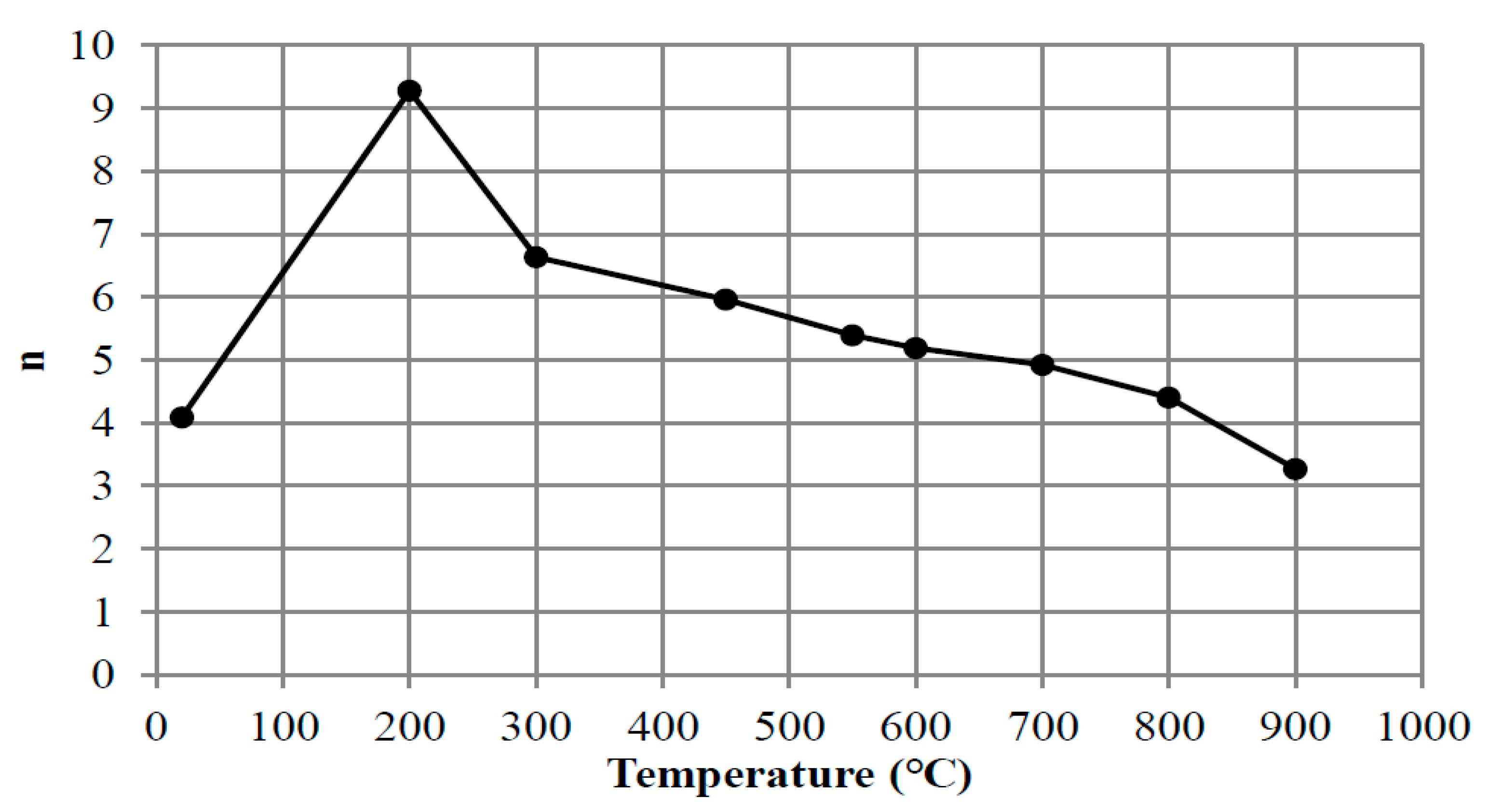
Figure 2.
Comparison of stress–strain relations and FE presented in this study for a concrete cube including 20% FA with the proposed equation of Ec= for modified Popovics models.
Figure 2.
Comparison of stress–strain relations and FE presented in this study for a concrete cube including 20% FA with the proposed equation of Ec= for modified Popovics models.

Figure 3.
Comparison of stress–strain relations and FE presented in this study for a concrete cube including 20% FA with the proposed equation of Ec = 2.5 for modified Popovics models.
Figure 3.
Comparison of stress–strain relations and FE presented in this study for a concrete cube including 20% FA with the proposed equation of Ec = 2.5 for modified Popovics models.

Figure 4.
(a) 2D and (b) 3D original pipe models in ANSYS based on Zamarian [28].
Figure 4.
(a) 2D and (b) 3D original pipe models in ANSYS based on Zamarian [28].
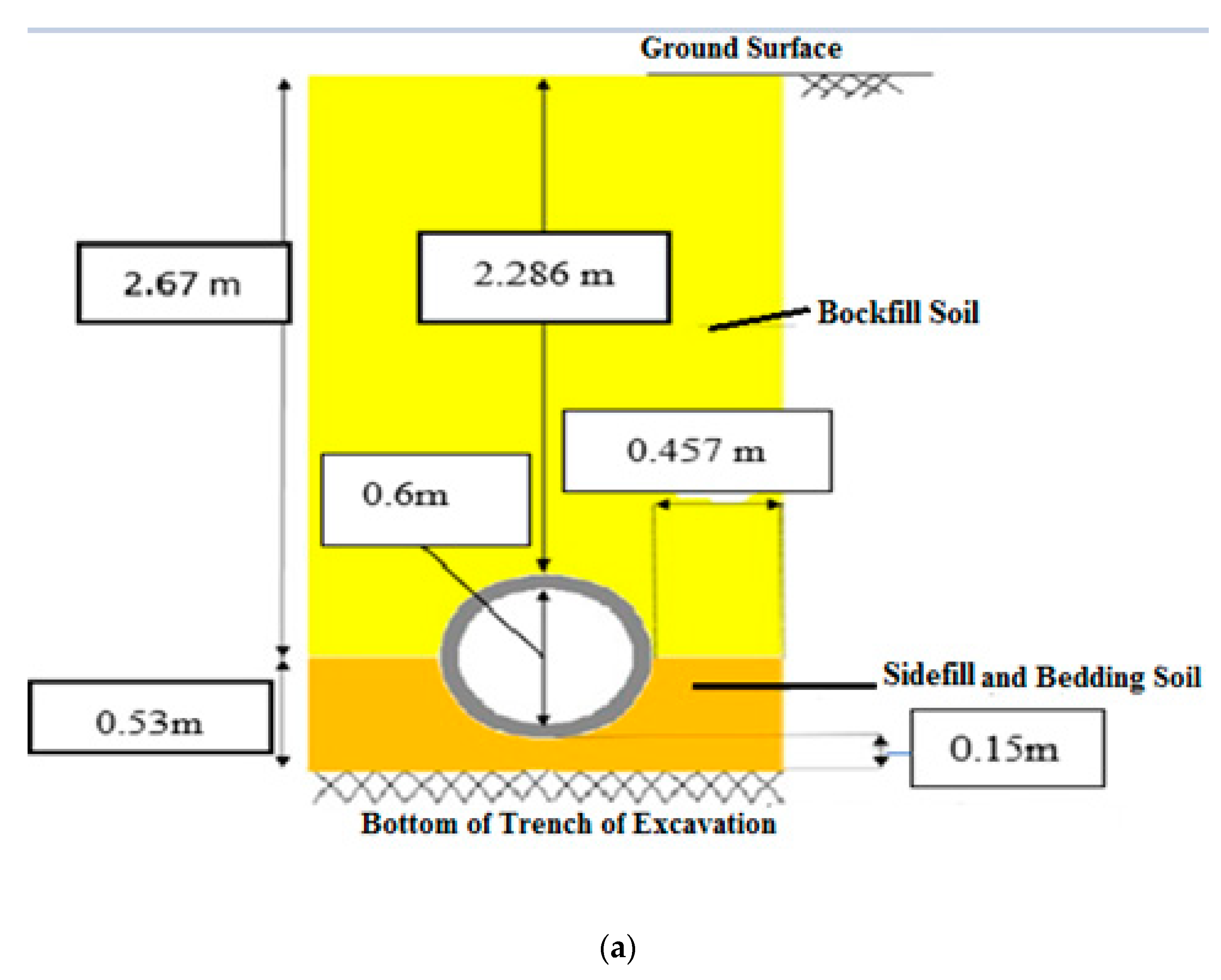
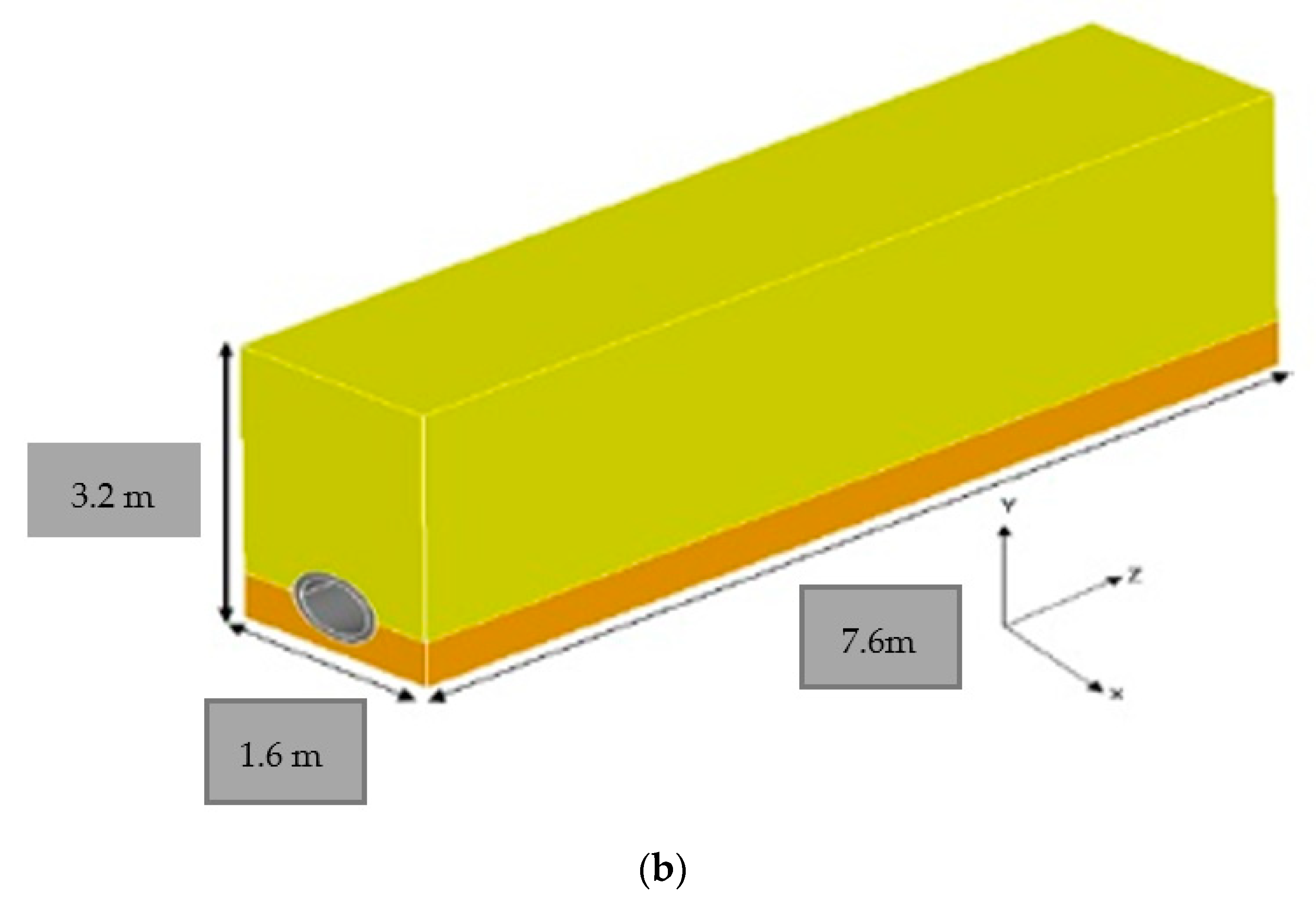
Figure 5.
(a) 2D and (b) 3D pipe models in ANSYS 18.2 (current study).
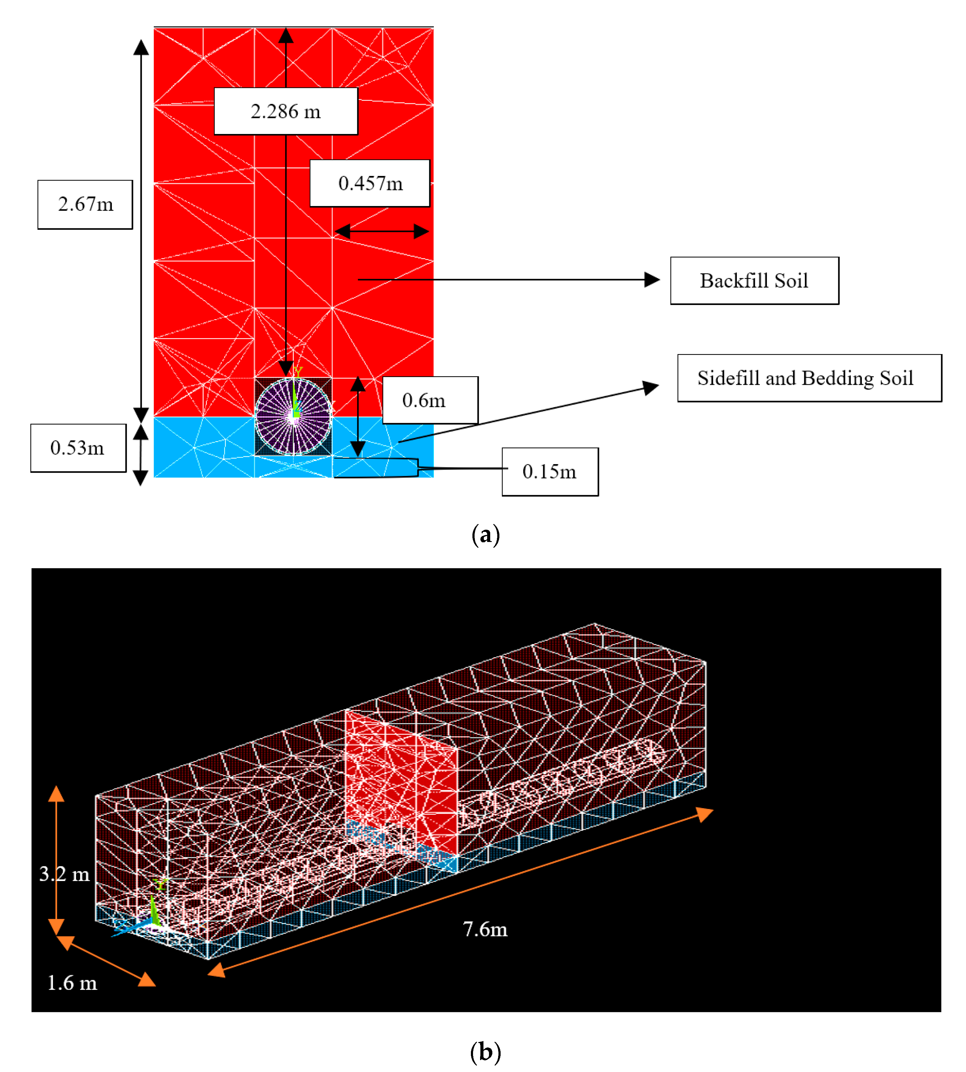
Figure 6.
Verification of tensile stress–strain behavior of current study and the previous study (Zamanian [28]) depending on different element types used for soil and concrete pipe.
Figure 6.
Verification of tensile stress–strain behavior of current study and the previous study (Zamanian [28]) depending on different element types used for soil and concrete pipe.
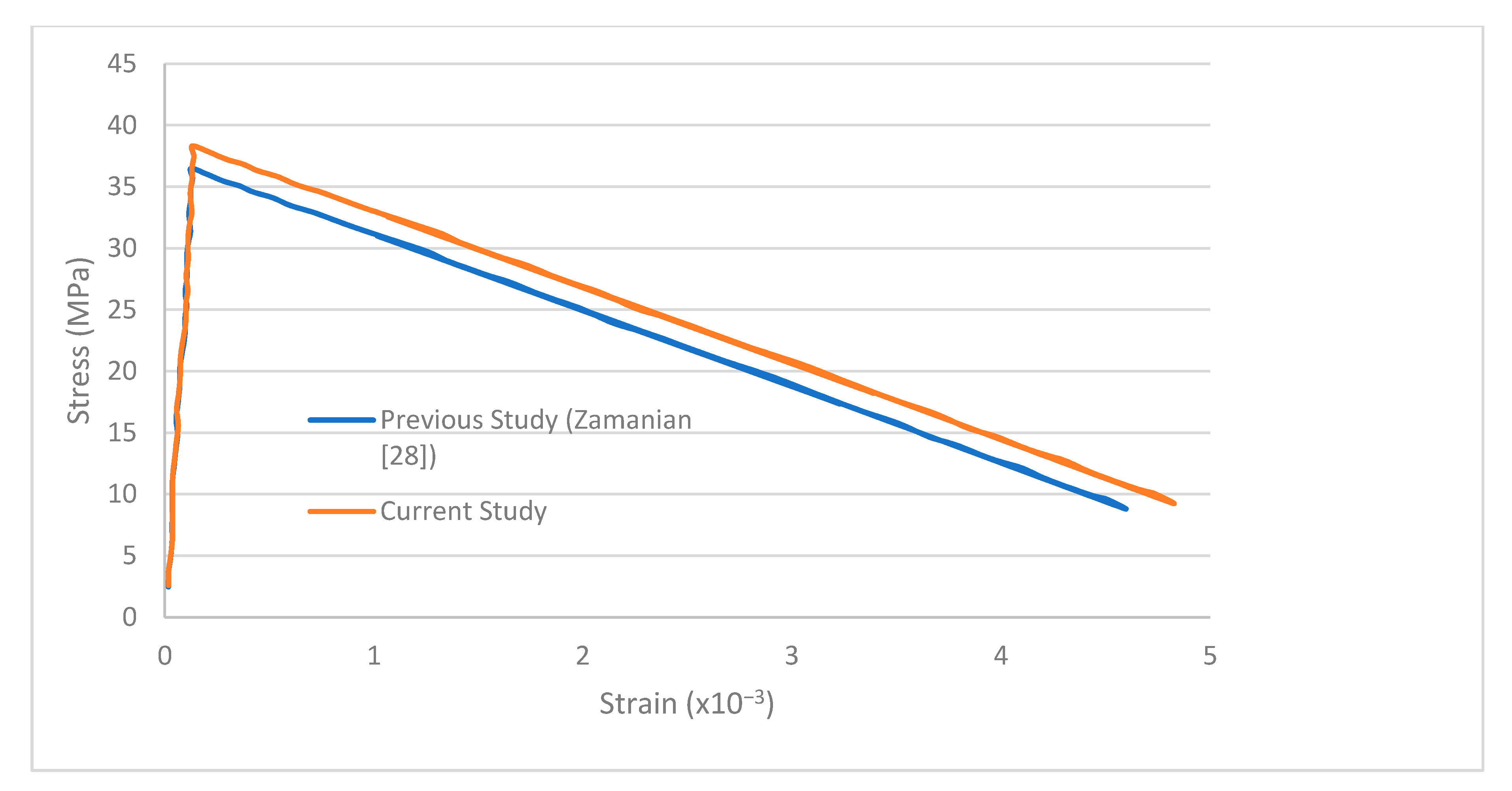
Figure 7.
The geometry of the calibrated unreinforced concrete sewer pipe in ANSYS in accordance with ASTM Specification C14–15 with reference to AASHTO.
Figure 7.
The geometry of the calibrated unreinforced concrete sewer pipe in ANSYS in accordance with ASTM Specification C14–15 with reference to AASHTO.

Figure 8.
Element type and geometry details of the GPC pipe model.
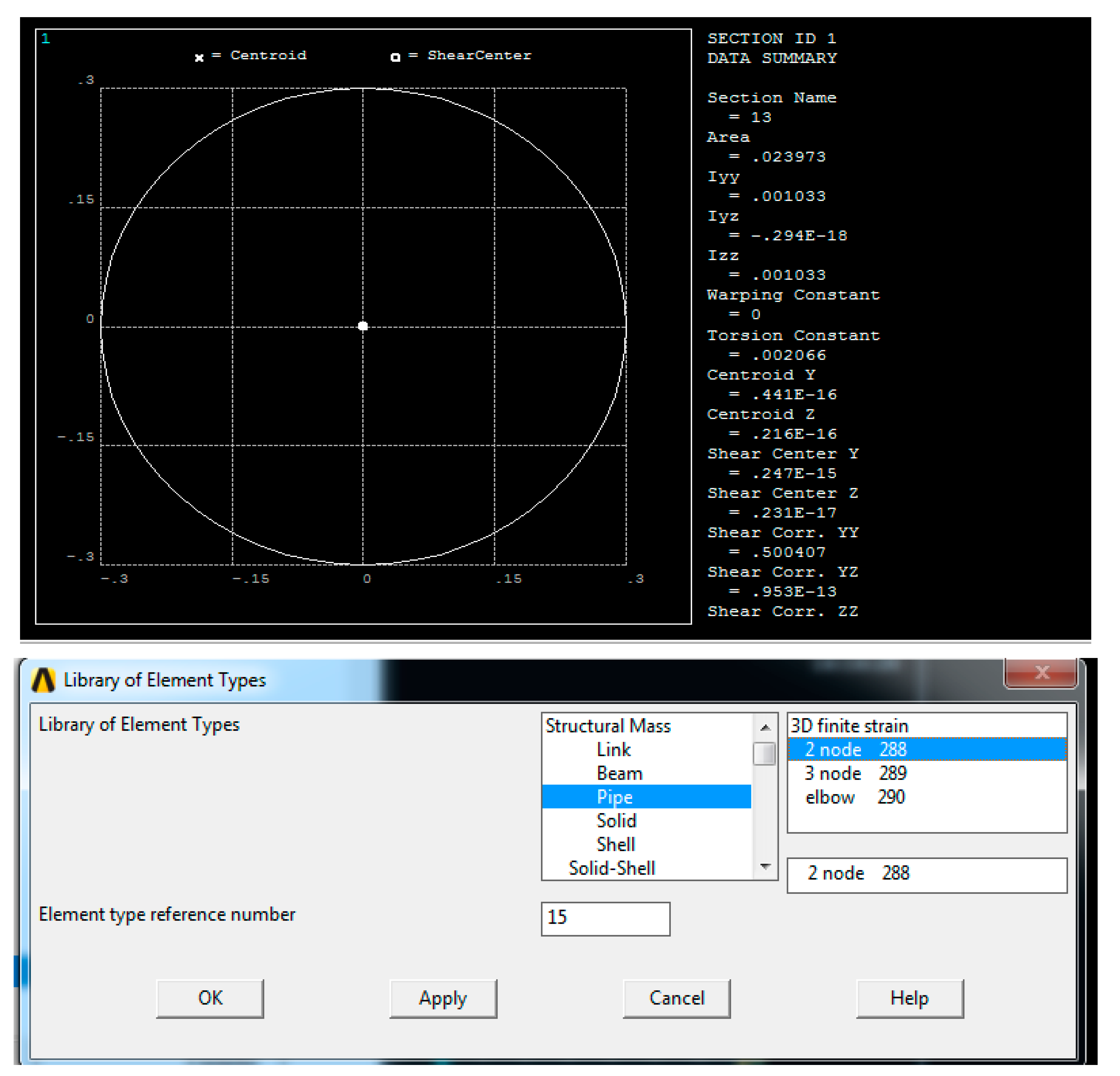
Figure 9.
The static loading applied in the middle part of the GPC pipe in ANSYS.
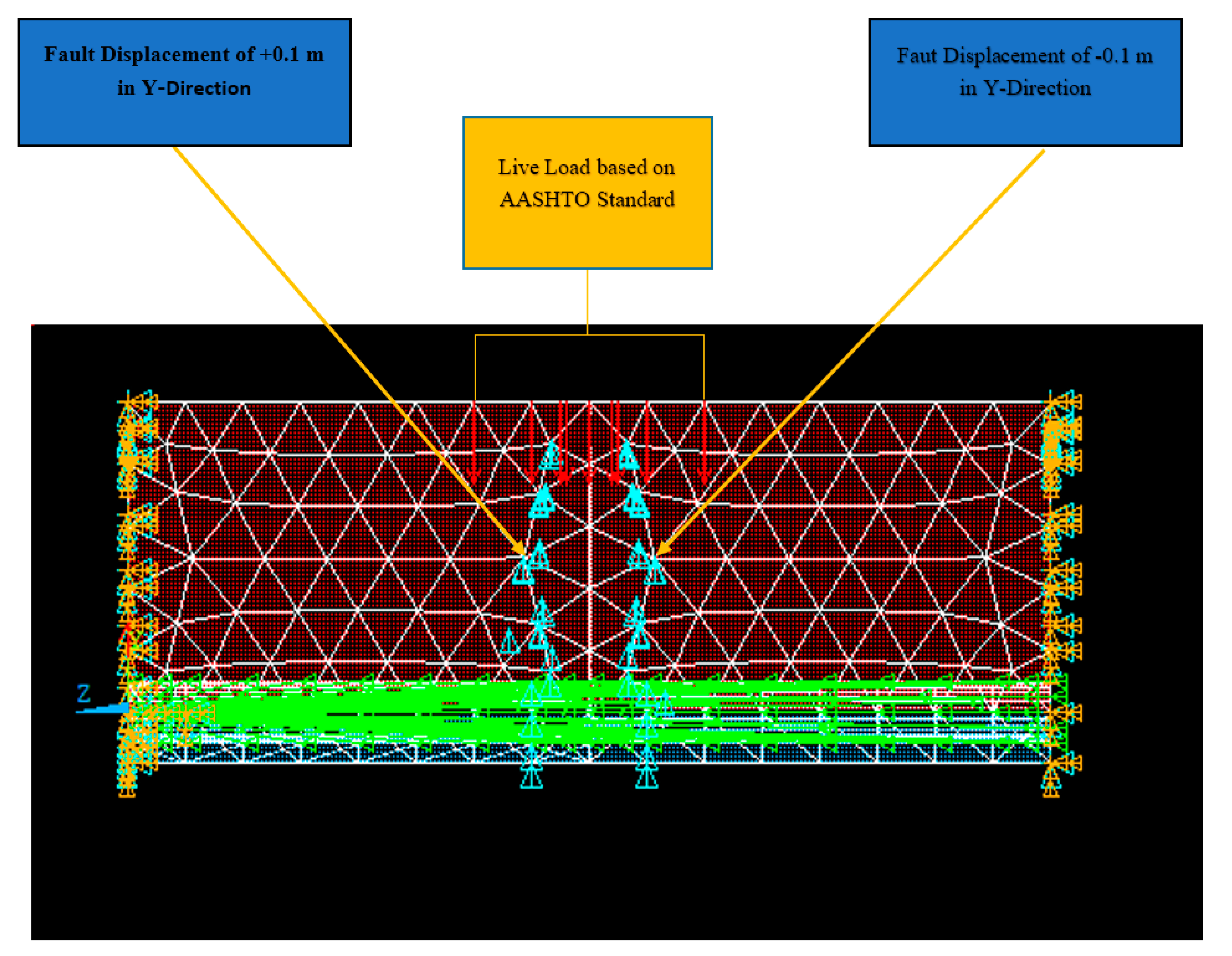
Figure 10.
The X-displacement series of the Tabas earthquake, Iran 1978 (Peer Ground Motion Database [43]).
Figure 10.
The X-displacement series of the Tabas earthquake, Iran 1978 (Peer Ground Motion Database [43]).
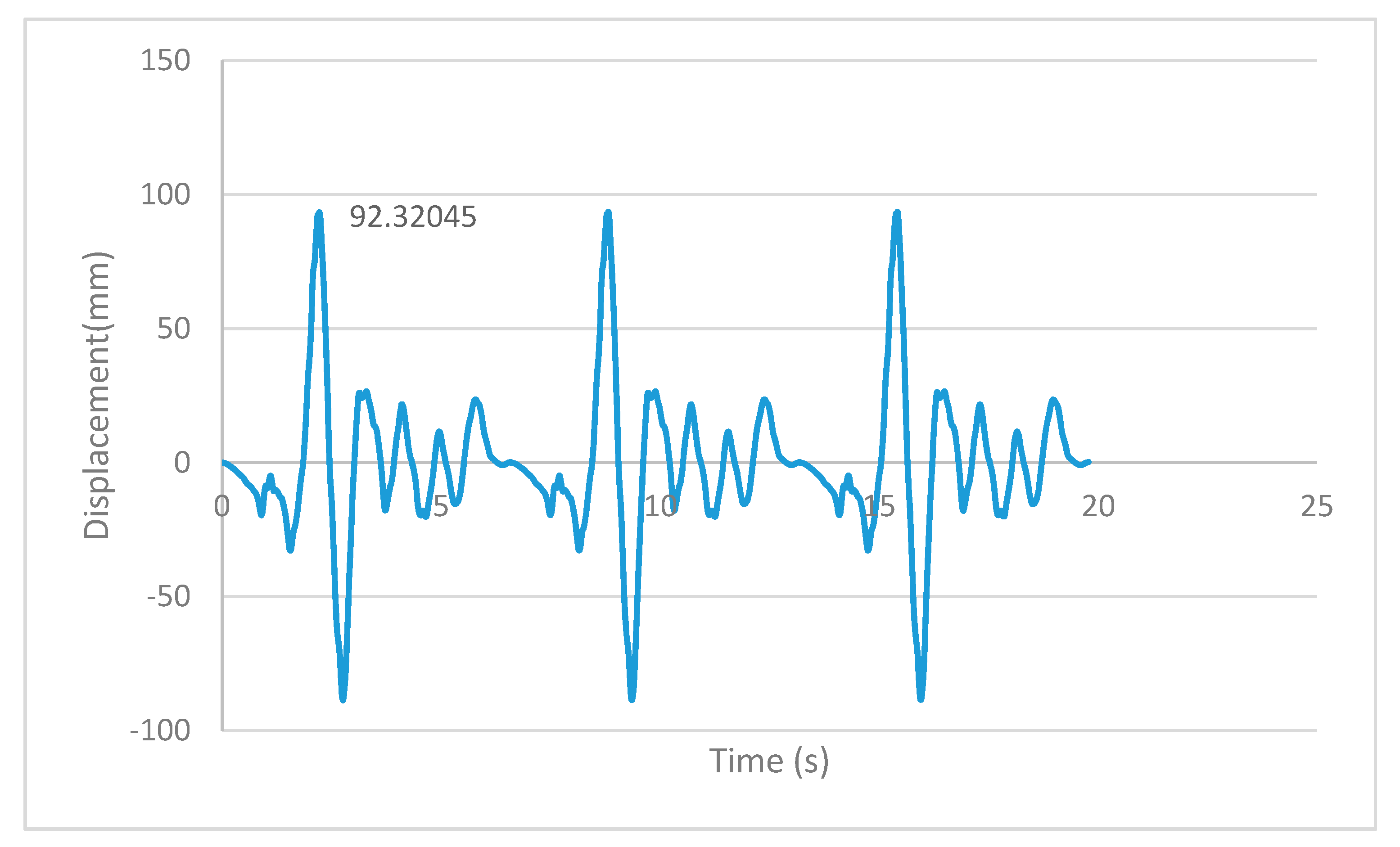
Figure 11.
The X-displacement series of the Friuli earthquake, Italy 1981 (Peer Ground Motion Database [43]).
Figure 11.
The X-displacement series of the Friuli earthquake, Italy 1981 (Peer Ground Motion Database [43]).

Figure 12.
The accelerogram of the Tabas earthquake, Iran 1978 (Peer Ground Motion Database [43]).
Figure 12.
The accelerogram of the Tabas earthquake, Iran 1978 (Peer Ground Motion Database [43]).

Figure 13.
The accelerogram of the Friuli earthquake, Italy 1981 (Peer Ground Motion Database [43]).
Figure 13.
The accelerogram of the Friuli earthquake, Italy 1981 (Peer Ground Motion Database [43]).

Figure 14.
Typical soil and GPC pipe settlements under static loads (a) isometric view (b) side view.
Figure 14.
Typical soil and GPC pipe settlements under static loads (a) isometric view (b) side view.

Figure 15.
Application of fixed-support on both sides of the FE model of soil–GPC pipe in ANSYS.

Figure 16.
The settlement of applied static loadings in (a) 2D and (b) 3D view.
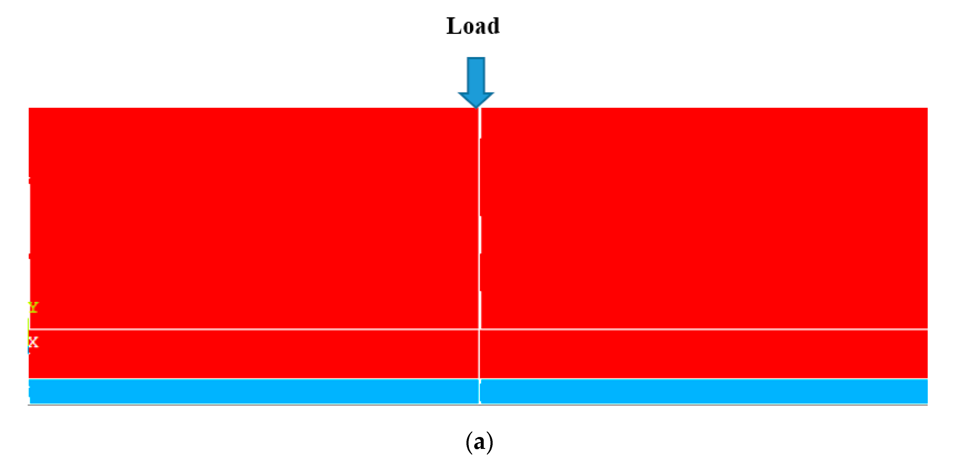
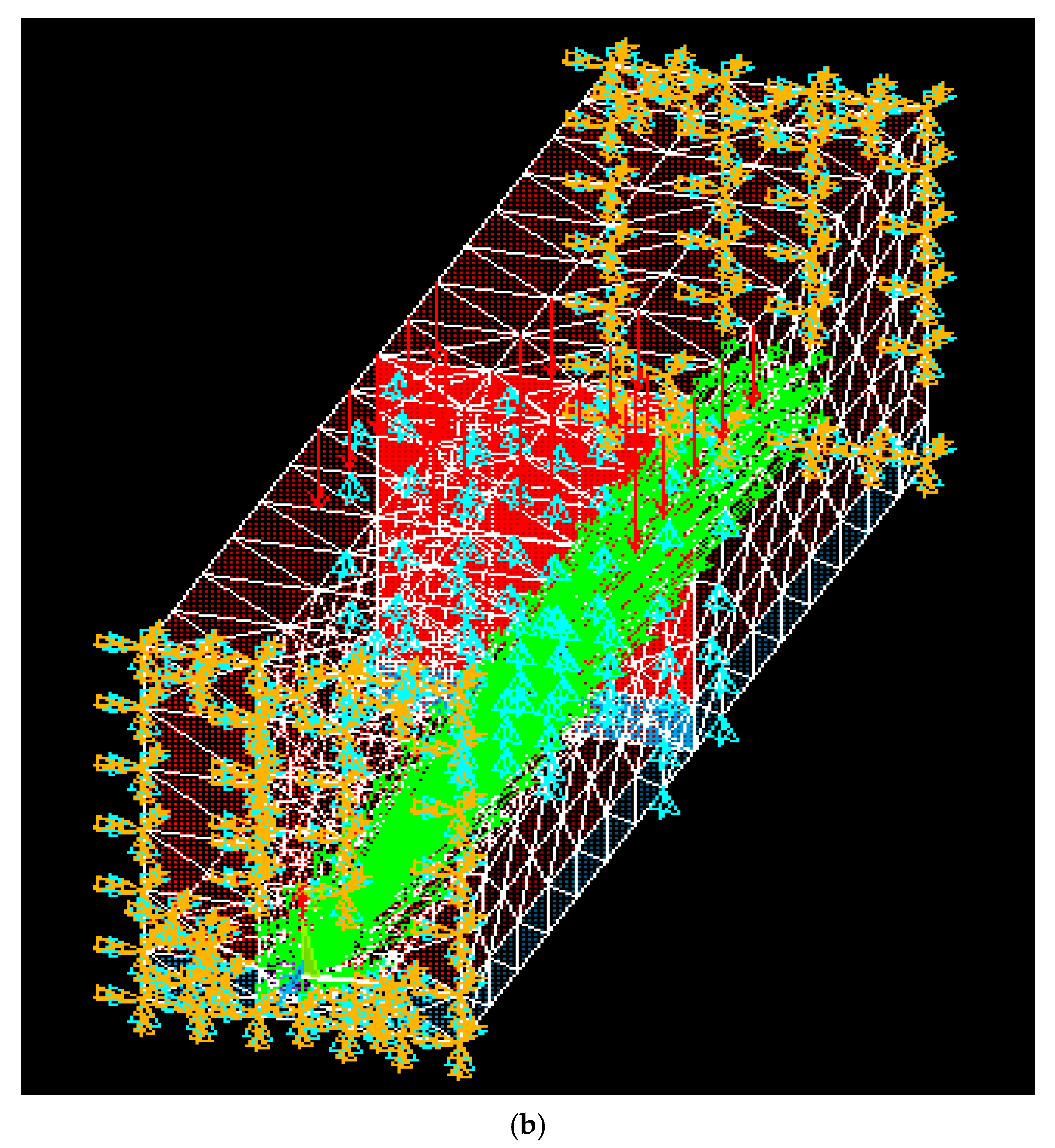
Figure 17.
The typical vertical displacement of the GPC pipe.
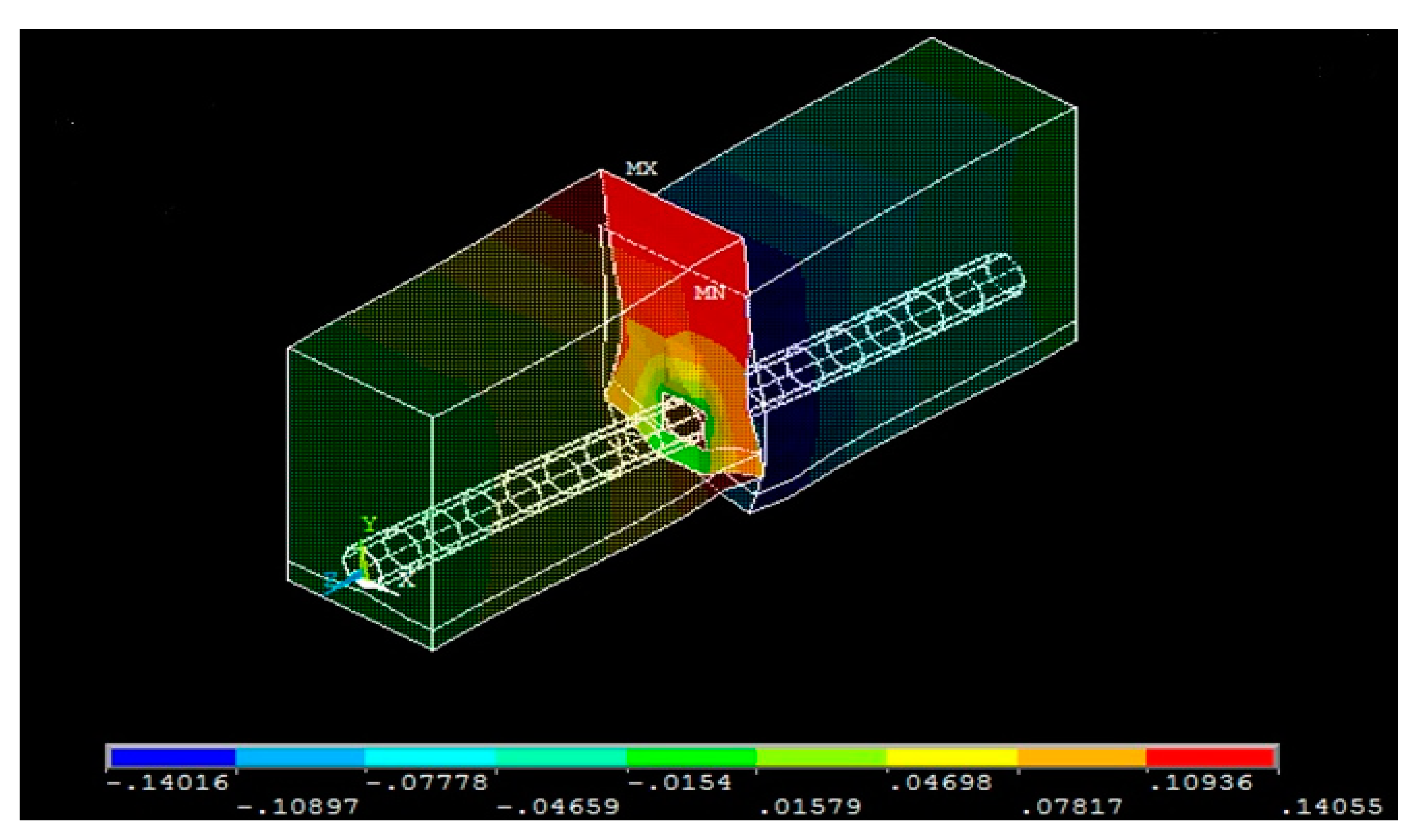
Figure 18.
Horizontal and vertical displacements at node 20, element 1126 with coordinate details: (x = 0, y = 0.25, z = −4) and 0% FA.
Figure 18.
Horizontal and vertical displacements at node 20, element 1126 with coordinate details: (x = 0, y = 0.25, z = −4) and 0% FA.

Figure 19.
Horizontal and vertical displacements at node 20, element 1126 with coordinate details: (x = 0, y = 0.25, z = −4) and 10% FA.
Figure 19.
Horizontal and vertical displacements at node 20, element 1126 with coordinate details: (x = 0, y = 0.25, z = −4) and 10% FA.
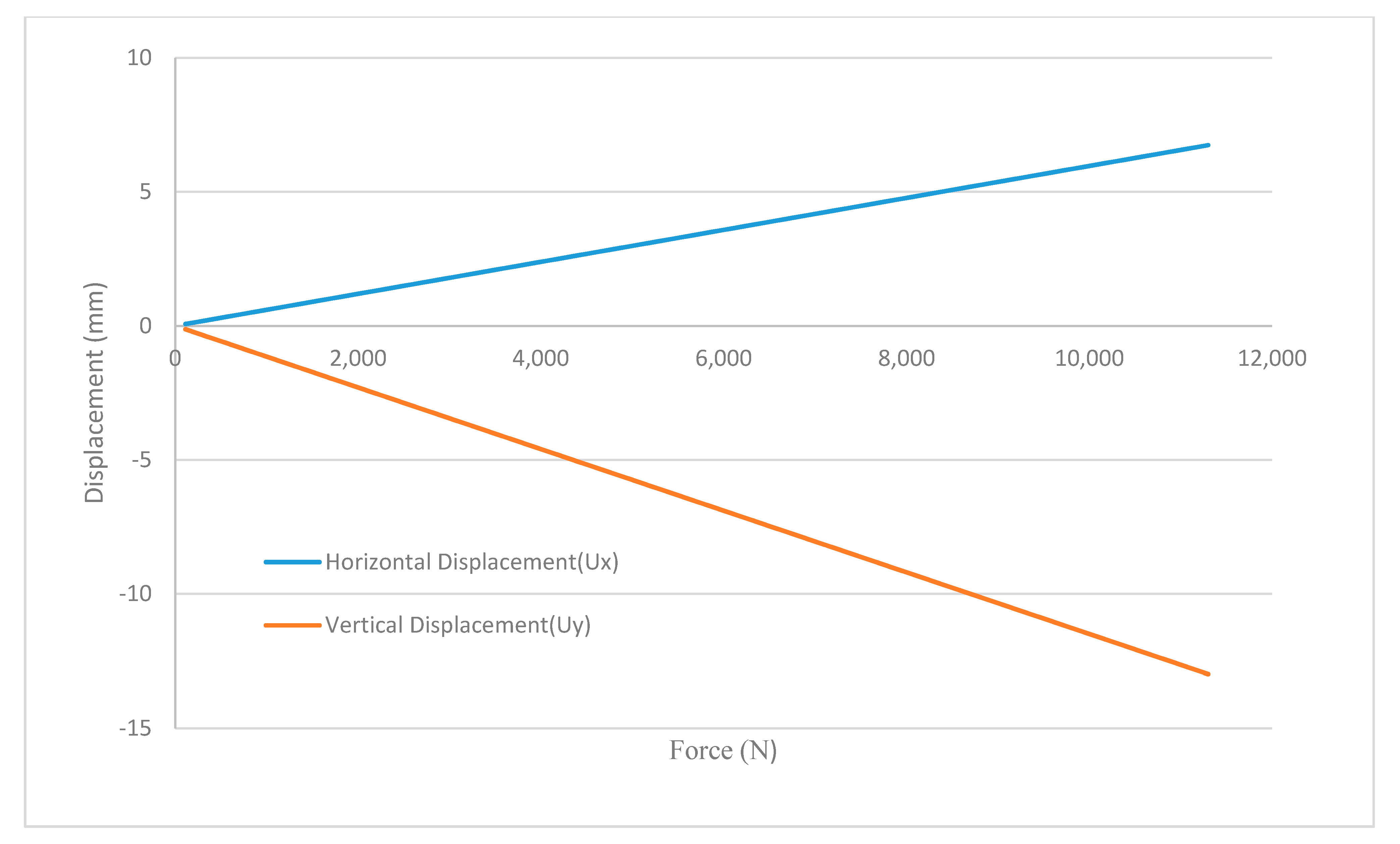
Figure 20.
Horizontal and vertical displacements at node 20, element 1126 with coordinate details: (x = 0, y = 0.25, z = −4) and 20% FA.
Figure 20.
Horizontal and vertical displacements at node 20, element 1126 with coordinate details: (x = 0, y = 0.25, z = −4) and 20% FA.

Figure 21.
Horizontal and vertical displacements at node 20, element 1126 with coordinate details: (x = 0, y = 0.25, z = −4) and 30% FA.
Figure 21.
Horizontal and vertical displacements at node 20, element 1126 with coordinate details: (x = 0, y = 0.25, z = −4) and 30% FA.

Figure 22.
Horizontal and vertical displacements at node 20, element 1126 with coordinate details: (x = 0, y = 0.25, z = −4) and 50% FA.
Figure 22.
Horizontal and vertical displacements at node 20, element 1126 with coordinate details: (x = 0, y = 0.25, z = −4) and 50% FA.

Figure 23.
Horizontal and vertical displacements at node 20, element 1126 with coordinate details: (x = 0, y = 0.25, z = −4) and 70% FA.
Figure 23.
Horizontal and vertical displacements at node 20, element 1126 with coordinate details: (x = 0, y = 0.25, z = −4) and 70% FA.

Figure 24.
Comparison of vertical and horizontal displacements at node 20, element 1126 among all GPC mixtures with 0%, 10%, 20%, 30%, 50%, 70% FA.
Figure 24.
Comparison of vertical and horizontal displacements at node 20, element 1126 among all GPC mixtures with 0%, 10%, 20%, 30%, 50%, 70% FA.
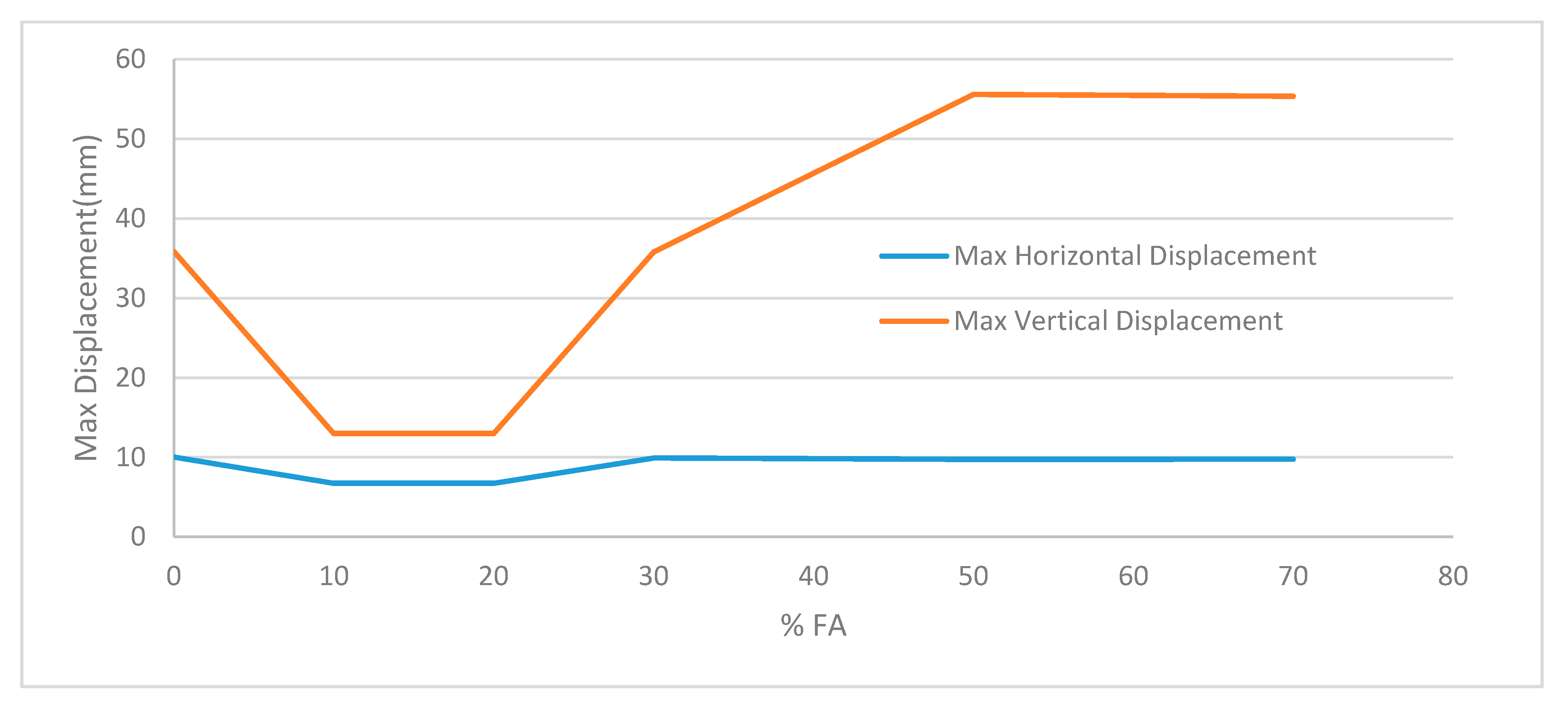
Figure 25.
Comparison of time-history curves for vertical displacement of the pipe crown with the inclusion of 20% and 0% FA due to the Tabas earthquake.
Figure 25.
Comparison of time-history curves for vertical displacement of the pipe crown with the inclusion of 20% and 0% FA due to the Tabas earthquake.
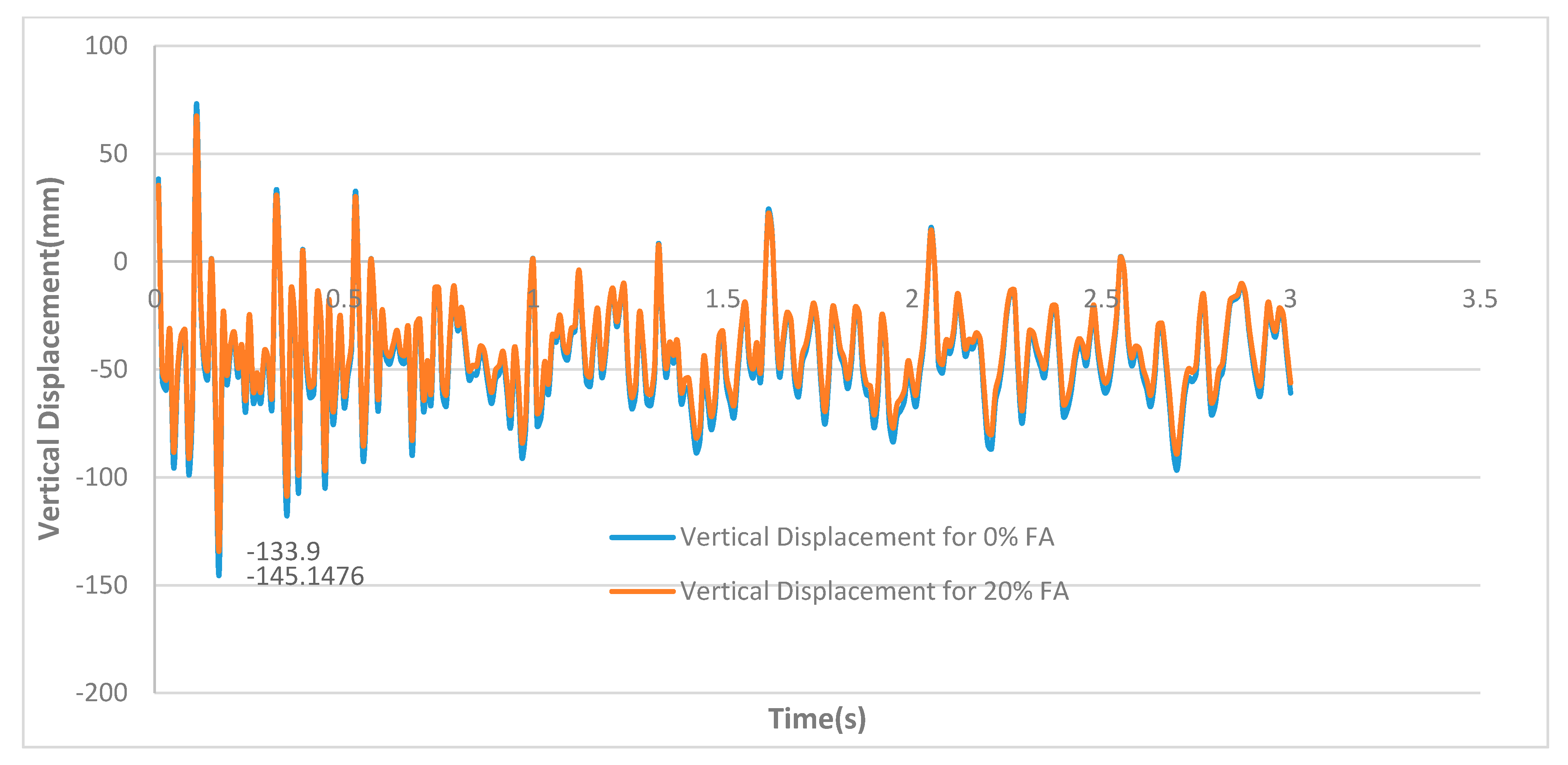
Figure 26.
Comparison of time-history curves for horizontal displacement of the pipe crown with the inclusion of 20% and 0% FA due to the Tabas earthquake.
Figure 26.
Comparison of time-history curves for horizontal displacement of the pipe crown with the inclusion of 20% and 0% FA due to the Tabas earthquake.
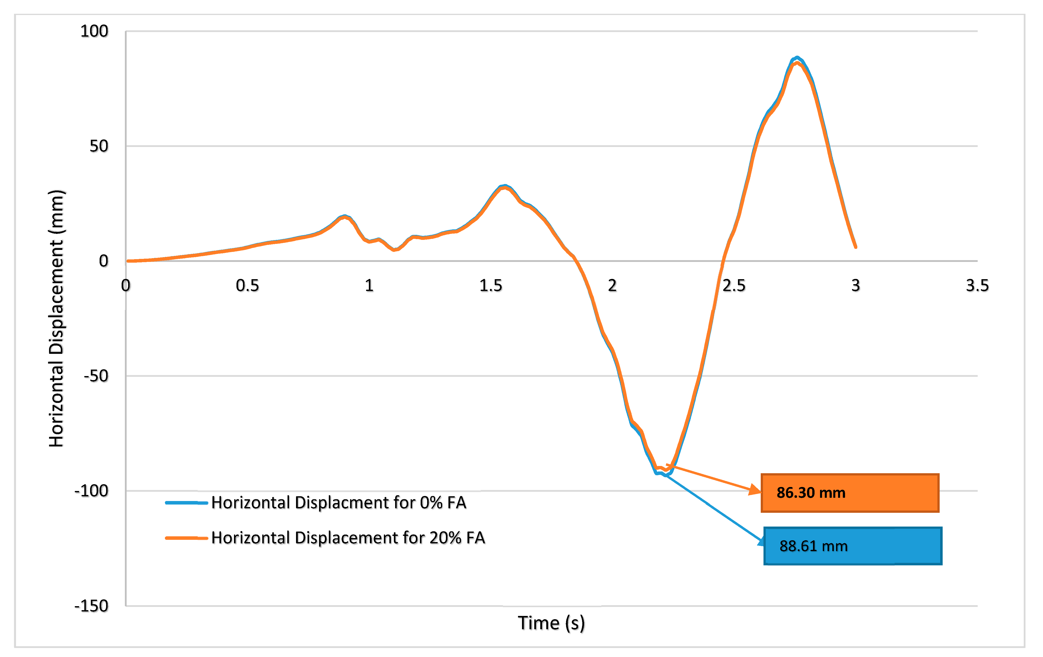
Figure 27.
The comparison of the reaction force of fixed-support in the time-history analysis under different FA dosages (a) 0% FA, (b) 20% FA.
Figure 27.
The comparison of the reaction force of fixed-support in the time-history analysis under different FA dosages (a) 0% FA, (b) 20% FA.

Figure 28.
Comparison of time-history curves for vertical displacement of the pipe crown with the inclusion of 20% and 0% FA due to the Friuli earthquake.
Figure 28.
Comparison of time-history curves for vertical displacement of the pipe crown with the inclusion of 20% and 0% FA due to the Friuli earthquake.

Figure 29.
Comparison of time-history curves for horizontal displacement of the pipe crown with the inclusion of 20% and 0% FA due to the Friuli earthquake.
Figure 29.
Comparison of time-history curves for horizontal displacement of the pipe crown with the inclusion of 20% and 0% FA due to the Friuli earthquake.
Table 2.
Concrete failure criteria constants in ANSYS (William–Warnke).
| ANSYS Parameters | Values |
|---|---|
| The shear transfer coefficient for open cracks (βt) | 0.3 |
| The shear transfer coefficient for closed cracks (βC) | 1 |
| Uniaxial cracking stress (fr) | 46.23 MPa |
| Uniaxial crushing stress (f′c) | 38 MPa |
| Biaxial compressive strength (fcb′) | 45.40 MPa |
| Ambient hydrostatic stress (σh) | 65.46 MPa |
| Hydrostatic biaxial crush stress (f1) | 54.86 MPa |
| Hydrostatic uniaxial crash stress (f2) | 65.08 MPa |
| Tensile Crack Factor | 0.6 |
| Elasticity modulus (E) | 22,000 MPa |
| Poisson Ratio | 0.2 |
Table 3.
Comparison of numerical results in the present study and the modified Popovics model.
| Concrete Cube | Ultimate Load (KN) | Compressive Strength (MPa) | Strain at Peak Stress |
|---|---|---|---|
| GPC | |||
| Modified Popovics model (Isojeh et al. [22]) | 851.4 | 37.84 | 0.002086 |
| ANSYS (Present Study) | 858.15 | 38.14 | 0.002262 |
Table 4.
Static loading proposed for the validation of numerical results.
| Static Loads | Gravity (Soil Weight) (N) | 9.81 |
| Traffic Loads (Pa) | 631,000 | |
| Internal sewage water pressure (Pa) | 276,000–414,000 |
Table 5.
Material properties of soil and concrete for validation in FE.
| Density | Total Static Loading | Element Type | ||||||||||
|---|---|---|---|---|---|---|---|---|---|---|---|---|
| Material Type | lb/In3 | Kg/m3 | Lbs | N | Concrete | Soil | Poisson Ratio (ν) | βt | βc | |||
| Concrete | 0.0868 | 2402 | 450,006 | 200,198 | Previous Study | Current Study | Previous Study | Current Study | Concrete | 0.2 | 0.3 | 1 |
| Sidefill & Bedding Soil | 0.0625 | 1730 | Solid 65 | Pipe 288 | Solid 65 | Solid 185 | Sidefill & Bedding Soil | 0.25 | N/A | N/A | ||
| Backfill Soil | 0.0734 | 2032 | Backfill Soil | 0.3 | N/A | N/A | ||||||
Table 6.
Material properties of soil and GPC pipe.
| Parameters Material Type | Elastic Properties | Plastic Properties | Element Type | Internal Friction Coefficient Soil-Pipe | |||
|---|---|---|---|---|---|---|---|
| GPC Concrete | Elasticity Modulus (GPa) | 15–22 | βt | 0.2 | Pipe 288 | 0.6–0.7 | |
| βc | 0.8 | ||||||
| Poisson Ratio (ν) | 0.25 | Tensile Crack Factor | 0.6 | ||||
| Density (Kg/m3) | 2420 | ||||||
| Soil | Sidefill & Bedding (Cohesive) | Elasticity Modulus (GPa) | 0.019 | Cohesive Strength (C-Kpa) | 17–252 | Solid 185 | |
| Poisson Ratio (ν) | 0.25 | Friction Angle (φ) | 20–29 | ||||
| Density (Kg/m3) | 1730 | Dilation angle (Ψ) | 2 | ||||
| Backfill (Sandy) | Elasticity Modulus (GPa) | 0.028 | Cohesive Strength (C-Kpa) | 0–17 | |||
| Poisson Ratio (ν) | 0.3 | Friction Angle (φ) | 35–40 | ||||
| Density (Kg/m3) | 2032 | Dilation angle (Ψ) | 2 | ||||
Table 7.
Pipe geometry in ANSYS.
| Pipe Geometry | In | M |
|---|---|---|
| Internal Diameter | 24 | 0.6 |
| Wall Thickness | 3 | 0.076 |
| Pipe Length | 300 | 7.6 |
Table 8.
Standard installation soil and minimum compaction requirements (ASCE 15-98).
| Installation Type | Bedding Thickness | Haunch and Outer Bedding | Lower Side |
|---|---|---|---|
| Type 1 | minimum, not less than 150 mm | 95% Category I | 90% Category I, 95% Category II, Or 100% Category III |
| Type 2 | minimum, not less than 150 mm | 90% Category I Or 95% Category II | 85% Category I, 90% Category II, Or 95% Category III |
| Type 3 | minimum, not less than 150 mm | 85% Category I, 90% Category II, Or 95% Category III | 85% Category I, 90% Category II, Or 95% Category III |
| Type 4 | minimum, not less than 150 mm | No Compaction is required, except if Category III, Use 85% | No Compaction is required, except if Category III, Use 85% |
Table 9.
The values of the seismic and static loadings applied in FE.
| Static Loads | Gravity (Soil weight) N | 9.81 |
| Traffic loads (Pa) | 74,137 | |
| Internal sewage water pressure in the pipe | 276,000–414,000 Pa | |
| Fault displacement in the middle part of GPC pipe | 0.1 m | |
| Seismic Loads (1) (Tabas (Iran), 1978) | Peak displacement of TABAS earthquake (m) | 0.093 m |
| History time (s) | 19.78 (s) | |
| Seismic Loads (2) (Friuli (Italy), 1981) | Peak displacement of Friuli earthquake (m) | 0.025 m |
| History time (s) | 15.175 (s) |
Table 10.
Material number defined for meshing in ANSYS.
| Material Type | No. | Density (Kg/m3) |
|---|---|---|
| GPC concrete | 1 | 2420 |
| Internal fluid (Sewage) | 2 | 706 |
| Backfill (Soil type 1) | 3 | 2032 |
| Sidefill and Bedding (Soil type 2) | 4 | 1730 |
Table 11.
Compressive strength of various mixes without alkaline solution (AS).
| Mix | % FA | Compressive Strength (MPa) | Curing Conditions | |
|---|---|---|---|---|
| 7 Days | 28 Days | Water Bath at 21 °C | ||
| PF10000 | 0 | 21.56 | 31.93 | Water Bath at 21 °C |
| PF9010B | 10 | 24.99 | 36.63 | Water Bath at 21 °C |
| PF8020 | 20 | 25.24 | 37.84 | Water Bath at 21 °C |
| PF7030C | 30 | 18.44 | 31.03 | Water Bath at 21 °C |
| PF5050A | 50 | 11.68 | 24.53 | Water Bath at 21 °C |
| PF3070A | 70 | 5.49 | 12.33 | Water Bath at 21 °C |
Table 12.
The details of concrete mixtures with different ratios of AS for dosages of 30%, 50%, 70% FA.
Table 12.
The details of concrete mixtures with different ratios of AS for dosages of 30%, 50%, 70% FA.
| Mix | % FA | NaOH (gr) | Na2SiO3 (gr) | Water (mL) | Na2SiO3/ NaOH | NaOH Molarity (M) | AS/FA |
|---|---|---|---|---|---|---|---|
| PF7030A | 30 | 250 | 625 | 1500 | 2.5 | 4.16 | 0.25 |
| PF7030B | 30 | 250 | 625 | 1500 | 2.5 | 4.16 | 0.25 |
| PF5050B | 50 | 428 | 1070 | 1500 | 2.5 | 7.13 | 0.25 |
| PF3070B | 70 | 600 | 1500 | 1500 | 2.5 | 10 | 0.25 |
Table 13.
Compressive strength of various mixes with AS for the percentages of 30%, 50%, 70% FA.
| Mix | % T2PC | % FA | Average Compressive Strength (MPa) | Curing Condition | |
|---|---|---|---|---|---|
| 7 Days | 28 Days | ||||
| PF7030B | 70 | 30 | 8.14 | 14.58 | Water bath at 21 °C |
| PF5050B | 50 | 50 | 5.97 | 10.55 | Water bath at 21 °C |
| PF3070B | 30 | 70 | 10.02 | 15.63 | Water bath at 21°C |
Table 14.
Material properties for nonlinear concrete in ANSYS calculated based on experimental results of the present study.
Table 14.
Material properties for nonlinear concrete in ANSYS calculated based on experimental results of the present study.
| ANSYS Parameters | Values |
|---|---|
| The shear transfer coefficient for open cracks (βt) | 0.2 |
| The shear transfer coefficient for closed cracks (βC) | 0.8 |
| Uniaxial cracking stress (fr) | 46.13 |
| Uniaxial crushing stress (f′c) | 37.84 |
| Biaxial compressive strength (fcb′) | 45.408 |
| Ambient hydrostatic stress (σh) | 65.46 |
| Hydrostatic biaxial crush stress (f1) | 54.86 |
| Hydrostatic uniaxial crush stress (f2) | 65.08 |
| Elasticity modulus (E) | 22,000 |
Publisher’s Note: MDPI stays neutral with regard to jurisdictional claims in published maps and institutional affiliations. |
© 2021 by the authors. Licensee MDPI, Basel, Switzerland. This article is an open access article distributed under the terms and conditions of the Creative Commons Attribution (CC BY) license (https://creativecommons.org/licenses/by/4.0/).
Share and Cite
MDPI and ACS Style
Mostofizadeh, S.; Tee, K.F. Static and Seismic Responses of Eco-Friendly Buried Concrete Pipes with Various Dosages of Fly Ash. Appl. Sci. 2021, 11, 11700. https://doi.org/10.3390/app112411700
AMA Style
Mostofizadeh S, Tee KF. Static and Seismic Responses of Eco-Friendly Buried Concrete Pipes with Various Dosages of Fly Ash. Applied Sciences. 2021; 11(24):11700. https://doi.org/10.3390/app112411700
Chicago/Turabian StyleMostofizadeh, Sayedali, and Kong Fah Tee. 2021. "Static and Seismic Responses of Eco-Friendly Buried Concrete Pipes with Various Dosages of Fly Ash" Applied Sciences 11, no. 24: 11700. https://doi.org/10.3390/app112411700
Note that from the first issue of 2016, this journal uses article numbers instead of page numbers. See further details here.