A Simple Model of Ballistic Conduction in Multi-Lead Molecular Devices

Abstract

A fully analytical model is presented for ballistic conduction in a multi-lead device that is based on a $\pi$-conjugated carbon framework attached to a single source lead and several sink leads. This source-and-multiple-sink potential (SMSP) model is rooted in the Ernzerhof source-and-sink potential (SSP) approach and specifies transmission in terms of combinations of structural polynomials based on the molecular graph. The simplicity of the model allows insight into many-lead devices in terms of constituent two-lead devices, description of conduction in the multi-lead device in terms of structural polynomials, molecular orbital channels, and selection rules for active and inert leads and orbitals. In the wide-band limit, transmission can be expressed entirely in terms of characteristic polynomials of vertex-deleted graphs. As limiting cases of maximum connection, complete symmetric devices (CSD) and complete bipartite symmetric devices (CBSD) are defined and solved analytically. These devices have vanishing lead-lead interference effects. Illustrative calculations of transmission curves for model small-molecule systems are presented and selection rules are identified.

1. Introduction

The study of molecular conduction and molecule-scale devices is and has been an active area at the boundary between chemistry and physics for at least half a century [1], and by now, it has accumulated a substantial number of textbooks in the literature, e.g., [2,3,4,5,6]. Over this period, different theoretical approaches have emerged. Techniques for calculation have mainly favoured Green’s Function (GF) methods, both equilibrium and non-equilibrium GFs [7,8,9,10,11,12,13,14,15,16,17,18,19]. Especially in chemistry, there has been a sustained development of scattering models for the ballistic conduction of electrons though molecular systems, with an emphasis on conduction through channels governed by energies and symmetry characteristics of orbitals [20,21,22,23,24,25,26,27,28,29,30]. An advantage of such pictures is that they lend themselves to even simpler qualitative modelling of the effects of electron energy, relative interaction strengths, contact placement, and qualitative features of molecular electronic structures, as treated in e.g., [31,32,33,34] and as illustrated by many examples in our own work, as cited below.

One successful model of this type is the Source-and-Sink-potential (SSP) model proposed and developed by Ernzerhof and co-workers in tandem with their DFT approach to an a priori calculation of conduction [35,36,37,38,39,40,41,42,43,44,45,46,47,48,49,50,51,52,53,54]. The SSP approach replaces the doubly infinite system of molecule and leads by the finite system of a molecule dressed with a source and a sink pseudo atom equipped with complex potentials, hence in the tight-binding model replacing an $(n+\infty )\times (n+\infty )$ matrix problem by an $(n+2)\times (n+2)$ problem [40,55]. These ideas have their roots in earlier work [56,57] and have parallels in approaches such as SSM [58] and CAP [59].

A special feature of the SSP model in its graph theoretical incarnation [55] is that it gives a useful qualitative account of the two-lead device, giving selection rules for conduction, rationalisation of the sensitivity of current to placing of leads; models for composite devices; and a general classification of types of conduction behaviour, such as equiconduction, omniconduction, omni-insulation, and perfect reflection [60,61,62,63,64,65,66,67,68,69]. Although the graph theoretical version of SSP is based on the Hückel (tight-binding) model of electronic structure, many of its most useful features persist at higher levels of theory. Conduction of the Hückel device can be analysed in terms of internal channels based on molecular orbitals of the central molecule, which are either active or inert [63]. It can be shown [70] that, as the level of theory is raised, a similar analysis applies to Hartree–Fock MO channels and, then at the second-order (or higher) Green’s Function level, to internal channels associated with Dyson orbitals. This evolution of the channel picture is consistent with the standard Meir–Wingreen [19] and Landauer–Büttiker [71,72] expressions for elastic conduction of electrons through molecules.

Green’s Function approaches have been applied to various multi-lead configurations at various levels of theory. For instance, Reference [59] quotes a dozen examples, and public domain codes such as TRANSIESTA [73] allow for calculations with many leads. Explicit high-level calculations of transmission for individual systems are undoubtedly valuable, but there is still a role for simple models that can identify broad trends for families of systems, can give a framework for interpretation, and can identify cases for more detailed analysis by a priori/ab initio methods.

In line with this philosophy, our aim in the present paper is to generalise the two-lead SSP formalism to deal with multi-lead devices, retaining its many advantages. To be concrete, we call this version of SSP the SMSP (source-and-multiple-sink-potential) model. The paradigm system for this model has a single-source lead connected to one atom of the central molecule, and several drain leads attached to other specific atoms. Ernzerhof already considered an extension of SSP with a three-lead device that has a gating arrangement that includes two sources and one sink [51]. We defer treatment of the many possible multi-source variations of SMSP to future work.

As with SSP, we are able to obtain an analytical solution at the Hückel/Tight-Binding level for non-trivial molecular systems in terms of a set of characteristic polynomials. General expressions for the currents in all the leads can be developed and used to identify global selection rules. They suggest new classes of conductors, by analogy with developments in the theory for the original two-lead device. The model shares with SSP the same opportunities for seamless transition from Hückel to self-consistent and correlated treatments.

The structure of the paper is as follows: Section 2 describes the basic SSP model; Section 3 introduces the SMSP model equations, their formal solution and simplification for devices with symmetric (i.e., chemically identical) leads, and the analysis of molecular orbital conduction channels and lead-lead interference effects; Section 4 treats two classes of ‘complete’ devices, in which either all vertices of the molecular graph (CSD) or all vertices of a given partite set (CBSD) are connected to leads and which turn out to have minimal interference effects; Section 5 shows how to break down conduction into contributions from internal molecular channels; Section 6 reports illustrative results, Section 7 outlines the connections of the present model with the Meir–Wingreen approach; and Section 8 reports our main conclusions.

2. Two-Lead Devices

In the standard two-lead SSP model, the device consists of a central molecule that is attached by single-atom contacts to the leads (Figure 1). In the steady state, the source lead supports an incoming electron wave that undergoes partial reflection at the interface with the molecule, and the transmitted part of the wave scatters through the molecule and exits into the sink lead. The essential observation behind the model [40] is that the two semi-infinite leads may be replaced by source and sink pseudo-atoms equipped with appropriate complex potentials, which play the roles of delivering the transmitted fraction of the electron to the molecule and removing it downstream, respectively. In the purely graph theoretical version of the model, this step allows replacement of a doubly infinite system by one in which the $n\times n$ Hermitian (in fact, real symmetric) molecular Hamiltonian matrix is expanded to an $(n+2)\times (n+2)$ non-Hermitian matrix. It is convenient to recast this generalised eigenvalue problem in the form of an inhomogeneous linear equation [63]:

$$\mathbf{P}\mathbf{c}=\mathbf{b},$$

(1)

where $\mathbf{P}$ is the SSP matrix, the solution vector $\mathbf{c}$ gives the device wavefunction specified by complex entries on the $n+2$ vertices, and $\mathbf{b}$ is the inhomogeneity term that embodies the boundary conditions. The solution to this equation for each possible value of the energy of the incoming electron yields a compact expression for the zero-voltage transmission as a function of energy, $T\left(E\right)$, and as a bonus, gives a useful analysis of current in terms of bond or molecular-orbital (MO) contributions.

The transmission function can be cast in terms of the characteristic polynomials of four graphs, G, $G-\overline{\mathrm{L}}$, $G-\overline{\mathrm{R}}$, and $G-\overline{\mathrm{L}}-\overline{\mathrm{R}}$, where $\overline{\mathrm{L}}$ and $\overline{\mathrm{R}}$ are the centres within the graph that are in direct contact with the leads. These polynomials are denoted s, t, u, and v in [55]. Details of the algebra are given in the reference, but the result is that the device transmission has the form [63]:

$$T\left(E\right)=\mathcal{B}(q_{\mathrm{L}},q_{\mathrm{R}})\frac{j^2}{{\left|D\right|}^2},$$

(2)

where

$$\mathcal{B}(q_{\mathrm{L}},q_{\mathrm{R}})=(2{\beta }_{\mathrm{L}}sin{q}_{\mathrm{L}})(2{\beta }_{\mathrm{R}}sin{q}_{\mathrm{R}}){\beta }_{\mathrm{L}\mathrm{M}}^2{\beta }_{\mathrm{R}\mathrm{M}}^2$$

(3)

is a band-pass function ensuring that the electron energy is within the conduction bands of the leads, and the denominator is

$$D\left(E\right)={\beta }_{\mathrm{L}}{e}^{-i{q}_{\mathrm{L}}}{\beta }_{\mathrm{R}}{e}^{-i{q}_{\mathrm{R}}}s-{\beta }_{\mathrm{R}}{e}^{-i{q}_{\mathrm{R}}}{\beta }_{\mathrm{L}\mathrm{M}}^{2}t-{\beta }_{\mathrm{L}}{e}^{-i{q}_{\mathrm{L}}}{\beta }_{\mathrm{R}\mathrm{M}}^{2}u+{\beta }_{\mathrm{L}\mathrm{M}}^2{\beta }_{\mathrm{R}\mathrm{M}}^{2}v,$$

(4)

where the polynomials s, t, u, and v are to be defined below in (7), The incoming and outgoing wavevectors $q_{\mathrm{L}}$ and $q_{\mathrm{R}}$ satisfy the Hückel dispersion relations for the leads:

$$E={\alpha }_{\mathrm{L}}+2{\beta }_{\mathrm{L}}cos{q}_{\mathrm{L}}={\alpha }_{\mathrm{R}}+2{\beta }_{\mathrm{R}}cos{q}_{\mathrm{R}},$$

(5)

and we take the symmetric case where ${\alpha }_{\mathrm{L}}={\alpha }_{\mathrm{R}}=\alpha$, and ${\beta }_{\mathrm{L}}={\beta }_{\mathrm{R}}$, and refer the zero of all energies to $\alpha$. The polynomial $j^2$ satisfies [74]:

$$j^2=ut-sv,$$

(6)

where the four structural polynomials (SPs), s, t, u, and v, which are each the characteristic polynomial of a graph, are defined with respect to the characteristic matrix $E\mathbf{1}-\mathbf{A}$, where $\mathbf{A}$ is the adjacency matrix of the molecular graph:

$$\begin{array}{c}s=det\left(E\mathbf{1}-\mathbf{A}\right),\hfill \\ t=det{\left(E\mathbf{1}-\mathbf{A}\right)}^{\left[\overline{\mathrm{L}},\overline{\mathrm{L}}\right]},\hfill \\ u=det{\left(E\mathbf{1}-\mathbf{A}\right)}^{\left[\overline{\mathrm{R}},\overline{\mathrm{R}}\right]},\hfill \\ v=det{\left(E\mathbf{1}-\mathbf{A}\right)}^{\left[\overline{\mathrm{L}}\overline{\mathrm{R}},\overline{\mathrm{L}}\overline{\mathrm{R}}\right]},\hfill \end{array}$$

(7)

and j can be calculated directly [55,74] as

$$\begin{array}{cc}\hfill j& ={(-1)}^{\overline{\mathrm{L}}+\overline{\mathrm{R}}}det{\left(E\mathbf{1}-\mathbf{A}\right)}^{\left[\overline{\mathrm{L}},\overline{\mathrm{R}}\right]}.\hfill \end{array}$$

(8)

In these equations, superscripts indicate the sets of rows and columns to be deleted from the characteristic matrix.

The transmission $T\left(E\right)$ is therefore a ratio of polynomial functions of E, taking values between zero and one and depending implicitly on the molecular graph and the placement of connections. Questions such as transparency, opacity, selection rules, and linkage of transmission to MO channels can all be explored either analytically or numerically using this function [55,60,61,62,63,64,65,66,67,68,69].

In going to the more general device with multiple leads, the conceptual framework remains intact (Section 3), but the notation needs to be overhauled. The first point of difference concerns the naming of leads. We replace the $\mathrm{L}$ and $\mathrm{R}$ nomenclature for leads with numerical labelling. For the construction of derivations and proofs, it is convenient to adopt the convention that the source is lead 1, and the sink leads have labels $\mathrm{p}=2$ to l ($l\le n$). Centres in the molecule are then numbered 1 to n such that, for the first l centres, $\mathrm{p}$ in the molecule is connected to lead $\mathrm{p}$, and the numbers $l+1$ to n are then used for any centres that are not connected to leads. Formulas for transmission use this convention so that $T_{1\to \mathrm{M}}$ describes the transmission from the source to the molecule and $T_{\mathrm{M}\to \mathrm{p}}$ is the transmission from the molecule to sink lead, $\mathrm{p}$. Contiguous numbering of this type is advantageous for proofs that use the block structure of the characteristic matrix of bipartite molecular graphs, for example. (In this paper, we consider only devices where all leads are connected to distinct vertices of the molecular graphs. Degenerate ‘ipso’ [60] devices would need a modified numbering convention.)

A second adjustment is to the nomenclature for SPs. For larger numbers of leads, the labelling of every SP with a different letter becomes unwieldy, so we adopt a single symbol that can be extended to arbitrarily large cases. It is convenient to define

$$\begin{array}{c}{k}_{\mathrm{p},\mathrm{q}}={\beta }_{\mathrm{L}{\mathrm{M}}_{\mathrm{p}}}\mathrm{cof}{\left(E\mathbf{1}-\mathbf{A}\right)}_{\mathrm{p},\mathrm{q}}{\beta }_{\mathrm{L}{\mathrm{M}}_{\mathrm{q}}},\\ k_{\mathrm{p}\mathrm{q},\mathrm{r}\mathrm{s}}={\beta }_{\mathrm{L}{\mathrm{M}}_{\mathrm{p}}}{\beta }_{\mathrm{L}{\mathrm{M}}_{\mathrm{q}}}\mathrm{cof}{\left(E\mathbf{1}-\mathbf{A}\right)}_{\mathrm{p}\mathrm{q},\mathrm{r}\mathrm{s}}{\beta }_{\mathrm{L}{\mathrm{M}}_{\mathrm{r}}}{\beta }_{\mathrm{L}{\mathrm{M}}_{\mathrm{s}}},\\ \hfill k_{\mathrm{p}\mathrm{q}\cdots \mathrm{r},\mathrm{s}\mathrm{t}\cdots \mathrm{u}}={\beta }_{\mathrm{L}{\mathrm{M}}_{\mathrm{p}}}{\beta }_{\mathrm{L}{\mathrm{M}}_{\mathrm{q}}}\cdots {\beta }_{\mathrm{L}{\mathrm{M}}_{\mathrm{r}}}\mathrm{cof}{\left(E\mathbf{1}-\mathbf{A}\right)}_{\mathrm{p}\mathrm{q}\cdots \mathrm{r},\mathrm{s}\mathrm{t}\cdots \mathrm{u}}{\beta }_{\mathrm{L}{\mathrm{M}}_{\mathrm{s}}}{\beta }_{\mathrm{L}{\mathrm{M}}_{\mathrm{t}}}\cdots {\beta }_{\mathrm{L}{\mathrm{M}}_{\mathrm{u}}},\end{array}$$

(9)

where the SPs of increasing order are now defined as cofactors (cf. Equation (8)) of the characteristic matrix and where the indices indicate the rows (left of the comma) and columns (right of the comma) to be struck out. We also chose to scale each SP by multiplying by the connection parameters between each deleted vertex and its connecting lead, a feature that makes the ensuing derivations simpler. Diagonal SPs, those for which the two deletion lists are equal, are now scaled versions of the four structural polynomials from the earlier two-lead papers, e.g.,

$$\begin{array}{c}\hfill {\beta }_{\mathrm{L}\mathrm{M}}^{2}t\equiv k_{\overline{\mathrm{L}},\overline{\mathrm{L}}},{\beta }_{\mathrm{R}\mathrm{M}}^{2}u\equiv k_{\overline{\mathrm{R}},\overline{\mathrm{R}}},{\beta }_{\mathrm{L}\mathrm{M}}^{4}v\equiv k_{\overline{\mathrm{L}}\overline{\mathrm{R}},\overline{\mathrm{L}}\overline{\mathrm{R}}}.\end{array}$$

(10)

We can also define some related quantities by dividing by s, i.e.,

$$\begin{array}{cc}\hfill {\widehat{k}}_{\mathrm{p}\mathrm{q}\cdots \mathrm{r},\mathrm{s}\mathrm{t}\cdots \mathrm{u}}& =k_{\mathrm{p}\mathrm{q}\cdots \mathrm{r},\mathrm{s}\mathrm{t}\cdots \mathrm{u}}/s.\hfill \end{array}$$

(11)

These ‘hatted’ SPs are important in two respects. First, they emerge naturally in the solution of the SMSP equations, as we shall see in the next section. Second, they are intimately connected with the molecular GF, which in the Hückel tight-binding formalism is the inverse

$$\begin{array}{c}\hfill {\mathit{g}}_{\mathrm{M}}={\left(E\mathbf{1}-\mathbf{A}\right)}^{-1}.\end{array}$$

(12)

An extension of a theorem by Jacobi (cf. Equation (12), p. 774, [75]) establishes that all our hatted polynomials are determinants:

$$\begin{array}{cc}\hfill {\widehat{k}}_{\mathrm{p}\mathrm{q}\cdots \mathrm{r},\mathrm{s}\mathrm{t}\cdots \mathrm{u}}& =\left|\begin{array}{cccc}{\left({\mathrm{g}}_{\mathrm{M}}\right)}_{\mathrm{p}\mathrm{s}}& {\left({\mathrm{g}}_{\mathrm{M}}\right)}_{\mathrm{p}\mathrm{t}}& \cdots & {\left({\mathrm{g}}_{\mathrm{M}}\right)}_{\mathrm{p}\mathrm{u}}\\ {\left({\mathrm{g}}_{\mathrm{M}}\right)}_{\mathrm{q}\mathrm{s}}& {\left({\mathrm{g}}_{\mathrm{M}}\right)}_{\mathrm{q}\mathrm{t}}& \cdots & {\left({\mathrm{g}}_{\mathrm{M}}\right)}_{\mathrm{q}\mathrm{u}}\\ ⋮& ⋮& ⋮& ⋮\\ {\left({\mathrm{g}}_{\mathrm{M}}\right)}_{\mathrm{r}\mathrm{s}}& {\left({\mathrm{g}}_{\mathrm{M}}\right)}_{\mathrm{r}\mathrm{t}}& \cdots & {\left({\mathrm{g}}_{\mathrm{M}}\right)}_{\mathrm{r}\mathrm{u}}\end{array}\right|.\hfill \end{array}$$

(13)

It is also convenient to use an extra piece of notation for the traces of principal minors of SPs. We define the traced quantities,

$$\begin{array}{c}\hfill {\widehat{k}}^{\left(1\right)}=\sum _{\mathrm{p}}{\widehat{k}}_{\mathrm{p},\mathrm{p}},{\widehat{k}}^{\left(2\right)}=\sum _{\mathrm{p}>\mathrm{q}}{\widehat{k}}_{\mathrm{p}\mathrm{q},\mathrm{p}\mathrm{q}},\mathrm{etc}.,\end{array}$$

(14)

where the sums are over the set of molecular vertices attached to leads. The transmission for the two-lead device, expressed in this revised formalism, is

$$T\left(E\right)=\frac{\mathcal{B}(q_{\mathrm{L}},q_{\mathrm{R}}){\widehat{k}}_{\overline{\mathrm{L}},\overline{\mathrm{R}}}^2}{{\beta }_{\mathrm{L}}^4+{\beta }_{\mathrm{L}}^2\left(-E{\widehat{k}}^{\left(1\right)}+{\left({\widehat{k}}^{\left(1\right)}\right)}^2-2{\widehat{k}}^{\left(2\right)}\right)+\left({\widehat{k}}^{\left(2\right)}+E(E-{\widehat{k}}^{\left(1\right)})\right){\widehat{k}}^{\left(2\right)}}.$$

(15)

The reader may object that this expression could diverge when the value of E is equal to a molecule eigenvalue, ${ϵ}_{\mathrm{M}\mathrm{i}}$. The divergences in (15) are easily removed. The zero-rank polynomial, s, is expressed in terms of molecular eigenvalues through

$$\begin{array}{c}\hfill s=\prod _{i=1}^n(E-{ϵ}_{\mathrm{M}\mathrm{i}}),\end{array}$$

(16)

and if we multiply numerator and denominator of (15) by $s^2$, we obtain

$$\begin{array}{c}\hfill T\left(E\right)=\frac{\mathcal{B}(q_{\mathrm{L}},q_{\mathrm{R}})k_{\overline{\mathrm{L}},\overline{\mathrm{R}}}^2}{{\beta }_{\mathrm{L}}^4{s}^2+{\beta }_{\mathrm{L}}^2\left(-Es{k}^{\left(1\right)}+{\left(k^{\left(1\right)}\right)}^2-2s{k}^{\left(2\right)}\right)+\left(k^{\left(2\right)}+E(Es-k^{\left(1\right)})\right)k^{\left(2\right)}},\end{array}$$

(17)

which with the equivalences $k^{\left(1\right)}=t{\beta }_{\mathrm{L}\mathrm{M}}^2+u{\beta }_{\mathrm{R}\mathrm{M}}^2$ and $k^{\left(2\right)}=v{\beta }_{\mathrm{L}\mathrm{M}}^2{\beta }_{\mathrm{R}\mathrm{M}}^2$ is identical with the expression for $T\left(E\right)$ in [55].

Expression (17) has no divergences at molecular eigenvalues and has been used in our previous work [60,63,70] to derive selection rules for transmission. The numerical computation of SSP transmission does not use expressions such as (15) directly, relying instead upon a standard linear numerical solution of the SSP matrix equations that does not suffer from numerical instabilities. The purpose of equations such as (15) is for analysis to reveal the physics involved in the transmission process. Our aim in this paper is to generalise these expressions for multi-lead devices.

3. Multi-Lead Devices

We consider a device comprising a molecule with n atoms and a set of l leads (Figure 2). The leads are simple ‘unstructured’ infinite atomic chains described in a Hückel tight-binding model in which a given lead, $\mathrm{p}$, has edge weights ${\beta }_{{\mathrm{L}}_{\mathrm{p}}}$ and has a simple connection to atom $\mathrm{p}$ (using an appropriate molecular numbering scheme) in the molecule with edge weight ${\beta }_{\mathrm{L}{\mathrm{M}}_{\mathrm{p}}}$. Without loss of generality, the first lead is the single source lead, and the remaining $(l-1)$ leads are sinks. Each lead has a dispersion relation

$$\begin{array}{c}\hfill E=2{\beta }_{{\mathrm{L}}_{\mathrm{p}}}cos{q}_{{\mathrm{L}}_{\mathrm{p}}}\end{array}$$

(18)

that relates the energy, E, of a stream of electrons in the lead to the parameter ${\beta }_{{\mathrm{L}}_{\mathrm{p}}}$ and the associated wavevector $q_{{\mathrm{L}}_{\mathrm{p}}}$ ($0\le q_{{\mathrm{L}}_{\mathrm{p}}}\le 2\pi )$ in an infinite wire. The description of the molecule may, in principle, go beyond the Hückel model in the manner we have described previously [70], but, for simplicity, here, we derive the Hückel version of the theory.

3.1. The SMSP Equations

The Source-Multiple-Sink potential (SMSP) equations are modelled on our previous work with SSP [63], so that we can write them in the form (1) as

$$\left(\begin{array}{cc}{\mathbf{P}}_{\mathrm{L}}& {\mathbf{P}}_{\mathrm{L}\mathrm{M}}\\ {\mathbf{P}}_{\mathrm{M}\mathrm{L}}& {\mathbf{P}}_{\mathrm{M}}\end{array}\right)\left(\begin{array}{c}{\mathbf{c}}_{\mathrm{L}}\\ {\mathbf{c}}_{\mathrm{M}}\end{array}\right)=\left(\begin{array}{c}{\mathbf{b}}_{\mathrm{L}}\\ \mathbf{0}\end{array}\right),$$

(19)

where the l-dimensional (diagonal) lead block of the S(M)SP matrix, $\mathbf{P}$, is

$$\begin{array}{c}\hfill {\left({\mathbf{P}}_{\mathrm{L}}\right)}_{\mathrm{p}\mathrm{q}}={\delta }_{\mathrm{p}\mathrm{q}}{\beta }_{{\mathrm{L}}_{\mathrm{p}}}{e}^{-i{q}_{{\mathrm{L}}_{\mathrm{p}}}}={\left({\mathrm{g}}_{\mathrm{L}}^{-1}\right)}_{\mathrm{p}\mathrm{p}},\end{array}$$

(20)

Each nonzero element in ${\mathbf{P}}_{\mathrm{L}}$ is the matrix element for the terminal atom $\mathrm{p}$ of the inverse Green’s function of the semi-infinite linear chain, ${\mathrm{g}}_{\mathrm{L}}^{-1}$.

The molecule block is the characteristic matrix constructed from the molecular adjacency matrix, ${\mathbf{A}}_{\mathrm{M}}$,

$$\begin{array}{c}\hfill {\mathbf{P}}_{\mathrm{M}}=E\mathbf{1}-{\mathbf{A}}_{\mathrm{M}}=\mathbf{U}(E{\mathbf{1}}_n-{\mathbf{ϵ}}_{\mathrm{M}}){\mathbf{U}}^{†}={\mathrm{g}}_{\mathrm{M}}^{-1}.\end{array}$$

(21)

The diagonal matrix, ${\mathbf{ϵ}}_{\mathrm{M}}$, is the matrix of n molecular-orbital eigenvalues, and $\mathbf{U}$ is the associated n-dimensional matrix of molecular-orbital eigenvectors. The unitarity of the eigenvectors implies that

$$\begin{array}{c}\hfill \mathbf{U}{\mathbf{U}}^{†}={\mathbf{1}}_n={\mathbf{U}}^{†}\mathbf{U}.\end{array}$$

(22)

The lead-molecule block, ${\mathbf{P}}_{\mathrm{L}\mathrm{M}}={\mathbf{P}}_{\mathrm{L}\mathrm{M}}^{†}$, is an $l\times n$-dimensional matrix with elements

$$\begin{array}{c}\hfill {\left({\mathbf{P}}_{\mathrm{L}\mathrm{M}}\right)}_{\mathrm{p}\mathrm{q}}=-{\delta }_{\mathrm{p}\mathrm{q}}{\beta }_{\mathrm{L}{\mathrm{M}}_{\mathrm{p}}}.\end{array}$$

(23)

On the right-hand side of Equation (19), the inhomogeneity vector, ${\mathbf{b}}_{\mathrm{L}}$, has a single non-zero element

$$\begin{array}{c}\hfill {\left({\mathbf{b}}_{\mathrm{L}}\right)}_{\mathrm{p}}=-i{N}_1{\delta }_{\mathrm{p}1},\end{array}$$

(24)

which corresponds to the fact that lead 1 is the single source lead. The vector ${\mathbf{b}}_{\mathrm{L}}$ ensures that the system of equations satisfies the correct boundary conditions for a semi-infinite source lead with current travelling in the forward direction with pseudo-momentum, $q_{{\mathrm{L}}_1}$. The factor

$$\begin{array}{c}\hfill N_1=\sqrt{2{\beta }_{{\mathrm{L}}_1}sin{q}_{{\mathrm{L}}_1}},\end{array}$$

(25)

is the normalising factor (cf. [63]), ensuring that the forward current is equal to unity.

The SMSP solution vector $\mathbf{c}$ in Equation (19) is the (complex) device wavefunction. Consequently, we can write the transmission from the molecule to lead $\mathrm{p}$ using the standard formula for the electron current [2] as

$$\begin{array}{c}\hfill T_{\mathrm{M}\to \mathrm{p}}=2{\beta }_{\mathrm{L}{\mathrm{M}}_{\mathrm{p}}}\Im \left({\mathrm{c}}_{\mathrm{M}\mathrm{p}}^{*}{\mathrm{c}}_{\mathrm{L}\mathrm{p}}\right).\end{array}$$

(26)

This formula has the correct sign for transmission into sink leads (p ≠ 1), but the sign must of course be reversed to obtain the transmission from the source lead (p = 1).

3.2. The Formal Solution to the SMSP Equations

The SMSP equations in Equation (19) can be written out in terms of the separate lead and molecule blocks as

$$\begin{array}{c}\hfill {\mathbf{P}}_{\mathrm{L}}{\mathbf{c}}_{\mathrm{L}}+{\mathbf{P}}_{\mathrm{L}\mathrm{M}}{\mathbf{c}}_{\mathrm{M}}={\mathbf{b}}_{\mathrm{L}},\\ \hfill {\mathbf{P}}_{\mathrm{M}\mathrm{L}}{\mathbf{c}}_{\mathrm{L}}+{\mathbf{P}}_{\mathrm{M}}{\mathbf{c}}_{\mathrm{M}}=\mathbf{0}.\end{array}$$

(27)

We can solve for ${\mathbf{c}}_{\mathrm{M}}$ in terms of ${\mathbf{c}}_{\mathrm{L}}$ using Equation (21):

$$\begin{array}{c}\hfill {\mathbf{c}}_{\mathrm{M}}=-{\mathbf{P}}_{\mathrm{M}}^{-1}{\mathbf{P}}_{\mathrm{M}\mathrm{L}}{\mathbf{c}}_{\mathrm{L}}=-{\mathrm{g}}_{\mathrm{M}}{\mathbf{P}}_{\mathrm{M}\mathrm{L}}{\mathbf{c}}_{\mathrm{L}}.\end{array}$$

(28)

In terms of components

$$\begin{array}{c}\hfill {\mathrm{c}}_{\mathrm{M}\mathrm{p}}=\sum _{i=1}^n\sum _{\mathrm{q}=1}^l\frac{{\mathrm{U}}_{\mathrm{p}\mathrm{i}}^{\phantom{*}}{\mathrm{U}}_{\mathrm{q}\mathrm{i}}^{*}}{E-{ϵ}_{\mathrm{M}\mathrm{i}}}{\beta }_{\mathrm{L}{\mathrm{M}}_{\mathrm{q}}}{\mathrm{c}}_{\mathrm{L}\mathrm{q}}.\end{array}$$

(29)

We can now substitute our formal solution for the molecular coefficients into the lead equation to give

$$\begin{array}{c}\hfill {\overline{\mathbf{P}}}_{\mathrm{L}}{\mathbf{c}}_{\mathrm{L}}={\mathbf{b}}_{\mathrm{L}},\end{array}$$

(30)

where the reduced lead matrix, ${\overline{\mathbf{P}}}_{\mathrm{L}}$, is

$$\begin{array}{c}\hfill {\overline{\mathbf{P}}}_{\mathrm{L}}={\mathbf{P}}_{\mathrm{L}}-{\mathbf{P}}_{\mathrm{L}\mathrm{M}}{\mathbf{g}}_{\mathrm{M}}{\mathbf{P}}_{\mathrm{M}\mathrm{L}}.\end{array}$$

(31)

Equation (30) can be solved by inversion to give

$$\begin{array}{c}\hfill {\mathrm{c}}_{\mathrm{L}\mathrm{p}}={\left({\overline{\mathrm{P}}}_{\mathrm{L}}^{-1}\right)}_{\mathrm{p}1}{\mathrm{b}}_1=\frac{{\left({\mathrm{D}}_{\mathrm{L}}\right)}_{\mathrm{p}1}}{{\mathrm{D}}_{\mathrm{L}}}{\mathrm{b}}_1,\end{array}$$

(32)

where the cofactor matrix and the determinant are defined as

$$\begin{array}{c}\hfill {\left({\mathrm{D}}_{\mathrm{L}}\right)}_{\mathrm{p}\mathrm{q}}=\mathrm{cof}{\left({\overline{\mathrm{P}}}_{\mathrm{L}}\right)}_{\mathrm{p}\mathrm{q}},{\mathrm{D}}_{\mathrm{L}}=det{\overline{\mathrm{P}}}_{\mathrm{L}}\end{array}$$

(33)

and from Equation (29)

$$\begin{array}{c}\hfill {\mathrm{c}}_{\mathrm{M}\mathrm{p}}=\sum _{\mathrm{q}=1}^l{\left({\mathrm{g}}_{\mathrm{M}}\right)}_{\mathrm{p}\mathrm{q}}{\beta }_{\mathrm{L}{\mathrm{M}}_{\mathrm{q}}}\frac{{\left({\mathrm{D}}_{\mathrm{L}}\right)}_{\mathrm{p}1}}{{\mathrm{D}}_{\mathrm{L}}}{\mathrm{b}}_1.\end{array}$$

(34)

Substitution of Equations (32) and (34) into (26) gives

$$\begin{array}{c}\hfill T_{\mathrm{M}\to \mathrm{p}}=\frac{2|{\mathrm{b}}_1{|}^2}{|{\mathrm{D}}_{\mathrm{L}}{|}^2}\Im \left\{\sum _{\mathrm{q}=1}^l{\left({\mathrm{D}}_{\mathrm{L}}^{*}\right)}_{\mathrm{q}1}{\beta }_{\mathrm{L}{\mathrm{M}}_{\mathrm{q}}}{\left({\mathrm{g}}_{\mathrm{M}}\right)}_{\mathrm{q}\mathrm{p}}{\beta }_{\mathrm{L}{\mathrm{M}}_{\mathrm{p}}}{\left({\mathrm{D}}_{\mathrm{L}}\right)}_{\mathrm{p}1}\right\},\end{array}$$

(35)

where we moved real quantities to the left of the imaginary part operator. Summing Equation (35) over all leads, $\mathrm{p}$, and using the molecular GF for real energies gives

$$\begin{array}{cc}\hfill \sum _{\mathrm{p}=1}^l{T}_{\mathrm{M}\to \mathrm{p}}& =\frac{2|{\mathrm{b}}_1{|}^2}{|{\mathrm{D}}_{\mathrm{L}}{|}^2}\Im \sum _{\mathrm{i}=1}^n\frac{|{\sum }_{\mathrm{p}=1}^l{\beta }_{\mathrm{L}{\mathrm{M}}_{\mathrm{p}}}{\mathrm{U}}_{\mathrm{p}\mathrm{i}}{\left({\mathrm{D}}_{\mathrm{L}}\right)}_{\mathrm{p}1}{|}^2}{E-{ϵ}_{\mathrm{M}\mathrm{i}}}=0,\hfill \end{array}$$

(36)

since the terms under the summation on the right-hand side are all real, thus verifying Kirchhoff’s law for the conservation of current in the device.

From the definition of the reduced lead matrix in Equation (31),

$$\begin{array}{c}\hfill {\left({\overline{\mathrm{P}}}_{\mathrm{L}}\right)}_{\mathrm{p}\mathrm{q}}={\beta }_{{\mathrm{L}}_{\mathrm{p}}}{e}^{-i{q}_{{\mathrm{L}}_{\mathrm{p}}}}{\delta }_{\mathrm{p}\mathrm{q}}-{\beta }_{\mathrm{L}{\mathrm{M}}_{\mathrm{p}}}{\left({\mathrm{g}}_{\mathrm{M}}\right)}_{\mathrm{p}\mathrm{q}}{\beta }_{\mathrm{L}{\mathrm{M}}_{\mathrm{q}}}.\end{array}$$

(37)

We can now use the Laplace expansion of the determinant ${\mathrm{D}}_{\mathrm{L}}$ to show that

$$\begin{array}{ll}{\displaystyle \sum _{\mathrm{q}}}{\left({\mathrm{D}}_{\mathrm{L}}^{*}\right)}_{\mathrm{q}1}{\beta }_{\mathrm{L}{\mathrm{M}}_{\mathrm{q}}}{\left({\mathrm{g}}_{\mathrm{M}}\right)}_{\mathrm{q}\mathrm{p}}{\beta }_{\mathrm{L}{\mathrm{M}}_{\mathrm{p}}}& ={\displaystyle \sum _{\mathrm{q}}}{\left({\mathrm{D}}_{\mathrm{L}}^{*}\right)}_{\mathrm{q}1}\left({\beta }_{{\mathrm{L}}_{\mathrm{p}}}{e}^{i{q}_{{\mathrm{L}}_{\mathrm{p}}}}{\delta }_{\mathrm{p}\mathrm{q}}-{\left({\overline{\mathrm{P}}}_{\mathrm{L}}^{*}\right)}_{\mathrm{p}\mathrm{q}}\right)\\ & ={\left({\mathrm{D}}_{\mathrm{L}}^{*}\right)}_{\mathrm{p}1}{\beta }_{{\mathrm{L}}_{\mathrm{p}}}{e}^{i{q}_{{\mathrm{L}}_{\mathrm{p}}}}-{\delta }_{\mathrm{p}1}{\mathrm{D}}_{\mathrm{L}}^{*}.\end{array}$$

(38)

For a sink lead ($\mathrm{p}\ne 1$), we deduce that

$$\begin{array}{c}\hfill T_{\mathrm{M}\to \mathrm{p}}=N_1^2{N}_{\mathrm{p}}^2\frac{|{\left({\mathrm{D}}_{\mathrm{L}}\right)}_{\mathrm{p}1}{|}^2}{|{\mathrm{D}}_{\mathrm{L}}{|}^2}\end{array}$$

(39)

It follows from Kirchhoff’s conservation rule that

$$\begin{array}{c}\hfill T_{1\to \mathrm{M}}=\sum _{\mathrm{p}=2}^l{T}_{\mathrm{M}\to \mathrm{p}}=N_1^2\sum _{\mathrm{p}=2}^l{N}_{\mathrm{p}}^2\frac{|{\left({\mathrm{D}}_{\mathrm{L}}\right)}_{\mathrm{p}1}{|}^2}{|{\mathrm{D}}_{\mathrm{L}}{|}^2}.\end{array}$$

(40)

Equations (35) and (40) give the general SMSP expressions for the currents that flow through the single-source molecular device. These expressions can be used directly for the calculation of ballistic currents in general SMSP devices. However, some far-reaching simplifications are available when we restrict consideration to the usual case where a device consists of a molecule connected to chemically identical leads, i.e., the symmetric device.

3.3. Symmetric Multi-Lead Devices

The leads in symmetric devices have identical lead parameters, ${\beta }_{\mathrm{L}}$, and identical connection parameters, ${\beta }_{\mathrm{L}\mathrm{M}}$. This enables a relatively easy simplification of the transmission formula (39) into a cluster expansion, involving pairs, triples, etc. of leads. All leads satisfy a single dispersion relation

$$\begin{array}{c}\hfill E=2{\beta }_{\mathrm{L}}sin{q}_{\mathrm{L}},\end{array}$$

(41)

and furthermore, the reduced lead matrix of Equation (31) is now

$$\begin{array}{c}\hfill {\overline{\mathbf{P}}}_{\mathrm{L}}={\beta }_{\mathrm{L}}{e}^{-i{q}_L}{\mathbf{1}}_l-{\beta }_{\mathrm{L}\mathrm{M}}^2\overline{\mathbf{U}}{(E{\mathbf{1}}_n-{\mathbf{ϵ}}_{\mathrm{M}})}^{-1}{\overline{\mathbf{U}}}^{†},\end{array}$$

(42)

where the bar over the matrix $\overline{\mathrm{U}}$ indicates that we require rows of the matrix only for those atoms connected to leads. The rectangular matrix $\overline{\mathrm{U}}$ is obviously not unitary and indeed gives different products

$$\begin{array}{c}\hfill \overline{\mathrm{U}}{\overline{\mathrm{U}}}^{†}={\mathbf{1}}_l,\mathrm{but}{\overline{\mathrm{U}}}^{†}\overline{\mathrm{U}}\ne {\mathbf{1}}_n,\end{array}$$

(43)

but the first of these and the diagonal nature of the first term in the l-dimensional matrix ${\overline{\mathbf{P}}}_{\mathrm{L}}$, allow us to write

$$\begin{array}{c}\hfill {\overline{\mathbf{P}}}_{\mathrm{L}}=\overline{\mathbf{U}}{\mathbf{Q}}_{\mathrm{M}}{\overline{\mathbf{U}}}^{†},\end{array}$$

(44)

where the diagonal n-dimensional matrix, ${\mathbf{Q}}_{\mathrm{M}}$, which involves all eigenstates, is

$$\begin{array}{c}\hfill {\mathbf{Q}}_{\mathrm{M}}={\beta }_{\mathrm{L}}{e}^{-i{q}_{\mathrm{L}}}{\mathbf{1}}_n-{\beta }_{\mathrm{L}\mathrm{M}}^2{(E{\mathbf{1}}_n-{\mathbf{ϵ}}_{\mathrm{M}})}^{-1}.\end{array}$$

(45)

Equation (44) expresses the reduced lead matrix, ${\overline{\mathbf{P}}}_{\mathrm{L}}$, as a triple product involving rectangular matrices. The Cauchy–Binet theorem [76,77] can be used to expand the determinant of a product of two rectangular matrices. Hence, we obtain a further reduction in the quantities in Equation (33) as a sum over a set of products of l-dimensional principal minors

$$\begin{array}{cc}\hfill {\mathrm{D}}_{\mathrm{L}}=det{\overline{\mathbf{P}}}_{\mathrm{L}}& =\sum _{\mathrm{K}}det{\overline{\mathbf{U}}}_{\mathrm{K}}det{\left({\mathbf{Q}}_{\mathrm{M}}{\overline{\mathbf{U}}}^{†}\right)}_{\mathrm{K}}=\sum _{\mathrm{K}}det{\overline{\mathbf{U}}}_{\mathrm{K}}\prod _{k\in \mathrm{K}}{\left({\mathrm{Q}}_{\mathrm{M}}\right)}_{kk}det{\left({\overline{\mathbf{U}}}^{†}\right)}_{\mathrm{K}},\hfill \end{array}$$

(46)

where $\mathrm{K}=\{k_1,k_2,\cdots ,k_l\}$ is an ordered subset of $1,2,\cdots ,n$, with $\left|\mathrm{K}\right|=l$, and $1\le k_1<k_2\cdots <k_l\le n$. By deriving this equation, we are able to separate the roles of eigenvectors, $\overline{\mathbf{U}}$, and the state energies contributing to ${\mathbf{Q}}_{\mathrm{M}}$. Further manipulation of Equation (46) uses algebra familiar in the reduction of matrix elements over Slater determinants in quantum chemistry. We can replace the restricted summation over the ordered sets, $\mathrm{K}$, by unrestricted summations from 1 to n over the state indices (i.e., Hückel MO or GF pole indices), $k_1,\cdots ,k_l$. Equalities between the $k_i$ indices are allowed because they give rise to zero contributions in Equation (46), since they produce determinants, $det{\overline{\mathbf{U}}}_{\mathrm{K}}$, with identical columns. We can also use the antisymmetry of the determinants to replace the first determinant by a simple product. Hence, we can conclude that

$$\begin{array}{c}\hfill {\mathrm{D}}_{\mathrm{L}}=\sum _{k_1,\cdots ,k_l}\left(\prod _{p=1}^l{\overline{\mathbf{U}}}_{\mathrm{p}{k}_{\mathrm{p}}}{\left({\mathrm{Q}}_{\mathrm{M}}\right)}_{k_{\mathrm{p}}{k}_{\mathrm{p}}}\right)det{\left({\overline{\mathbf{U}}}^{†}\right)}_{\mathrm{K}},\end{array}$$

(47)

The next step is to expand the product of the ${\left({\mathrm{Q}}_{\mathrm{M}}\right)}_{k_{\mathrm{p}}{k}_{\mathrm{p}}}$ using Equation (45) to generate a cluster expansion in powers of ${\beta }_L$ and ${\beta }_{\mathrm{L}\mathrm{M}}^2$. Whilst it is easy to pursue this generally, it is probably more enlightening to consider the example of a three-lead case explicitly.

The Symmetric Three-Lead Device

In the case of the three-lead device, the denominator (47) is

$$\begin{array}{c}\hfill {\mathrm{D}}_{\mathrm{L}}=\sum _{\mathrm{i},\mathrm{j},\mathrm{k}}{\overline{\mathrm{U}}}_{1\mathrm{i}}{\overline{\mathrm{U}}}_{2\mathrm{j}}{\overline{\mathrm{U}}}_{3\mathrm{k}}{\left({\mathrm{Q}}_{\mathrm{M}}\right)}_{\mathrm{i}\mathrm{i}}{\left({\mathrm{Q}}_{\mathrm{M}}\right)}_{\mathrm{j}\mathrm{j}}{\left({\mathrm{Q}}_{\mathrm{M}}\right)}_{\mathrm{k}\mathrm{k}}det\left({\overline{\mathrm{U}}}_{1\mathrm{i}}^{*}{\overline{\mathrm{U}}}_{2\mathrm{j}}^{*}{\overline{\mathrm{U}}}_{3\mathrm{k}}^{*}\right).\end{array}$$

(48)

The central triple product can be expanded exactly in the form

$$\begin{array}{cc}\hfill {\left({\mathrm{Q}}_{\mathrm{M}}\right)}_{\mathrm{i}\mathrm{i}}{\left({\mathrm{Q}}_{\mathrm{M}}\right)}_{\mathrm{j}\mathrm{j}}{\left({\mathrm{Q}}_{\mathrm{M}}\right)}_{\mathrm{k}\mathrm{k}}& ={\beta }_{\mathrm{L}}^3{e}^{-3i{q}_{\mathrm{L}}}-{\beta }_{\mathrm{L}}^2{e}^{-2i{q}_{\mathrm{L}}}\sum _r\frac{{\beta }_{\mathrm{L}\mathrm{M}}^2}{{\mathsf{\Delta }}_{\mathrm{r}}}+{\beta }_{\mathrm{L}}{e}^{-i{q}_{\mathrm{L}}}\sum _{r>s}\frac{{\beta }_{\mathrm{L}\mathrm{M}}^4}{{\mathsf{\Delta }}_{\mathrm{r}}{\mathsf{\Delta }}_{\mathrm{s}}}-\frac{{\beta }_{\mathrm{L}\mathrm{M}}^6}{{\mathsf{\Delta }}_{\mathrm{i}}{\mathsf{\Delta }}_{\mathrm{j}}{\mathsf{\Delta }}_{\mathrm{k}}},\hfill \end{array}$$

(49)

where $\mathrm{r}$ and $\mathrm{s}$ are in the set $\mathrm{K}=\{\mathrm{i},\mathrm{j},\mathrm{k}\}$, and we have defined energy denominators

$$\begin{array}{c}\hfill {\mathsf{\Delta }}_{\mathrm{i}}=E-{ϵ}_{\mathrm{M}\mathrm{i}}.\end{array}$$

(50)

Our aim is to obtain an expression in terms of generalised SPs. We proceed by substitution of Equation (49) into Equation (48) and then by examining the resultant coefficient of each power of ${\beta }_{\mathrm{L}}{e}^{-i{q}_{\mathrm{L}}}$. The first term in (49) generates a coefficient

$$\begin{array}{cc}\hfill \sum _{\mathrm{i},\mathrm{j},\mathrm{k}}{\overline{\mathrm{U}}}_{1\mathrm{i}}{\overline{\mathrm{U}}}_{2\mathrm{j}}{\overline{\mathrm{U}}}_{3\mathrm{k}}det\left({\overline{\mathrm{U}}}_{1\mathrm{i}}^{*}{\overline{\mathrm{U}}}_{2\mathrm{j}}^{*}{\overline{\mathrm{U}}}_{3\mathrm{k}}^{*}\right)& =\sum _{\mathrm{i},\mathrm{j},\mathrm{k}}{\overline{\mathrm{U}}}_{1\mathrm{i}}{\overline{\mathrm{U}}}_{2\mathrm{j}}{\overline{\mathrm{U}}}_{3\mathrm{k}}\sum _{\pi }{\sigma }_{\pi }\pi {\overline{\mathrm{U}}}_{1\mathrm{i}}^{*}{\overline{\mathrm{U}}}_{2\mathrm{j}}^{*}{\overline{\mathrm{U}}}_{3\mathrm{k}}^{*}=1,\hfill \end{array}$$

(51)

where $\pi$ is a permutation of parity ${\sigma }_{\pi }$ belonging to the permutational group ${\mathcal{S}}_3$ of the lead labels 1, 2 and 3, and we used the orthonormality of the $\overline{\mathrm{U}}$ matrix rows.

Using the same methodology, the ${\beta }_{\mathrm{L}}^2{e}^{-2i{q}_{\mathrm{L}}}$ term in Equation (49) gives three contributions to the coefficient, the first of which is

$$\begin{array}{c}\hfill \sum _{\mathrm{i},\mathrm{j},\mathrm{k}}{\overline{\mathrm{U}}}_{1\mathrm{i}}{\overline{\mathrm{U}}}_{2\mathrm{j}}{\overline{\mathrm{U}}}_{3\mathrm{k}}\sum _{\pi }{\sigma }_{\pi }\pi \frac{{\overline{\mathrm{U}}}_{1\mathrm{i}}^{*}}{{\mathsf{\Delta }}_{\mathrm{i}}}{\overline{\mathrm{U}}}_{2\mathrm{j}}^{*}{\overline{\mathrm{U}}}_{3\mathrm{k}}^{*}={\left({\mathrm{g}}_{\mathrm{M}}\right)}_{11}.\end{array}$$

(52)

Likewise, the other two denominators give contributions ${\left({\mathrm{g}}_{\mathrm{M}}\right)}_{22}$ and ${\left({\mathrm{g}}_{\mathrm{M}}\right)}_{33}$. Reduction in the remaining terms proceeds in a similar manner, but the increased number of denominators is analogous to going from one-electron to two- or three-electron matrix elements over Slater determinants, and it is necessary to include more of the permutational symmetry of the included determinant. Collecting terms, we reach an explicit formula for ${\mathrm{D}}_{\mathrm{L}}$

$$\begin{array}{c}\hfill {\mathrm{D}}_{\mathrm{L}}={\beta }_{\mathrm{L}}^3{e}^{-3i{q}_{\mathrm{L}}}-{\beta }_{\mathrm{L}}^2{e}^{-2i{q}_{\mathrm{L}}}{\beta }_{\mathrm{L}\mathrm{M}}^2{\displaystyle \sum _{\mathrm{p}}}{\left({\mathrm{g}}_{\mathrm{M}}\right)}_{\mathrm{p}\mathrm{p}}+{\beta }_{\mathrm{L}}{e}^{-i{q}_{\mathrm{L}}}{\beta }_{\mathrm{L}\mathrm{M}}^4{\displaystyle \sum _{\mathrm{p}>\mathrm{q}}}det\left({\left({\mathrm{g}}_{\mathrm{M}}\right)}_{\mathrm{p}\mathrm{p}}{\left({\mathrm{g}}_{\mathrm{M}}\right)}_{\mathrm{q}\mathrm{q}}\right)\\ -{\beta }_{\mathrm{L}\mathrm{M}}^{6}det\left({\left({\mathrm{g}}_{\mathrm{M}}\right)}_{11}{\left({\mathrm{g}}_{\mathrm{M}}\right)}_{22}{\left({\mathrm{g}}_{\mathrm{M}}\right)}_{33}\right),\hfill \end{array}$$

(53)

or simply

$${\mathrm{D}}_{\mathrm{L}}={\beta }_{\mathrm{L}}^3{e}^{-3i{q}_{\mathrm{L}}}-{\beta }_{\mathrm{L}}^2{e}^{-2i{q}_{\mathrm{L}}}{\widehat{k}}^{\left(1\right)}+{\beta }_{\mathrm{L}}{e}^{-i{q}_{\mathrm{L}}}{\widehat{k}}^{\left(2\right)}-{\widehat{k}}^{\left(3\right)},$$

(54)

where we have used the Jacobi relation from Equation (13) and the generalised SP notation in Equations (11) and (14). We derived this theory in terms of the Hückel tight-binding approximation, but it also holds for correlated molecular GFs, where the MO coefficients, $\overline{\mathbf{U}}$, in the definitions of SPs are replaced by the GF Dyson orbital coefficients [70]. Furthermore, the cluster expansion in Equation (53) holds for devices with any number of leads. The alternating sign expansion contains terms with determinants of GF matrix elements with increasing dimension up to l, the total number of leads in the device.

Now that we have the denominator for the sink lead transmission, we also need to derive an expression for the cofactor matrix element in Equation (39). As an example, we take the $2,1$ matrix element for the three-lead case. We have the same structure as before, but lead 2 matrix elements are omitted from the left-hand part of the expression and lead 1 matrix elements are omitted from the right so that the determinants are of order two:

$$\begin{array}{cc}\hfill {\left({\mathrm{D}}_{\mathrm{L}}\right)}_{21}& ={(-1)}^3\sum _{\mathrm{i},\mathrm{j}}{\overline{\mathrm{U}}}_{1\mathrm{i}}{\overline{\mathrm{U}}}_{3\mathrm{j}}{\left({\mathrm{Q}}_{\mathrm{M}}\right)}_{\mathrm{i}\mathrm{i}}{\left({\mathrm{Q}}_{\mathrm{M}}\right)}_{\mathrm{j}\mathrm{j}}({\overline{\mathrm{U}}}_{2\mathrm{i}}{\overline{\mathrm{U}}}_{3\mathrm{j}}-{\overline{\mathrm{U}}}_{3\mathrm{i}}{\overline{\mathrm{U}}}_{2\mathrm{j}})\hfill \end{array}$$

(55)

We write out the determinant in full. The simplification of this expression is carried out exactly as before. The first term, ${\beta }_{\mathrm{L}}^2{e}^{-2i{q}_{\mathrm{L}}}$, in the expansion of the $\mathrm{Q}$ factors, however, gives no contribution because the off-diagonal nature of the cofactor creates matches only between orthogonal $\overline{\mathbf{U}}$ matrix elements. The final result for the cofactor is

$$\begin{array}{ll}{\left({\mathrm{D}}_{\mathrm{L}}\right)}_{21}& =-{\beta }_{\mathrm{L}}{e}^{-i{q}_{\mathrm{L}}}{\beta }_{\mathrm{L}\mathrm{M}}^2{\left({\mathrm{g}}_{\mathrm{M}}\right)}_{12}+{\beta }_{\mathrm{L}\mathrm{M}}^4\left|\begin{array}{cc}{\left({\mathrm{g}}_{\mathrm{M}}\right)}_{12}& {\left({\mathrm{g}}_{\mathrm{M}}\right)}_{13}\\ {\left({\mathrm{g}}_{\mathrm{M}}\right)}_{32}& {\left({\mathrm{g}}_{\mathrm{M}}\right)}_{33}\end{array}\right|\\ & =-{\beta }_{\mathrm{L}}{e}^{-i{q}_{\mathrm{L}}}{\widehat{k}}_{1,2}+{\widehat{k}}_{13,23},& \end{array}$$

(56)

The difference between the cluster expansion of the determinant in Equation (53) and the cofactor in Equation (55) is significant. The determinant expression has traces over principal minors. These satisfy the interlacing theorems we previously utilised in our work on two-lead devices to deduce selection rules [60].

It is straightforward to extend (53) and (56) to more leads. For example, the equivalent formulas for four-lead SMSP devices are as follows:

$$\begin{array}{c}\hfill {\mathrm{D}}_{\mathrm{L}}={\beta }_{\mathrm{L}}^4{e}^{-4i{q}_{\mathrm{L}}}-{\beta }_{\mathrm{L}}^3{e}^{-3i{q}_{\mathrm{L}}}{\widehat{k}}^{\left(1\right)}+{\beta }_{\mathrm{L}}^2{e}^{-2i{q}_{\mathrm{L}}}{\widehat{k}}^{\left(2\right)}-{\beta }_{\mathrm{L}}{e}^{-i{q}_{\mathrm{L}}}{\widehat{k}}^{\left(3\right)}+{\widehat{k}}^{\left(4\right)},\\ {\left({\mathrm{D}}_{\mathrm{L}}\right)}_{21}=-{\beta }_{\mathrm{L}}^2{e}^{-2i{q}_{\mathrm{L}}}{\widehat{k}}_{1,2}+{\beta }_{\mathrm{L}}{e}^{-i{q}_{\mathrm{L}}}{\displaystyle \sum _{\mathrm{q}=3}^4}{\widehat{k}}_{1\mathrm{q},2\mathrm{q}}-{\widehat{k}}_{134,234}.\hfill \end{array}$$

(57)

3.4. The Wide-Band Limit

The wide-band limit (WBL) is a commonly used approximation for calculation of electron transport [41]. It is assumed that the wave-vector of the ballistic electron can be taken to be $q=\pi /2$, and all other quantities in the expression for the transmission tend to their values for $E=0$. In the SSP model of the symmetric two-lead device, the wide-band limiting transmission, $T^{\mathrm{W}\mathrm{B}\mathrm{L}}$, for non-ipso devices reduces to a formula in terms of the tail coefficients of the characteristic polynomials of the four subgraphs induced by deletion of 0, 1, and 2 distinct connection vertices of the molecular graph G [55]. This expression has been used to develop selection rules for Fermi-level conduction of two-lead devices [60,61].

A similar approach can be used for many-lead devices. As an example, the WBL version of the sink transmission formula for lead 2 in the symmetric three-lead device is

$$\begin{array}{c}\hfill T_{\mathrm{M}\to 2}^{\mathrm{W}\mathrm{B}\mathrm{L}}=\frac{4{\beta }_{\mathrm{L}}^2\left({\beta }_{\mathrm{L}}^2{k}_{12}^2+k_{13,23}^2\right)}{{\beta }_{\mathrm{L}}^6{s}^2+{\beta }_{\mathrm{L}}^4\left[{\left(k^{\left(1\right)}\right)}^2-2s{k}^{\left(2\right)}\right]+{\beta }_{\mathrm{L}}^2\left[{\left(k^{\left(2\right)}\right)}^2-2k^{\left(1\right)}{k}^{\left(3\right)}\right]+{\left(k^{\left(3\right)}\right)}^2}\end{array}$$

(58)

This can be expressed entirely in terms of the characteristic polynomials of the seven subgraphs induced by deletion of 0, 1, 2, and 3 distinct connection vertices as follows:

$$\begin{array}{c}\hfill T_{\mathrm{M}\to 2}^{\mathrm{W}\mathrm{B}\mathrm{L}}=\frac{4{\tilde{\beta }}_{\mathrm{L}}^2[(t_1{t}_2-s{v}_{12})+(v_{13}{v}_{23}-w_{123}{t}_3){\tilde{\beta }}_{\mathrm{L}}^2]}{{(s-V{\tilde{\beta }}_{\mathrm{L}}^2)}^2+{(T-W{\tilde{\beta }}_{\mathrm{L}}^2)}^2{\tilde{\beta }}_{\mathrm{L}}^2}\end{array}$$

(59)

where ${\tilde{\beta }}_{\mathrm{L}}={\beta }_{\mathrm{L}\mathrm{M}}^2/{\beta }_{\mathrm{L}}$, and we understand the lower-case symbols $s,t_i,v_{ij},w_{ijk}$ as the Fermi limits of the characteristic polynomials of the graphs G, $G-i$, $G-i-j$, $G-i-j-k$, and the upper-case symbols $T,V,W$ as their traces. This expression reduces to the corresponding two-lead equation (Equation (21) in [55]) when all SPs involving lead 3 are set to zero. It is straightforward to extend Equation (59) to arbitrary numbers of leads. As the seven polynomials in the three-lead case are linked by an identity for the principal minors of the $2\times 2\times 2$ hyperdeterminant (see, e.g., Equation (2) in [78]), $T^{\mathrm{W}\mathrm{B}\mathrm{L}}$ can be calculated from all seven or just six of them. In either case, the WBL approximation can be applied to this instance of a many-lead device to give the transmission from a knowledge of the graph itself and its connections. Only the tail coefficients of the characteristic polynomials are required; this will have particular significance for future development of multi-case selection rules based on the numbers of zero roots of the various polynomials.

3.5. Analysis of Interference in Multi-Lead Transmission

In order to appreciate the nature of the transmission for multi-lead devices, we need to examine the numerator and denominator quantities $|D_{\mathrm{L}\mathrm{p}1}{|}^2$ and $|D_{\mathrm{L}}{|}^2$. Again taking the three-lead case as the example, we have

$$\begin{array}{cc}\hfill |{\left({\mathrm{D}}_{\mathrm{L}}\right)}_{\mathrm{p}1}{|}^2& ={\beta }_{\mathrm{L}}^2{\widehat{k}}_{1,\mathrm{p}}^2-E{\widehat{k}}_{1,\mathrm{p}}{\widehat{k}}_{1\mathrm{q},\mathrm{p}\mathrm{q}}+{\widehat{k}}_{1\mathrm{q},\mathrm{p}\mathrm{q}}^2,\mathrm{for}\mathrm{q}\ne \mathrm{p}.\hfill \end{array}$$

(60)

The first term in the expansion involves the same rank 1 off-diagonal SP that appears in the two-lead device constructed from leads 1 and $\mathrm{p}$, albeit with a different $|D_{\mathrm{L}}{|}^2$ denominator. We shall refer to this as the direct term for the constituent device $(1,\mathrm{p})$. The remaining two terms represent the effect of the third lead (i.e., $\mathrm{q}$) on the conduction through the second lead ($\mathrm{p}$). We shall call these mixed interference and pure interference terms, respectively. Each term has a different dependence on the lead parameter, ${\beta }_{\mathrm{L}}$, and the lead-molecule parameter, ${\beta }_{\mathrm{L}\mathrm{M}}$ (cf. Equation (9)). The direct term varies as ${\beta }_{\mathrm{L}}^2{\beta }_{\mathrm{L}\mathrm{M}}^4$, whilst mixed and pure interference components vary as ${\beta }_{\mathrm{L}}{\beta }_{\mathrm{L}\mathrm{M}}^6$ and ${\beta }_{\mathrm{L}\mathrm{M}}^8$, respectively. The different scaling implies that the relative importance of direct and interference effects may change markedly for different choices of the relative sizes of these parameters.

The denominator term in the transmission is expressed using our trace notation as

$$\begin{array}{cc}\hfill |{\mathrm{D}}_{\mathrm{L}}{|}^2& ={\beta }_{\mathrm{L}}^6+{\beta }_{\mathrm{L}}^4\left[-E{\widehat{k}}^{\left(1\right)}+\left({\left({\widehat{k}}^{\left(1\right)}\right)}^2-2{\widehat{k}}^{\left(2\right)}\right)\right]+{\beta }_{\mathrm{L}}^2\left[E^2{\widehat{k}}^{\left(2\right)}+E(-{\widehat{k}}^{\left(1\right)}{\widehat{k}}^{\left(2\right)}+3{\widehat{k}}^{\left(3\right)})\right.\\ & +\left.\left({\left({\widehat{k}}^{\left(2\right)}\right)}^2-2{\widehat{k}}^{\left(1\right)}{\widehat{k}}^{\left(3\right)}\right)\right]-{\widehat{k}}^{\left(3\right)}\left[E^3-E^2{\widehat{k}}^{\left(1\right)}+E{\widehat{k}}^{\left(2\right)}-{\widehat{k}}^{\left(3\right)}\right]\hfill \end{array}$$

(61)

Equation (61) is derived for the symmetric three-lead device with ${\beta }_{\mathrm{L}\mathrm{M}1}={\beta }_{\mathrm{L}\mathrm{M}2}={\beta }_{\mathrm{L}\mathrm{M}3}={\beta }_{\mathrm{L}\mathrm{M}}$, and so the two-lead device cannot be recovered simply by taking ${\beta }_{\mathrm{L}\mathrm{M}3}\to 0$, but in the limit that ${\widehat{k}}^{\left(3\right)}\to 0$, Equation (61) tends to a product of a factor ${\beta }_{\mathrm{L}}^2$ multiplied by the denominator in Equation (15). The transmission formula for sink lead $\mathrm{p}$ in multi-lead symmetric devices has the pre-factor $N_1^2{N}_{\mathrm{p}}^2=(4{\beta }_{\mathrm{L}}^2-E^2)$, which gives the quadratic rise and fall in transmission as a function of energy near the lower and upper band edges, as in the two-lead device.

The analysis of interference terms can be extended to the case where the device has more leads. In the case of l leads, the leading term in the numerator is of the form

$$\begin{array}{c}\hfill {\left|{\left({\mathrm{D}}_{\mathrm{L}}\right)}_{\mathrm{p}1}\right|}^2={\beta }_{\mathrm{L}}^{2l-4}{\widehat{k}}_{\mathrm{p}1}^2+\cdots .\end{array}$$

(62)

It has the same SP as the cognate constituent two-lead device, with a dependence on ${\beta }_{\mathrm{L}\mathrm{M}}^4$, and this can be expected to be the most important term in the transmission spectrum. The other terms in ${\left|{\left({\mathrm{D}}_{\mathrm{L}}\right)}_{\mathrm{p}1}\right|}^2$ represent sink-lead interference terms. They form a cluster expansion with the inclusion of higher rank SPs up to the number of leads, l, and traces over all sink leads other than $\mathrm{p}$. An analysis in terms of a hierarchy of constituent two-lead, three-lead, etc. devices could be envisaged.

The equations for symmetric devices, exemplified by (60) and (61) can be used to derive general features of transmission spectra, selection rules for Fermi transmission, and systematic trends in interference effects. Even further simplifications are possible with additional assumptions about the choice of leads, in particular when the number of leads is large.

4. Symmetric Devices with Complete Structure

There are two limiting cases of symmetric multi-lead devices that have enough structure to give special algebraic properties in the Hückel tight-binding approximation. The complete symmetric device (CSD) is a device with each atom of the central molecule attached to a lead, with all leads being characterised by the same lead-parameter, ${\beta }_{\mathrm{L}}$, and the same connection-parameter, ${\beta }_{\mathrm{L}\mathrm{M}}$. A bipartite molecule has a graph with vertices (atoms) that can be divided into two sets, such that there are no edges (bonds) between vertices belonging to the same set. A complete bipartite symmetric device (CBSD) is a bipartite molecule where all the vertices of one set connect to distinct leads, each lead having identical ${\beta }_{\mathrm{L}}$ and ${\beta }_{\mathrm{L}\mathrm{M}}$ parameters, whilst vertices from the other set are unconnected to leads. Both CSDs and CBSDs turn out to have interesting properties with respect to the conduction and (the lack of) interference between leads.

4.1. The Complete Symmetric Device

We begin our derivation with Equation (35), written in the form

$$\begin{array}{c}\hfill T_{\mathrm{M}\to \mathrm{p}}=2{\left|{{b}}_1\right|}^2{\beta }_{\mathrm{L}\mathrm{M}}^2\Im \sum _{\mathrm{q}=1}^n{\left({\overline{{P}}}_{\mathrm{L}}^{-1}\right)}_{1\mathrm{q}}^{*}{\left({\mathrm{g}}_{\mathrm{M}}\right)}_{\mathrm{q}\mathrm{p}}{\left({\overline{{P}}}_{\mathrm{L}}^{-1}\right)}_{\mathrm{p}1}.\end{array}$$

(63)

The CSD is distinguished by the fact that Equation (44) can be written using the complete matrix $\mathbf{U}$, so that we can exploit its unitarity to express the reduced lead matrix inverse as

$$\begin{array}{c}\hfill {\left({\overline{{P}}}_{\mathrm{L}}^{-1}\right)}_{\mathrm{p}\mathrm{q}}=\sum _{\mathrm{i}=1}^n{{U}}_{\mathrm{p}\mathrm{i}}{\left({\mathrm{Q}}_{\mathrm{M}}\right)}_{\mathrm{i}\mathrm{i}}^{-1}{{U}}_{\mathrm{q}\mathrm{i}}^{*}.\end{array}$$

(64)

Using the definition of the molecular Green’s Function and the orthonormality of the MOs, we find that

$$\begin{array}{c}\hfill T_{\mathrm{M}\to \mathrm{p}}=2{\left|{{b}}_1\right|}^2{\beta }_{\mathrm{L}\mathrm{M}}^2\Im \sum _{\mathrm{i},\mathrm{j}=1}^n\frac{{{U}}_{1\mathrm{i}}^{*}{{U}}_{\mathrm{p}\mathrm{i}}}{{\left({\mathrm{Q}}_{\mathrm{M}}^{*}\right)}_{\mathrm{i}\mathrm{i}}}\frac{1}{{\mathsf{\Delta }}_{\mathrm{i}}}\frac{{{U}}_{\mathrm{p}\mathrm{j}}{{U}}_{1\mathrm{j}}^{*}}{{\left({\mathrm{Q}}_{\mathrm{M}}\right)}_{\mathrm{j}\mathrm{j}}}.\end{array}$$

(65)

We now observe that the eigenfunctions of a symmetric matrix can always be expressed in terms of real quantities and that we can multiply the numerator and denominator by ${\left({\mathrm{Q}}_{\mathrm{M}}\right)}_{\mathrm{i}\mathrm{i}}{\left({\mathrm{Q}}_{\mathrm{M}}\right)}_{\mathrm{j}\mathrm{j}}^{*}$ to limit to the numerator the operation of taking the imaginary part:

$$\begin{array}{c}\hfill T_{\mathrm{M}\to \mathrm{p}}=2{\left|{{b}}_1\right|}^2{\beta }_{\mathrm{L}\mathrm{M}}^2\sum _{\mathrm{i},\mathrm{j}=1}^n\frac{{{U}}_{1\mathrm{i}}{{U}}_{\mathrm{p}\mathrm{i}}}{|{\left({\mathrm{Q}}_{\mathrm{M}}\right)}_{\mathrm{i}\mathrm{i}}{|}^2}\frac{1}{{\mathsf{\Delta }}_{\mathrm{i}}}\frac{{{U}}_{\mathrm{p}\mathrm{j}}{{U}}_{1\mathrm{j}}}{|{\left({\mathrm{Q}}_{\mathrm{M}}\right)}_{\mathrm{j}\mathrm{j}}{|}^2}\Im \left({\left({\mathrm{Q}}_{\mathrm{M}}\right)}_{\mathrm{i}\mathrm{i}}{\left({\mathrm{Q}}_{\mathrm{M}}\right)}_{\mathrm{j}\mathrm{j}}^{*}\right).\end{array}$$

(66)

From the definition of ${\mathbf{Q}}_{\mathrm{M}}$ in Equation (45),

$$\begin{array}{c}\hfill \Im \left({\left({\mathrm{Q}}_{\mathrm{M}}\right)}_{\mathrm{i}\mathrm{i}}{\left({\mathrm{Q}}_{\mathrm{M}}\right)}_{\mathrm{j}\mathrm{j}}^{*}\right)=2{\beta }_{\mathrm{L}}sin{q}_{\mathrm{L}}{\beta }_{\mathrm{L}\mathrm{M}}^2\left(\frac{{ϵ}_{\mathrm{M}\mathrm{j}}-{ϵ}_{\mathrm{M}\mathrm{i}}}{{\mathsf{\Delta }}_{\mathrm{i}}{\mathsf{\Delta }}_{\mathrm{j}}}\right),\end{array}$$

(67)

and hence

$$\begin{array}{c}\hfill T_{\mathrm{M}\to \mathrm{p}}=-N_1^4{\beta }_{\mathrm{L}\mathrm{M}}^4\sum _{\mathrm{i},\mathrm{j}=1}^n\left[\frac{{{U}}_{1\mathrm{i}}{{U}}_{\mathrm{p}\mathrm{i}}}{|{\left({\mathrm{Q}}_{\mathrm{M}}\right)}_{\mathrm{i}\mathrm{i}}{|}^2}\frac{1}{{\mathsf{\Delta }}_{\mathrm{i}}{\mathsf{\Delta }}_{\mathrm{j}}}\frac{{{U}}_{\mathrm{p}\mathrm{j}}{{U}}_{1\mathrm{j}}}{|{\left({\mathrm{Q}}_{\mathrm{M}}\right)}_{\mathrm{j}\mathrm{j}}{|}^2}\right]\left(\frac{{ϵ}_{\mathrm{M}\mathrm{i}}-{ϵ}_{\mathrm{M}\mathrm{j}}}{{\mathsf{\Delta }}_{\mathrm{i}}}\right).\end{array}$$

(68)

The final step is to convert the unrestricted sums over the indices $\mathrm{i}$ and $\mathrm{j}$ into restricted sums with $\mathrm{i}<\mathrm{j}$. This is performed by taking notice of which parts of the sum are symmetric in the indices (those in square brackets) and those (in round brackets) which are not. It is also convenient to define a denominator with the singularity removed:

$$\begin{array}{c}\hfill {\mathrm{L}}_{\mathrm{i}}={\mathsf{\Delta }}_{\mathrm{i}}{\left({\mathrm{Q}}_{\mathrm{M}}\right)}_{\mathrm{i}\mathrm{i}}={\mathsf{\Delta }}_{\mathrm{i}}{\beta }_{\mathrm{L}}{e}^{-i{q}_{\mathrm{L}}}-{\beta }_{\mathrm{L}\mathrm{M}}^2.\end{array}$$

(69)

The final expression for the sink transmission in a CSD is

$$\begin{array}{c}\hfill T_{\mathrm{M}\to \mathrm{p}}=-N_1^4{\beta }_{\mathrm{L}\mathrm{M}}^4\sum _{\mathrm{i}=1}^n\sum _{\mathrm{j}>\mathrm{i}}\frac{{{U}}_{1\mathrm{i}}{{U}}_{\mathrm{p}\mathrm{i}}}{|{\mathrm{L}}_{\mathrm{i}}{|}^2}\frac{{{U}}_{1\mathrm{j}}{{U}}_{\mathrm{p}\mathrm{j}}}{|{\mathrm{L}}_{\mathrm{j}}{|}^2}{({ϵ}_{\mathrm{M}\mathrm{i}}-{ϵ}_{\mathrm{M}\mathrm{j}})}^2.\end{array}$$

(70)

Using Equation (40) and orthonormality,

$$\begin{array}{c}\hfill T_{1\to \mathrm{M}}=N_1^4{\beta }_{\mathrm{L}\mathrm{M}}^4\sum _{\mathrm{i}=1}^n\sum _{\mathrm{j}>\mathrm{i}}\frac{{{U}}_{1\mathrm{i}\phantom{j}}^2}{|{\mathrm{L}}_{\mathrm{i}}{|}^2}\frac{{{U}}_{1\mathrm{j}}^2}{|{\mathrm{L}}_{\mathrm{j}}{|}^2}{({ϵ}_{\mathrm{M}\mathrm{i}}-{ϵ}_{\mathrm{M}\mathrm{j}})}^2.\end{array}$$

(71)

This last formula shows the implicit dependence of the current transmitted through the molecule on the position of the source lead, on the role of the attached vertex in all the molecular orbitals, and on the shell degeneracies.

A notable feature of Equations (70) and (71) is that the coefficients, $\overline{\mathbf{U}}$, appear only in the numerator, and therefore, the only energy dependence in the numerators arises from the band-pass factor $N_1^4$. The denominators are all finite and positive within the band window, and therefore, the transmission in the device vanishes only at the band edges. As later examples show, however, individual sink transmissions may still be small at particular energies.

The orbital sum in Equations (70) and (71) is actually a sum over shells by virtue of the energy difference factor. Non-zero contributions to the total transmission in (71) arise if and only if the source connection vertex carries non-zero density in both $\mathrm{i}$ and $\mathrm{j}$. Such pairs exist for all molecular graphs G, as all vertices have a non-zero entry in the LOMO (the eigenvector with the largest eigenvalue, the Perron eigenvector), and orthonormality requires that every vertex has a non-zero contribution to at least one other shell. Equation (70) is more restrictive in that a non-zero contribution for lead $\mathrm{p}$ requires both 1 and $\mathrm{p}$ to have a non-zero scalar product of entries over both shells of the pair.

Since the numerator for the transmission to sink $\mathrm{p}$ in Equation (70) makes no mention of any other sink lead and the denominator is symmetric in all leads, the predicted transmission for a CSD is free of interference terms: the current in lead $\mathrm{p}$ has exactly the same numerator as for the current in the constituent device, and differs only in the denominator, where all leads are democratically treated. Thus, the other sink leads influence the current in a given lead, but only in this mean-field sense.

4.2. Analysis of the Complete Symmetric Device

In our previous work on two-lead devices, we were able to describe 11 specific cases for conduction with leads attached to distinct vertices [60,63,70]. In particular, we identified inert MOs (or Dyson orbitals for correlated molecular calculations) that had no effect on the transmission at any electron energy, E. On the other hand, active orbitals—more correctly active shells, allowing for possible degeneracy— each produce a maximum, or a shoulder, in the transmission spectrum. This feature is produced by the presence of a pole in the complex energy plane in the expression for the transmission. The width of the feature associated with the pole depends upon the size of the imaginary part of the pole associated with the eigenstate. Inert states do not have poles in the transmission formula, and hence, they produce no such features.

In that treatment, we were also able to identify states $\mathrm{i}$ where the transmission vanished at $E={ϵ}_{\mathrm{M}\mathrm{i}}$. Such pointwise insulation effects depend upon non-cancellation of factors ${\mathsf{\Delta }}_{\mathrm{i}}$ between numerators and denominators in the expressions for the transmission, Equation (39). The separation into the 11 cases depended solely on the properties ( specifically, the numbers of zero roots) of the SPs in the expression for the two-lead transmission. In the multi-lead case, the quantities ${\mathrm{D}}_{\mathrm{L}}$ and ${\left({\mathrm{D}}_{\mathrm{L}}\right)}_{\mathrm{p}1}$ contain many more SPs of higher rank. The number of different cases allowed by the Interlacing Theorem would be very large. For the present, therefore, we restrict ourselves to a more limited analysis.

For CSD it is straightforward to identify two inertness classes. Strong inertness implies that a specific MO (or Dyson orbital) does not affect the transmission in any lead at any energy, E. From Equation (70), we can see that strong inertness for pole $\mathrm{i}$ obtains when the vertex in contact with the source lead 1 is at a node in all orbitals of the shell $\mathrm{i}$,

$$\begin{array}{c}\hfill {{U}}_{1\mathrm{i}}=0,\end{array}$$

(72)

as the denominator ${\mathrm{L}}_{\mathrm{i}}$ does not then appear in the transmission formula. We can also have inertness restricted to a specific sink lead, $\mathrm{p}$. This we call weak inertness, and it occurs when the connection vertex $\mathrm{p}$ is at a node for all orbitals of shell $\mathrm{i}$:

$$\begin{array}{c}\hfill {\mathrm{U}}_{\mathrm{p}\mathrm{i}}=0.\end{array}$$

(73)

As noted earlier, the transmission is strictly positive across the energy range allowed by the band-pass factor. The maxima in the CSD transmission spectra are close to the poles of the device GF, which in this case are the zeroes of the denominators,

$$\begin{array}{c}\hfill |{\mathrm{L}}_{\mathrm{i}}{|}^2={\beta }_{\mathrm{L}}^2{(E-{ϵ}_{\mathrm{M}\mathrm{i}})}^2-E{\beta }_{\mathrm{L}\mathrm{M}}^2(E-{ϵ}_{\mathrm{M}\mathrm{i}})+{\beta }_{\mathrm{L}\mathrm{M}}^4.\end{array}$$

(74)

4.3. The Complete Bipartite Symmetric Device

We consider a bipartite molecule with $n_1$ vertices in one partite set (the black set), and $n_2$ in the other (the white set). If we number the black and white sets contiguously, the adjacency matrix takes the form

$$\begin{array}{c}\hfill \mathbf{A}=\left(\begin{array}{cc}\mathbf{0}\phantom{†}& \mathbf{B}\\ {\mathbf{B}}^{†}& \mathbf{0}\end{array}\right).\end{array}$$

(75)

The $(n_1\times n_2)$-dimensional matrix, $\mathbf{B}$, can be reduced to diagonal form using the singular value decomposition

$$\begin{array}{c}\hfill {\mathbf{V}}^{†}\mathbf{B}\mathbf{W}=\mathrm{\Sigma },\end{array}$$

(76)

where the $(n_1\times n_2)$ dimensional matrix, $\mathrm{\Sigma }$, is

$$\begin{array}{c}\hfill {\mathrm{\Sigma }}_{\mathrm{i}\mathrm{j}}={\delta }_{\mathrm{i}\mathrm{j}}{\sigma }_{\mathrm{i}},\end{array}$$

(77)

with

$${\sigma }_1\ge {\sigma }_2\ge \cdots \ge {\sigma }_r>0={\sigma }_{r+1}=\cdots ={\sigma }_{\min (n_1,n_2)}.$$

Here, $r=\mathrm{Rank}\left(\mathbf{B}\right)$, and $\mathbf{V}$ and $\mathbf{W}$, are square $n_1$- and $n_2$- dimensional unitary matrices. This approach leads to the well-known Coulson–Rushbrooke Pairing Theorem [79,80], which states that the eigenvalues of a bipartite system are paired, with values $\pm {\sigma }_i$. The eigenvectors corresponding to those eigenvalues are specified mixtures of the $\mathbf{V}$ and $\mathbf{W}$. In the case where $n_1\ne n_2$, there is also a set of supernumerary zero eigenvalues to make up the total number, $n_1+n_2$, for the molecule, and the eigenvectors for these lie entirely in one or other of the unitary spaces, depending on which of $n_1$ or $n_2$ is the larger.

In the present context, we assume, without loss of generality, that the black set of vertices are all connected to identical leads with the source being lead 1, but we make no assumption about the relative sizes of the two sets. The SVD decomposition shown in Equation (76), the unitarity of the $\mathbf{V}$ and $\mathbf{W}$ matrices, and the identical nature of the leads enable us to write the SMSP matrix as

$$\begin{array}{c}\hfill \mathbf{P}=\left(\begin{array}{ccc}\mathbf{V}& \mathbf{0}& \mathbf{0}\\ \mathbf{0}& \mathbf{V}& \mathbf{0}\\ \mathbf{0}& \mathbf{0}& \mathbf{W}\end{array}\right)\left(\begin{array}{ccc}{\beta }_{\mathrm{L}}{e}^{-i{q}_{\mathrm{L}}}{\mathbf{1}}_{n_1}& -{\beta }_{\mathrm{L}\mathrm{M}}{\mathbf{1}}_{n_1}& \mathbf{0}\\ -{\beta }_{\mathrm{L}\mathrm{M}}{\mathbf{1}}_{n_1}& E{\mathbf{1}}_{n_1}& -\mathrm{\Sigma }\\ \mathbf{0}& -{\mathrm{\Sigma }}^{†}& E{\mathbf{1}}_{n_2}\end{array}\right)\left(\begin{array}{ccc}{\mathbf{V}}^{†}& \mathbf{0}& \mathbf{0}\\ \mathbf{0}& \mathbf{V}†& \mathbf{0}\\ \mathbf{0}& \mathbf{0}& \mathbf{W}†\end{array}\right),\end{array}$$

(78)

by analogy with our CSD treatment in the last subsection. We can now introduce transformed equations

$$\begin{array}{c}\hfill \left(\begin{array}{ccc}{\beta }_{\mathrm{L}}{e}^{-i{q}_{\mathrm{L}}}{\mathbf{1}}_{n_1}& -{\beta }_{\mathrm{L}\mathrm{M}}{\mathbf{1}}_{n_1}& \mathbf{0}\\ -{\beta }_{\mathrm{L}\mathrm{M}}{\mathbf{1}}_{n_1}& E{\mathbf{1}}_{n_1}& -\mathrm{\Sigma }\\ \mathbf{0}& -{\mathrm{\Sigma }}^{†}& E{\mathbf{1}}_{n_2}\end{array}\right)\left(\begin{array}{c}{\mathbf{c}}_{\mathrm{L}\mathrm{V}}\\ {\mathbf{c}}_{\mathrm{M}\mathrm{V}}\\ {\mathbf{c}}_{\mathrm{M}\mathrm{W}}\end{array}\right)=\left(\begin{array}{c}{\mathbf{b}}_{\mathrm{V}}\\ \mathbf{0}\\ \mathbf{0}\end{array}\right),\end{array}$$

(79)

in terms of transformed quantities

$$\begin{array}{c}{\left({\mathrm{c}}_{\mathrm{L}\mathrm{V}}\right)}_{\mathrm{i}}={\left({\mathbf{V}}^{†}{\mathrm{c}}_{\mathrm{L}}\right)}_{\mathrm{i}}={\displaystyle \sum _{\mathrm{p}}}{\mathrm{V}}_{\mathrm{p}\mathrm{i}}^{*}{\left({\mathrm{c}}_{\mathrm{L}}\right)}_{\mathrm{p}}\\ {\left({\mathrm{c}}_{\mathrm{M}\mathrm{V}}\right)}_{\mathrm{i}}={\left({\mathbf{V}}^{†}{\mathbf{c}}_{\mathrm{M}1}\right)}_{\mathrm{i}}={\displaystyle \sum _{\mathrm{p}}}{\mathrm{V}}_{\mathrm{p}\mathrm{i}}^{*}{\left({\mathrm{c}}_{\mathrm{M}1}\right)}_{\mathrm{p}}\\ {\left({\mathrm{c}}_{\mathrm{M}\mathrm{W}}\right)}_{\mathrm{i}}={\left({\mathbf{W}}^{†}{\mathbf{c}}_{\mathrm{M}2}\right)}_{\mathrm{i}}={\displaystyle \sum _{\mathrm{p}}}{\mathrm{W}}_{\mathrm{p}\mathrm{i}}^{*}{\left({\mathrm{c}}_{\mathrm{M}2}\right)}_{\mathrm{p}}\\ {\left({\mathrm{b}}_{\mathrm{V}}\right)}_{\mathrm{i}}={\left({\mathrm{V}}^{†}{\mathrm{b}}_{\mathrm{L}}\right)}_{\mathrm{i}}=-i{\mathrm{V}}_{1\mathrm{i}}^{*}{N}_1,\end{array}$$

(80)

where ${\mathbf{c}}_{\mathrm{M}1}$, and ${\mathbf{c}}_{\mathrm{M}2}$ refer to the black and white sets of atoms, respectively.

The SMSP matrix is composed of a set of diagonal blocks, which implies that the equations separate into 3-dimensional matrix equations

$$\begin{array}{c}\hfill \left(\begin{array}{ccc}{\beta }_{\mathrm{L}}{e}^{-i{q}_{\mathrm{L}}}& -{\beta }_{\mathrm{L}\mathrm{M}}& 0\\ -{\beta }_{\mathrm{L}\mathrm{M}}& E& -{\sigma }_{\mathrm{i}}\\ 0& -{\sigma }_{\mathrm{i}}& E\end{array}\right)\left(\begin{array}{c}{\left({\mathrm{c}}_{\mathrm{L}\mathrm{V}}\right)}_{\mathrm{i}}\\ {\left({\mathrm{c}}_{\mathrm{M}\mathrm{V}}\right)}_{\mathrm{i}}\\ {\left({\mathrm{c}}_{\mathrm{M}\mathrm{W}}\right)}_{\mathrm{i}}\end{array}\right)=\left(\begin{array}{c}{\left({\mathrm{b}}_{\mathrm{V}}\right)}_{\mathrm{i}}\\ 0\\ 0\end{array}\right),\end{array}$$

(81)

one for each singular value, ${\sigma }_{\mathrm{i}}$. The solutions are

$$\begin{array}{c}\hfill \left(\begin{array}{c}{\left({\mathrm{c}}_{\mathrm{L}\mathrm{V}}\right)}_{\mathrm{i}}\\ {\left({\mathrm{c}}_{\mathrm{M}\mathrm{V}}\right)}_{\mathrm{i}}\\ {\left({\mathrm{c}}_{\mathrm{M}\mathrm{W}}\right)}_{\mathrm{i}}\end{array}\right)=-\frac{i{N}_1{\mathrm{V}}_{1\mathrm{i}}^{*}}{{\mathrm{L}}_{\mathrm{i}}}\left(\begin{array}{c}(E^2-{\sigma }_{\mathrm{i}}^2)\\ E{\beta }_{\mathrm{L}\mathrm{M}}\\ {\sigma }_i{\beta }_{\mathrm{L}\mathrm{M}}\end{array}\right),\end{array}$$

(82)

where

$$\begin{array}{c}\hfill {\mathrm{L}}_{\mathrm{i}}=(E^2-{\sigma }_{\mathrm{i}}^2){\beta }_{\mathrm{L}}{e}^{-i{q}_{\mathrm{L}}}-E{\beta }_{\mathrm{L}\mathrm{M}}^2.\end{array}$$

(83)

The original quantities, ${\mathbf{c}}_{\mathrm{L}}$ and ${\mathbf{c}}_{\mathrm{M}}$ in the atomic orbital basis can be obtained by back transformation, and then, the remainder of the derivation for the transmission follows that of the CSD subsection.

The final expression for the CBSD sink transmission is

$$\begin{array}{c}\hfill T_{\mathrm{M}\to \mathrm{p}}=-E^2{\beta }_{\mathrm{L}\mathrm{M}}^4{N}_1^4\sum _{\mathrm{i}<\mathrm{j}=1}^{n_1}\frac{{\mathrm{V}}_{1\mathrm{i}}{\mathrm{V}}_{\mathrm{p}\mathrm{i}}}{|{\mathrm{L}}_{\mathrm{i}}{|}^2}\frac{{\mathrm{V}}_{\mathrm{p}\mathrm{j}}{\mathrm{V}}_{\mathrm{j}1}}{|{\mathrm{L}}_{\mathrm{j}}{|}^2}{({\sigma }_{\mathrm{i}}^2-{\sigma }_{\mathrm{j}}^2)}^2\end{array}$$

(84)

The denominators are derived from the determinant of the $3\times 3$ matrix in (81). The expression

$$\begin{array}{c}\hfill |{\mathrm{L}}_{\mathrm{i}}{|}^2={(E^2-{\sigma }_{\mathrm{i}}^2)}^2{\beta }_{\mathrm{L}}^2-E^2(E^2-{\sigma }_{\mathrm{i}}^2){\beta }_{\mathrm{L}\mathrm{M}}^2+E^2{\beta }_{\mathrm{L}\mathrm{M}}^4\end{array}$$

(85)

should be compared with Equation (69). We can also use Equation (84), with sign reversed, for the source transmission

$$\begin{array}{c}\hfill T_{1\to \mathrm{M}}=E^2{\beta }_{\mathrm{L}\mathrm{M}}^4{N}_1^4\sum _{\mathrm{i}<\mathrm{j}=1}^{n_1}\frac{{\mathrm{V}}_{1\mathrm{i}\phantom{j}}^2}{|{\mathrm{L}}_{\mathrm{i}}{|}^2}\frac{{\mathrm{V}}_{1\mathrm{j}}^2}{|{\mathrm{L}}_{\mathrm{j}}{|}^2}{({\sigma }_{\mathrm{i}}^2-{\sigma }_{\mathrm{j}}^2)}^2,\end{array}$$

(86)

The argument used above for CSD to show that there are no lead–lead interference effects also applies here to CBSD.

4.4. Analysis of the Complete Bipartite Symmetric Device

In contrast to the CSD, the CBSD has a pre-factor of $E^2$ in Equation (84). If uncancelled, this would imply insulation at the Fermi level. Cancellation can occur for graphs with one or more zero eigenvalues. For a non-zero contribution to total transmission, this requires that the source connection vertex is not a node for every orbital of the non-bonding shell. Conditions for individual lead transmissions involve both source and sink having non-zero coefficient products in the non-bonding shell. In these circumstances, the device is a conductor at the Fermi level. Two cases of conducting CBSDs are those based on $4N$-cycles, and on odd chains where the leads are attached to the larger partite set. We see examples of these in Section 6 below.

5. Internal Conduction Channels

We now turn to the question of how electrons are conducted through the central molecular part of the device. We considered this in detail in our previous work [63] in terms of two different models. The simpler of these models treats current as the resultant of the set of atom-to-atom bond currents (see Section V B of [63]). Whilst this approach is chemically appealing, it is closely associated to the Hückel tight-binding Hamiltonian. A more general approach is to use the states of the (isolated) molecule as a vehicle for understanding the conduction process. In the context of the tight-binding approximation, the wavefunctions for these internal states are the MOs obtained from the diagonalisation the Hückel molecular adjacency matrix. However, we also showed in [70] that the Dyson orbitals (DOs) coming from a correlated GF treatment of the molecular ionisation and attachments states can be understood to play the same role with respect to hole and particle conduction through the SMSP device. In this light, the Hückel MOs are just the DOs from the uncorrelated GF defined with respect to the Hückel Hamiltonian. DO currents offer a suitable SMSP model for understanding conduction through molecular devices that is not limited to low-level semi-empirical Hamiltonians and which can range from a one-electron treatment, through Hartree–Fock, to a sophisticated correlated GF method.

We first consider the case of l non-equivalent leads and then proceed to expressions for the special cases of CSD and CBSD devices.

5.1. The General Case

The SMSP equations, Equation (19), were defined using the AO basis for the molecular block, ${\mathbf{P}}_{\mathrm{M}}$. An alternative choice is to use the MO vectors, $\mathbf{U}$, to describe the molecule in terms of its internal states,

$$\begin{array}{c}\hfill {\left({\mathbf{P}}_{\mathrm{M}}\right)}_{\mathrm{i}\mathrm{j}}^{\mathrm{MO}}={\delta }_{\mathrm{i}\mathrm{j}}(E-{ϵ}_{\mathrm{M}\mathrm{i}}),\end{array}$$

(87)

so that in the MO representation, the molecule block is diagonal. In this representation, the connection block is transformed to

$$\begin{array}{c}\hfill {\left({\mathrm{P}}_{\mathrm{L}\mathrm{M}}^{\mathrm{MO}}\right)}_{\mathrm{p}\mathrm{i}}=-{\beta }_{\mathrm{L}\mathrm{M}\mathrm{p}}{\mathrm{U}}_{\mathrm{p}\mathrm{i}}^{*},\end{array}$$

(88)

so that each lead, $\mathrm{p}$, connects with all the MOs through the $(\mathrm{p},\mathrm{i})$ matrix elements of the coefficient matrix, $\mathbf{U}$. The SMSP solution vector is unchanged in the lead block, but the molecular block becomes

$$\begin{array}{c}\hfill {\mathrm{c}}_{\mathrm{M}}^{\mathrm{MO}}=\mathbf{U}{\mathrm{c}}_{\mathrm{M}}.\end{array}$$

(89)

The inhomogeneity vector is unchanged because its non-zero component is within the lead block.

The SMSP equations can be set up in the molecular basis and solved in the usual manner, using the linear solution method on the SMSP equations, Equation (1). Having obtained the solution vector, ${\mathrm{c}}_{\mathrm{M}}^{\mathrm{MO}}$, we can compute the transmission from a given component, ${\mathrm{c}}_{\mathrm{M}\mathrm{i}}^{\mathrm{MO}}$, to lead $\mathrm{p}$, using the current formula [2],

$$\begin{array}{c}\hfill T_{\mathrm{M}\mathrm{i}\to \mathrm{p}}=2\Im {\mathrm{c}}_{\mathrm{M}\mathrm{i}}^{\mathrm{MO}}*{\beta }_{\mathrm{L}\mathrm{M}\mathrm{p}}{\mathrm{U}}_{\mathrm{p}\mathrm{i}}^{*}{\mathrm{c}}_{\mathrm{L}\mathrm{p}}.\end{array}$$

(90)

With these definitions, it is possible to carry out a derivation that parallels the treatment in Section 3.2, to obtain

$$\begin{array}{c}\hfill T_{\mathrm{M}\mathrm{i}\to \mathrm{p}}=2\frac{N_1^2}{|D_L{|}^2}\Im \sum _{\mathrm{q}=1}^l{\left(D_{\mathrm{L}}^{*}\right)}_{\mathrm{q}1}{\beta }_{\mathrm{L}\mathrm{M}\mathrm{q}}\frac{{\mathrm{U}}_{\mathrm{q}\mathrm{i}}{\mathrm{U}}_{\mathrm{p}\mathrm{i}}^{*}}{{\mathsf{\Delta }}_{\mathrm{i}}}{\beta }_{\mathrm{L}\mathrm{M}\mathrm{p}}{\left(D_{\mathrm{L}}\right)}_{1\mathrm{p}}.\end{array}$$

(91)

We can see immediately that

$$\begin{array}{c}\hfill \sum _{\mathrm{i}=1}^n{T}_{\mathrm{M}\mathrm{i}\to \mathrm{p}}=\sum _{\mathrm{q}=1}^l{\left(D_{\mathrm{L}}^{*}\right)}_{\mathrm{q}1}{\beta }_{\mathrm{L}\mathrm{M}\mathrm{q}}{\left({\mathrm{g}}_{\mathrm{M}}\right)}_{\mathrm{q}\mathrm{p}}{\beta }_{\mathrm{L}\mathrm{M}\mathrm{p}}{\left(D_{\mathrm{L}}\right)}_{1\mathrm{p}}=T_{\mathrm{M}\to \mathrm{p}},\end{array}$$

(92)

so that individual MO currents satisfy a sum rule. It is evident that we have achieved a formula for internal channel currents, which is equivalent to a Mulliken-type current analysis of the transmission expression given by Equation (35).

5.2. The CSD and CBSD Cases

The derivation of the CSD transmission starts with Equation (63), which is exactly the form in which we can use the current analysis, since one merely removes the sum over the index $\mathrm{i}$ present in the ${\mathrm{g}}_{\mathrm{M}}$ matrix element. The derivation follows exactly the same steps as in Section 4.1, except that we have a fixed index, $\mathrm{i}$, and a summation over $\mathrm{j}$. The final expression is

$$\begin{array}{c}\hfill T_{\mathrm{M}\mathrm{i}\to \mathrm{p}}=N_1^4{\beta }_{\mathrm{L}\mathrm{M}}^4\frac{{\mathrm{U}}_{1\mathrm{i}}{\mathrm{U}}_{\mathrm{p}\mathrm{i}}}{|{\mathrm{L}}_{\mathrm{i}}{|}^2}\sum _{\mathrm{j}\ne \mathrm{i}}\frac{{\mathrm{U}}_{1\mathrm{j}}{\mathrm{U}}_{\mathrm{p}\mathrm{j}}}{|{\mathrm{L}}_{\mathrm{j}}{|}^2}({ϵ}_{\mathrm{M}\mathrm{i}}-{ϵ}_{\mathrm{M}\mathrm{j}})(E-{ϵ}_{\mathrm{M}\mathrm{j}}).\end{array}$$

(93)

The lack of a double summation implies that the conversion of the denominator ${\left(Q_{\mathrm{M}}\right)}_{\mathrm{j}\mathrm{j}}$ to $L_{\mathrm{j}}$ as shown in in Equation (69), leaves an uncancelled factor, ${\mathsf{\Delta }}_{\mathrm{j}}$.

The derivation of the CBSD internal currents follows exactly the same pattern. The resulting expression is

$$\begin{array}{c}\hfill T_{\mathrm{M}\mathrm{i}\to \mathrm{p}}=-E^2{\beta }_{\mathrm{L}\mathrm{M}}^4{N}_1^4\frac{{\mathrm{V}}_{1\mathrm{i}}{\mathrm{V}}_{\mathrm{p}\mathrm{i}}}{|{\mathrm{L}}_{\mathrm{i}}{|}^2}\sum _{\mathrm{j}\ne \mathrm{i}}\frac{{\mathrm{V}}_{\mathrm{p}\mathrm{j}}{\mathrm{V}}_{\mathrm{j}1}}{|{\mathrm{L}}_{\mathrm{j}}{|}^2}({\sigma }_{\mathrm{i}}^2-{\sigma }_{\mathrm{j}}^2)(E^2-{\sigma }_{\mathrm{j}}^2),\end{array}$$

(94)

As they must, the CSD and CBSD internal currents satisfy the sum rules

$$\begin{array}{c}\hfill \sum _{\mathrm{p}}{T}_{\mathrm{M}\mathrm{i}\to \mathrm{p}}=0,\sum _{\mathrm{i}}{T}_{\mathrm{M}\mathrm{i}\to \mathrm{p}}=T_{\mathrm{M}\to \mathrm{p}}.\end{array}$$

(95)

5.3. Symmetry Considerations

The presence of molecular symmetry has significant consequences for the transmission. We investigate this using the three-lead symmetrical device in the tight-binding approximation. Using the cluster expansion of ${\mathrm{D}}_{\mathrm{L}}$ in Equation (53), we can explore the consequences of symmetry by constraining the connection vertices for leads 2 and 3 to be equivalent. This can be achieved by insisting that the molecular GF has elements

$$\begin{array}{c}\hfill {\left({\mathrm{g}}_{\mathrm{M}}\right)}_{22}={\left({\mathrm{g}}_{\mathrm{M}}\right)}_{33},\mathrm{and}{\left({\mathrm{g}}_{\mathrm{M}}\right)}_{12}={\left({\mathrm{g}}_{\mathrm{M}}\right)}_{13}.\end{array}$$

(96)

With these restrictions, Equation (54) becomes

$$\begin{array}{c}\hfill {\mathrm{D}}_{\mathrm{L}}=\left({\beta }_{\mathrm{L}}{e}^{-iq}-{\widehat{k}}_{22}-{\widehat{k}}_{23}\right)\left({\beta }_{\mathrm{L}}^2{e}^{-2iq}-{\beta }_{\mathrm{L}}{e}^{-iq}({\widehat{k}}_{11}+{\widehat{k}}_{22}+{\widehat{k}}_{23})+({\widehat{k}}_{12,12}+{\widehat{k}}_{12,13})\right),\end{array}$$

(97)

and Equation (56) becomes

$$\begin{array}{c}\hfill {\left({\mathrm{D}}_{\mathrm{L}}\right)}_{21}={\widehat{k}}_{12}\left({\beta }_{\mathrm{L}}{e}^{-iq}-{\widehat{k}}_{22}-{\widehat{k}}_{23}\right),\end{array}$$

(98)

so that the formula for the transmission, $T_{\mathrm{M}\to 2}$, necessarily involves cancellation of $\left({\beta }_{\mathrm{L}}{e}^{-iq}-{\widehat{k}}_{22}-{\widehat{k}}_{23}\right)$, and effectively,

$$\begin{array}{c}\hfill |{\left({\mathrm{D}}_{\mathrm{L}}\right)}_{21}{|}^2\to {\widehat{k}}_{12}^2\end{array}$$

(99)

in the transmission formula, Equation (39). This is the direct term in Equation (60), so that the mixed and pure interference terms in the numerator have vanished. The denominator, $|{\mathrm{D}}_{\mathrm{L}}{|}^2$, on the other hand, is a modified version of the two-lead analogue, with three-lead terms giving shifts in pole positions that alter the positions of the features. Symmetric three-lead devices, nevertheless, have sink-lead transmissions that are similar to those of the corresponding two-lead device. Furthermore, leads 2 and 3 in this particular example have identical transmission spectra, with each carrying exactly half the transmission at any energy, E.

We now consider what happens when all three connection vertices in a three lead device are equivalent. Then,

$$\begin{array}{c}\hfill {\left({\mathrm{g}}_{\mathrm{M}}\right)}_{11}={\left({\mathrm{g}}_{\mathrm{M}}\right)}_{22}={\left({\mathrm{g}}_{\mathrm{M}}\right)}_{33},\mathrm{and}{\left({\mathrm{g}}_{\mathrm{M}}\right)}_{12}={\left({\mathrm{g}}_{\mathrm{M}}\right)}_{13}={\left({\mathrm{g}}_{\mathrm{M}}\right)}_{23}.\end{array}$$

(100)

Hence,

$$\begin{array}{c}{\left({\mathrm{D}}_{\mathrm{L}}\right)}_{21}={\widehat{k}}_{12}\left({\beta }_{\mathrm{L}}{e}^{-iq}-{\widehat{k}}_{11}-{\widehat{k}}_{12}\right),\hfill \\ {\mathrm{D}}_{\mathrm{L}}={\left({\beta }_{\mathrm{L}}{e}^{-iq}-{\widehat{k}}_{11}-{\widehat{k}}_{12}\right)}^2\left({\beta }_{\mathrm{L}}{e}^{-iq}-{\widehat{k}}_{11}-2{\widehat{k}}_{12}\right),\end{array}$$

(101)

and ${\left({\mathrm{D}}_{\mathrm{L}}\right)}_{\mathrm{p}1}$ factors in the identical manner to Equation (98), because its underlying properties reflect the permutational symmetry of the sink vertices. Once again, this ensures vanishing of interference terms. The cluster expansion form of ${\mathrm{D}}_{\mathrm{L}}$, on the other hand, does not distinguish between source and sink vertices and reflects higher permutational symmetry. Devices with more leads exhibit even richer symmetry effects.

6. Results

The SMSP formalism described in Section 3 has been implemented in our suite of routines that use the Maple 2019 package [81] to provide analytical and numerical calculations of the zero-voltage transmission curves $T\left(E\right)$ for multi-lead systems.

The Hückel tight-binding calculations that are used for the central molecule use a single $2p_z$-orbital basis function on each atom with a hopping parameter, $\beta$, to represent the interaction between $\pi$-bonded carbon centres. Hartree–Fock (HF), and second-order Green’s function (GF2) calculations require two-electron $\pi \pi$-interactions. We used a Hamiltonian with a Hubbard single-centre interaction parameter, $U=1\beta$, for all centres and a single two-centre interaction parameter, $W=0.5\beta$, between atoms that are $\pi$-bonded. The methodology is identical to that in our earlier work [70] for the two-lead SSP model, where it is described in more detail. No two-electron interactions were used to describe the source and sink atoms that represent the leads in the SMSP method. For most calculations, we used ${\beta }_{\mathrm{L}}=2\beta$ for the lead hopping parameter and ${\beta }_{\mathrm{L}\mathrm{M}}=1\beta$ for the lead molecule connection parameter. All energies are shown in units of the negative quantity $\beta$.

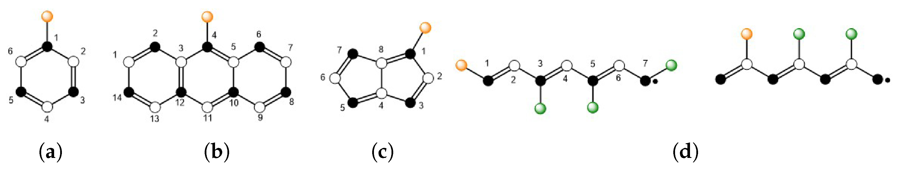
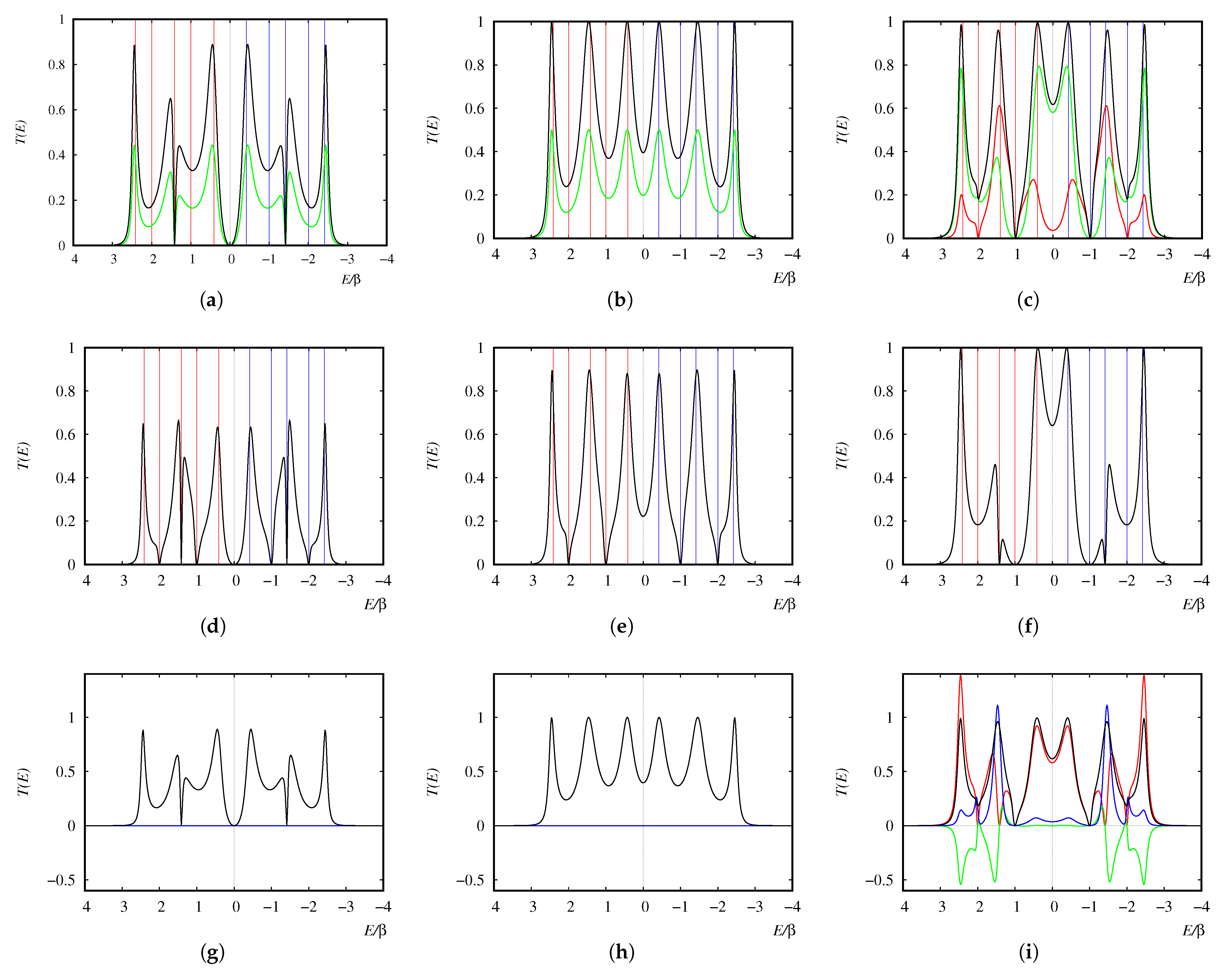
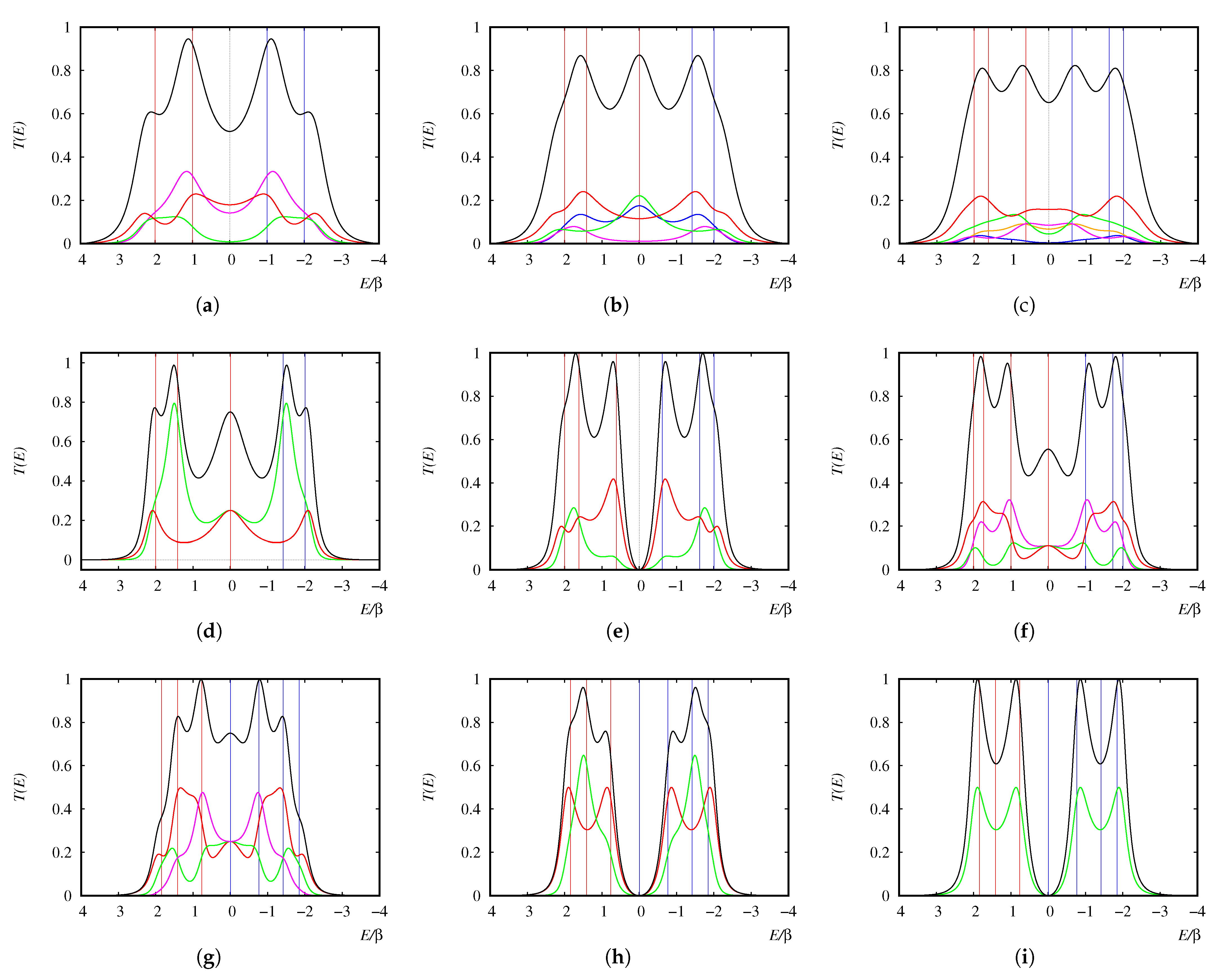
The labelling schemes for the molecules under study are shown in Figure 3. Figure 4, Figure 5, Figure 6 and Figure 7 show transmission curves plotted against electron energy. In each case, the black outer envelope is the total transmission from the source lead into the molecule, and coloured curves show (symmetry distinct) transmissions from the molecule into sink leads. A colour code is used to distinguish the leads in clockwise order from the source. The plots also indicate poles of the molecular Green’s function, using an encoding of blue for attachment and red for ionisation poles.

6.1. Devices Based on the Benzene Ring

As a first example, we take the six-membered ring of carbon atoms, which can be connected as a two-lead device in three ways (‘ortho’, ‘meta’, ‘para’) and as a three-lead device in six ways, leading to the nine transmission curves shown in Figure 4. All curves are symmetric about the Fermi energy in the Hückel model, as the six-ring is a bipartite graph. Transmission curves for the three two-lead devices are qualitatively different. The ortho and para devices have non-zero transmission at the Fermi energy, with different patterns in the wings, as predicted by the analytical expression for $T\left(E\right)$ of a cycle [55] and selection rules [61,63] for conduction at degenerate and non-degenerate eigenvalues (here, $\alpha \pm \beta$). In contrast, the meta device is insulating at the Fermi level.

Plots for the various three-lead devices show a variety of patterns, but it is striking that the overall shapes of the curves can be interpreted in terms of constituent two-lead components: to a first approximation, the curve $T\left(E\right)$ for the three-lead device with source 1, and sinks a and b has lead contributions that follow the patterns for devices $(1,a)$ and $(1,b)$ in the region of the Fermi level but are damped in the higher and lower energy wings. The implication is that the interference terms (see Equation (60)) have smooth, predictable effects on $T\left(E\right)$ for the composite device. This pattern is especially clear for the symmetric $(1,3,5)$ device (Figure 4i), where the source is in a meta relations to both sinks, and the Fermi-level transmission is zero. In fact, this device is a CBSD: interference terms between leads do not appear in the numerators of the lead currents, and the device is interference-free. In other devices such as $(1,2,3)$ and $(1,3,4)$, a vanishing Fermi-level contribution from the meta constituent device is masked by the contribution from the other constituent. The counting of ortho, meta and para constituent devices works well as a rough guide to $T\left(E\right)$, though we may expect this simplicity to be diluted in larger systems and devices with more leads.

The final row of Figure 4 shows the transmission curves calculated at the GF2 level for $(1,2)$, $(1,4)$ constituent devices, flanking the plot for the composite three-lead device $(1,2,4)$. The plots show strong resemblances to those calculated at the Hückel level, and interpretation of the lead contributions in terms of constituent devices survives intact in the correlated treatment.

6.2. Devices Based on Anthracene

This section presents results on devices based on anthracene, which, similar to benzene, has a bipartite molecular graph. The devices considered here all have three leads, with the source on atom 4 in the numbering of Figure 3. The devices for which transmission curves are shown in Figure 5a–c are (4,8,14), (4,9,13) and (4,8,11), which span the types ($•,•,•$), ($•,\circ ,\circ$), and ($•,•,\circ$), where the colours of the circles represent the partite sets (Figure 3b). All three necessarily have single-vertex deleted and triple-vertex deleted graphs that are non-Kekulean and have at least one non-Kekulean constituent two-lead device. Devices (4,8,14) and (4,9,13) are C${}_{2v}$ symmetric, and their total tramsission is simply twice the contribution of each sink lead. The second row of the Figure shows the three two-lead constituent devices (4,8), (4,9), and (4,11). In each case, there is a clear qualitative correspondence between the three-lead device and its constituent devices, i.e., (a) with (d); (b) with (e); and in the mirror-symmetric (c), the distinct lead contributions strongly resemble (f) and (d), generally as expected. Exceptions to this agreement are in the features where the transmission falls sharply to zero at eigenvalues $\pm 2$ and $\pm 1$ in the two-lead (4,8)- and (4,9) constituent devices; these are suppressed in the mirror symmetric three-wire devices as an effect of specific cancellations with the denominator.

The final row of panels Figure 5g–i refers to interference terms in lead currents in the three-lead devices. Explicit calculation of interference contributions to the numerators of the expressions for the lead currents shows that the mixed and pure interference contributions are identically zero for the mirror-symmetric devices (4,8,14) and (4,9,13) but not for the non-symmetric one (4,8,11). As shown in Figure 5i, interference terms of both mixed and pure types appear. It is risky to generalise too much from one example, but it is at least interesting to see that these terms exert little effect in the central region of the spectrum (where they are both small) but are more influential in the wings (where they are more intense and have regions of opposite sign).

6.3. A Non-Bipartite Case: Devices Based on Pentalene

Figure 6 shows a cascade of calculated curves $T\left(E\right)$ for non-bipartite (i.e., non-alternant) pentalene. We take one example of a four-lead device and compare it with all of the constituent two- and three-lead devices. The chosen four-lead case has connections at vertices 1,3,5,7 (Figure 6a), which are the four core vertices for the non-degenerate non-bonding LUMO of pentalene (i.e., they carry the non-zero charge/spin densities for this orbital).

The plots are no longer symmetric, as the spectrum of a non-bipartite graph is not paired, but there are still discernible qualitative features of the transmission curve that are associated with eigenvalues: broad or compound maxima at most eigenvalues, and a sharp spike in the transmission at the HOMO eigenvalue ($\alpha +0.47068\beta$ in Hückel theory). The plot also shows a broad dip in transmission at antibonding energies above the LUMO. The origins of the lead contributions to devices in the middle row are plausibly traced from the appropriate two-lead devices ((e) and (f) to (b); (e) and (g) to (d); (f) and (g) to (d)), and the constituent device curves for (e), (f), and (g) appear in the plot for the full device (a), with some blurring of features by interference effects. The family relationships of devices with progressively increasing numbers of leads are yet again helpful as a rough guide to the features of the transmission spectrum of a complex device.

6.4. Complete Devices of Types CSD and CBSD

Figure 7 shows calculated curves $T\left(E\right)$ for molecular devices of CSD and CBSD types based on cycles and linear polyenes. The first three panels show the transmission curves for CSD based on 6-, 8-, and 10-membered rings (Figure 7a–c). They show qualitatively similar behaviour, with broad maxima, shoulders, and minima associated with the eigenvalues of the respective graphs. The pattern of a central minimum for $(4N+2)$-rings and a central maximum for $4N$-rings persists to larger ring sizes. Traces of the constituent devices are apparent in the lead contributions, e.g., compare ortho, meta, and para benzene devices (Figure 4a–c) with the CSD in Figure 7a. As noted in Section 4.1, transmission is non-zero across the whole band window. However, the summed current can include some very low sink-lead contributions. In the case of the 10-ring, for example, the lead transmissions at the Fermi level for leads 2, 3, 4, 5, and 6 are 0.1581, 0.0445, 0.0853, 0.0042, and 0.0674, respectively.

The next three panels (Figure 7d–f) show the transmission curves for CBSD based on 8-, 10-, and 12-membered rings (Figure 7a–c). Again, a pattern of alternating behaviour at the Fermi level is apparent and is confirmed by extension of the calculations to larger rings: CBSD based on $4N$-rings show a central maximum in total transmission, consistent with superposition of sink-lead curves with central maxima, whereas $(4N+2)$-rings have an insulating minimum at the Fermi level, indicating vanishing of all lead contributions. As noted in Section 4.3, this is part of a general pattern based on the number of non-bonding orbitals (NBOs), or in other words, the nullity of the graph. In the $4N$-ring, the nullity is 2 and all centres carry non-zero density arising from any occupation of the non-bonding shell (i.e., a $4N$-ring is a core graph [82]). Cancellation of the $E^2$ factor between numerator and denominator in the expression for lead currents therefore yields conduction at the Fermi level for these rings. The $(4N+2)$-rings have no such cancellation. This convex/concave pattern for antiaromatic/aromatic rings is one example of a nullity-based selection rule for a family of devices. There will be many more to be found.

Finally, the third row (Figure 7g–i) deals with complete bipartite devices based on the heptratriene linear polyene. As shown in Figure 3, the molecular graph has two partite sets of vertices. The graph has nullity one and the unique Hückel NBO has non-zero entries only on the larger (black) partite set. This leads to a qualitative distinction between devices of CBSD type based on the two sets. For the (1,3,5,7) device, there is non-zero density in the NBO at all lead positions, and cancellation of the $E^2$ factor in the numerator leads to Fermi conduction. On the other hand, the two devices based on the smaller (white) partite set show insulation at the Fermi level, even though the underlying graph is still of course singular, as all lead positions are at nodes in the NBO.

A comparison of Figure 7h–i shows that this central feature of the transmission spectrum is independent of the choice of source lead position within the same partite set. There is, however, a significant difference between the (2,4,6)- and (4,2,6)-devices. The molecule has a mirror plane through the central vertex, so that MOs that are antisymmetric with respect to the mirror have ${\mathbf{U}}_{\mathrm{i}4}=0$. The (2,4,6)-device in panel (h) displays weak inertness for lead 2 attached to vertex 4 (in red) but not for lead 3 attached to vertex 6 (the green curve). Hence, no maximum is visible in the red curve near the second eigenvalue from the right or the second from the left. The (4,2,6)-device, in panel (i), exhibits strong inertness for these same eigenvalues because the source lead is attached to vertex 4. These observations are again indicative of the wealth of underlying selection rules.

7. Connections with the Meir–Wingreen Formula

The Meir–Wingreen (MW) formula gives an exact expression for the current through a molecular device described using a correlated molecule but with leads and lead–molecule interactions treated in the one-electron approximation. In previous work [70], we showed that the SSP method is consistent with the MW formula, in the elastic-scattering limit when the electron–phonon interactions are neglected (i.e., in the Born–Oppenheimer approximation). SSP produces identical formulae for the transmission, including the case in which the description of the central molecule includes electron correlation.

The transmission in the SMSP approach is determined by boundary conditions on a device wave function with conceptual advantages in the chemical interpretability of the internal molecular channels for conduction. These channels are determined by the attached and ionised states appearing in the Lehmann representation of the equilibrium molecular GF. The properties of these channels are defined in terms of the characteristics of the DOs associated with each of the GF poles. The sets of orbitals and poles define spectral expansions of structural polynomials used to formulate the expressions we derived in this paper. The relevant formal properties of the polynomials are retained regardless of the level of theory, from Hückel, through HF, to sophisticated GF formalisms. The molecular part of the problem may therefore be treated with empirical, semi-empirical, or ab initio methods, with or without the inclusion of correlation, thus giving a seamless single formalism to describe conduction through molecular devices.

At any of these levels of approximation, the inverse ${\left(\mathbf{P}\right)}^{-1}$ of the SSP/SMSP device matrix is the device GF (Equation (85) of [70]). The poles of this matrix are complex-valued and represent device resonances corresponding to the presence of an extra electron (or hole) in the sea of (possibly correlated) electrons. The imaginary parts of these poles are inversely related to the lifetimes of the resonances. These lifetimes represent transit times for the particles or holes crossing the device, times that are particularly short for Koopmans poles but long for shake poles. In the SMSP context, it can be seen that the poles of the device GF can be obtained by solving the equation $|{\mathrm{D}}_{\mathrm{L}}{\left(E\right)|}^2=0$. Each complex conjugate pair of poles is then associated with a Dyson orbital and (real) pole energy of the molecular GF. Hence, the SMSP model gives a direct route to calculation and interpretation of all the properties that can be accessed through GF methods.

8. Conclusions

Working equations have been derived for an extended version of the SSP model for calculation of ballistic currents flowing through molecular conductors under a potential difference. They constitute the new Source-and-Multiple-Sink Potential model. The new model describes systems with an incoming electron travelling along a single source lead that drains out through the molecule into multiple sinks. As with its SSP predecessor, SMSP lends itself to a graph-theoretical approach, which leads to a formulation that is compatible with, but not confined to the Hückel/tight-binding description of electronic structure of $\pi$ systems. SMSP therefore retains the advantages of SSP. It yields closed-form expressions for device transmission as a function of electron energy: for general lead parameters (Section 3.2); for chemically symmetric leads (Section 3.3); and for leads with coverage of all $\pi$-centres (Section 4.1), or of all starred or unstarred centres of an alternate $\pi$-system (Section 4.3).

As its SSP predecessor did, the SMSP model gives predictions for qualitative selection rules and generic patterns of conduction for families of molecular systems, such as the opposite behaviour of aromatic and anti-aromatic rings at the Fermi level (Section 6.4). In addition to a calculus for the prediction of total transmission with energy, the model allows for an analysis of molecular current at various levels of detail: by bond current, by orbital-based molecular channels, and by destination lead (Section 5). Patterns of current in multi-lead devices can be interpreted as built up from notional constituent two-lead devices, where SMSP gives a natural breakdown into direct contributions, interference terms (again governed by selection rules), and mean-field corrections (Section 3.5). The wide-band limit yields particularly simple expressions for transmission involving only the characteristic polynomials of the set of vertex-deleted graphs (Section 3.4). In the hypothetical limit of full or half coverage of a molecule by leads, the specific interference effects are predicted to vanish (Section 4.1 and Section 4.3). The symmetry of the device can also cause the vanishing of interference effects (Section 5.3) when the connection point for the sink leads are equivalent.

SMSP, similar to SSP, is a parameterised model, with two parameters ${\beta }_{\mathrm{L}}$, and ${\beta }_{\mathrm{L}\mathrm{M}}$ (defined in units of $\beta$, the resonance integral for the molecule). Adjusting the parameters affects the detailed appearance of the transmission spectrum and the relative importance of interference effects. The effective lead parameter ${\beta }_{\mathrm{L}}$ is likely to be larger in magnitude than $\beta$, even in all-carbon devices since the co-ordination number is higher with structured leads. The molecular energy levels, therefore, lie inside the band as assumed in our sample calculations. The role of ${\beta }_{\mathrm{L}\mathrm{M}}$ is to describe the perturbation of the molecule by the leads, the effect of which is to move poles of the molecular GF off the real axis, and hence, lower ${\beta }_{\mathrm{L}\mathrm{M}}$ values give sharper transmission peaks. Interference effects become more important as the ratio ${\beta }_{\mathrm{L}\mathrm{M}}^2/{\beta }_{\mathrm{L}}$ increases, as shown in (Section 3.5). Perhaps the main advantage of models such as SMSP is that many interpretative features persist when more realistic models of electronic structure are used. In particular, the analysis by molecular-orbital-based channels survives the introduction of electron–electron interaction into the theory.

Thus far, we are not aware of experimental work on molecular systems with dense attachment of leads to single molecules. Mechanically controlled break-junction (MCB) techniques [83] provide IV characteristics that give insight into averaged conduction for two-lead molecular devices rather than their detailed transmission spectra. Even so, an impressive range of data on the factors influencing molecular conductivity can be inferred from painstaking experimentation based on careful molecular design. For example, encouraging agreement with experimentally observed regiospecificity of conduction [84] can already be achieved using non-empirical and graph-theoretical SSP calculations [43,60]. The long-term aim of the present work is to carry forward this modelling of trends to multi-lead devices, in the hope that it may be of use in the design of future experiments on these intriguing systems.

References

1. Ratner, M.A. A brief history of molecular electronics. Nat. Nanotechnol. 2013, 8, 378–381. [Google Scholar] [CrossRef]
2. Cuevas, J.C.; Scheer, E. Molecular Electronics: An Introduction to Theory and Experiment; World Scientific: Singapore, 2010. [Google Scholar]
3. Datta, S. Quantum Transport: Atom to Transistor; Cambridge University Press: Cambridge, UK, 2013. [Google Scholar]
4. Stefanucci, G.; van Leeuwen, R. Nonequilibrium Many-Body Theory of Quantum Systems; Cambridge University Press: Cambridge, UK, 2013. [Google Scholar]
5. Moth-Poulsen, K. Handbook of Single-Molecule Electronics; CRC: Boca Raton, FL, USA, 2015. [Google Scholar]
6. Xanthakis, J. Electronic Conduction: Classical and Quantum Theory to Nanoelectronic Devices; CRC Press: Boca Raton, FL, USA, 2020. [Google Scholar]
7. Aviram, A.; Ratner, M.A. Molecular rectifiers. Chem. Phys. Lett. 1974, 29, 277–283. [Google Scholar] [CrossRef]
8. Caroli, C.; Combescot, R.; Noziéres, P.; Saint-James, D. Direct calculation of the tunneling current. J. Phys. C. Solid State Phys. 1971, 4, 916–929. [Google Scholar] [CrossRef]
9. Caroli, C.; Combescot, R.; Lederer, D.; Noziéres, P.; Saint-James, D. A direct calculation of the tunneling current: II. Free electron description. J. Phys. C. Solid State Phys. 1971, 4, 2598–2610. [Google Scholar] [CrossRef]
10. Caroli, C.; Combescot, R.; Noziéres, P.; Saint-James, D. A direct calculation of the tunneling current: IV. Electron-phonon effects. J. Phys. C. Solid State Phys. 1972, 5, 21–42. [Google Scholar] [CrossRef]
11. Mujica, V.; Kemp, M.; Ratner, M.A. Electron conduction in molecular wires. I. A scattering formalism. J. Chem. Phys. 1994, 101, 6849–6855. [Google Scholar] [CrossRef]
12. Mujica, V.; Kemp, M.; Ratner, M.A. Electron conduction in molecular wires. II. Application to scanning tunnelling microscopy. J. Chem. Phys. 1994, 101, 6856–6864. [Google Scholar] [CrossRef]
13. Mujica, V.; Kemp, M.; Roitberg, A.; Ratner, M. Current-voltage characteristics of molecular wires: Eigenvalue staircase, Coulomb blockade, and rectification. J. Chem. Phys. 1996, 104, 7296–7305. [Google Scholar] [CrossRef]
14. Tian, W.; Datta, S.; Hong, S.; Reifenberger, R.; Henderson, J.I.; Kubiak, C.P. Conductance spectra of molecular wires. J. Chem. Phys. 1998, 109, 2874–2882. [Google Scholar] [CrossRef]
15. Maiti, S.K. Quantum transport through polycyclic hydrocarbon molecules. Phys. Lett. A 2007, 366, 114–119. [Google Scholar] [CrossRef] [Green Version]
16. Kadanoff, L.P.; Baym, G. Quantum Statistical Mechanics; Benjamin, W.A., Ed.; CRC Press: Boca Raton, FL, USA, 1962. [Google Scholar]
17. Baym, G. Self-consistent approximations in many-body systems. Phys. Rev. 1962, 171, 1391–1401. [Google Scholar] [CrossRef]
18. Keldysh, L.V. Diagram technique for non-equilibrium processes. Zh. Eksp. Teor. Fiz. 1965, 47, 1515, translated in Sov. Phys. JETP. 1965, 20, 1018. [Google Scholar]
19. Meir, Y.; Wingreen, N.S. Landauer formula for the current through an interacting electron region. Phys. Rev. Lett. 1992, 68, 2512–2515. [Google Scholar] [CrossRef] [PubMed]
20. Heath, J.R.; Ratner, M.A. Molecular Electronics. Phys. Today 2003, 56, 43–49. [Google Scholar] [CrossRef]
21. Solomon, G.C.; Gagliardi, A.; Pecchia, A.; Frauenheim, T.; Di Carlo, A.; Reimers, J.R.; Hush, N.S. The symmetry of single-molecule conduction. J. Chem. Phys. 2006, 125, 184702. [Google Scholar] [CrossRef]
22. Paulsson, M.; Brandbyge, M. Transmission eigenchannels from nonequilibrium Green’s functions. Phys. Rev. B 2007, 76, 115117. [Google Scholar] [CrossRef] [Green Version]
23. Solomon, G.C.; Andrews, D.Q.; Hansen, T.; Goldsmith, R.H.; Wasielewski, M.R.; Van Duyne, R.P.; Ratner, M.A. Understanding quantum interference in coherent molecular conduction. J. Chem. Phys. 2008, 129, 054701. [Google Scholar] [CrossRef] [Green Version]
24. Solomon, G.C.; Andrews, D.Q.; Goldsmith, R.H.; Hansen, T.; Wasielewski, M.R.; Van Duyne, R.P.; Ratner, M.A. Quantum Interference in Acyclic Systems: Conductance of Cross-Conjugated Molecules. J. Am. Chem. Soc. 2008, 130, 17301–17308. [Google Scholar] [CrossRef]
25. Solomon, G.C.; Herrmann, C.; Hansen, T.; Mujica, V.; Ratner, M.A. Exploring local currents in molecular junctions. Nat. Chem. 2010, 2, 223–228. [Google Scholar] [CrossRef]
26. Reuter, M.G.; Solomon, G.C.; Hansen, T.; Seideman, T.; Ratner, M.A. Understanding and controlling crosstalk between parallel molecular wires. Phys. Chem. Lett. 2011, 2, 1667–1671. [Google Scholar] [CrossRef]
27. Yoshizawa, K.; Tada, T.; Staykov, A. Orbital views of the electron transport in molecular devices. J. Am. Chem. Soc. 2008, 130, 9406–9413. [Google Scholar] [CrossRef] [PubMed]
28. Tsuji, Y.; Staykov, A.; Yoshizawa, K. Molecular conductance obtained in terms of orbital densities and polarizabilities. J. Am. Chem. Soc. 2011, 133, 5955–5965. [Google Scholar] [CrossRef]
29. Tsuji, Y.; Staykov, A.; Yoshizawa, K. Orbital determining spintronic properties of a conjugated system. J. Phys. Chem. C 2012, 116, 16325–16332. [Google Scholar] [CrossRef]
30. Reuter, M.; Hansen, T.; Reuter, M.G.; Hansen, T. Communication: Finding destructive interference features in molecular transport junctions. J. Chem. Phys. 2014, 141, 181103. [Google Scholar] [CrossRef] [PubMed] [Green Version]
31. Morikawa, T.; Narita, S.; Klein, D.J. Molecular electric conductance and long-bond structure counting for conjugated-carbon nano-structures. Chem. Phys. Lett. 2005, 402, 554–558. [Google Scholar] [CrossRef]
32. Tada, T.; Yoshizawa, K. Molecular design of electron transport with orbital rule: Toward conductance-decay free molecular junctions. Phys. Chem. Chem. Phys. 2015, 17, 32099–32110. [Google Scholar] [CrossRef] [Green Version]
33. Stuyver, T.; Fias, S.; De Proft, F.; Geerlings, P. Back of the Envelope Selection Rule for Molecular Transmission: A Curly Arrow Approach. J. Phys. Chem. C 2015, 119, 26390–26400. [Google Scholar] [CrossRef]
34. Tsuji, Y.; Estrada, E.; Movassagh, R.; Hoffmann, R. Quantum Interference, Graphs, Walks, and Polynomials. Chem. Rev. 2018, 118, 4887–4911. [Google Scholar] [CrossRef] [Green Version]
35. Ernzerhof, M.; Zhuang, M. Current transport through molecular electronic devices. J. Chem. Phys. 2003, 119, 4134–4140. [Google Scholar] [CrossRef]
36. Zhuang, M.; Ernzerhof, M. Zero-voltage conductance of short gold nanowires. J. Chem. Phys. 2004, 120, 4921–4926. [Google Scholar] [CrossRef]
37. Ernzerhof, M.; Zhuang, M.; Rocheleau, P. Side-chain effects in molecular electronic devices. J. Chem. Phys. 2005, 123, 134704. [Google Scholar] [CrossRef]
38. Ernzerhof, M. Density functional theory of complex transition densities. J. Chem. Phys. 2006, 125, 124104. [Google Scholar] [CrossRef]
39. Ernzerhof, M.; Bahmann, H.; Goyer, F.; Zhuang, M.; Rochelau, P. Electron Transmission through Aromatic Molecules. J. Chem. Theory Comput. 2006, 2, 1291–1297. [Google Scholar] [CrossRef] [PubMed]
40. Goyer, F.; Ernzerhof, M.; Zhuang, M. Source and sink potentials for the description of open systems with a stationary current passing through. J. Chem. Phys. 2007, 126, 144104. [Google Scholar] [CrossRef]
41. Ernzerhof, M. A simple model of molecular electronic devices and its analytical solution. J. Chem. Phys. 2007, 127, 204709. [Google Scholar] [CrossRef]
42. Zhuang, M.; Ernzerhof, M. Reversibility and transport properties of dithienylethene photoswitches. J. Chem. Phys. 2009, 130, 114704. [Google Scholar] [CrossRef] [PubMed]
43. Rocheleau, P.; Ernzerhof, M. Molecular conductance obtained in terms of orbital densities and response functions. J. Chem. Phys. 2009, 130, 184704. [Google Scholar] [CrossRef]
44. Ernzerhof, M.; Goyer, F. Conjugated molecules described by a one-dimensional Dirac equation. J. Chem. Theory Comput. 2010, 6, 1818–1824. [Google Scholar] [CrossRef] [PubMed]
45. Zhou, Y.X.; Ernzerhof, M. Equiconducting molecular electronic devices. J. Chem. Phys. 2010, 132, 104706. [Google Scholar] [CrossRef]
46. Goyer, F.; Ernzerhof, M. Correlation effects in molecular conductors. J. Chem. Phys. 2011, 134, 174101. [Google Scholar] [CrossRef]
47. Ernzerhof, M. Simple orbital theory for the molecular electrician. J. Chem. Phys. 2011, 135, 014104. [Google Scholar] [CrossRef]
48. Rocheleau, P.; Ernzerhof, M. Extension of the source-sink potential (SSP) approach to multichannel quantum transport. J. Chem. Phys. 2012, 137, 174112. [Google Scholar] [CrossRef]
49. Zhou, Y.; Ernzerhof, M. Open-system Kohn-Sham density functional theory. J. Chem. Phys. 2012, 136, 094105. [Google Scholar] [CrossRef]
50. Mayou, D.; Zhou, Y.; Ernzerhof, M. The zero-voltage conductance of Nanographenes: Simple rules and quantitative estimates. J. Phys. Chem. C 2013, 117, 7870–7884. [Google Scholar] [CrossRef]
51. Ernzerhof, M. Coherent molecular transistor: Control through variation of the gate wave function. J. Chem. Phys. 2014, 140, 114708. [Google Scholar] [CrossRef] [PubMed]
52. Ernzerhof, M.; Bélanger, M.A.; Mayou, D.; Aram, T.N. Simple model of a coherent molecular photocell. J. Chem. Phys. 2016, 144, 134102. [Google Scholar] [CrossRef] [Green Version]
53. Aram, T.; Asgari, A.; Mayou, D.; Aram, T.N.; Asgari, A.; Ernzerhof, M.; Quémerais, P.; Mayou, D.; Guillemoles, J.F. Quantum modeling of two-level photovoltaic systems. EPJ Photovoltaics 2017, 8, 85503. [Google Scholar] [CrossRef]
54. Giguére, A.; Ernzerhof, M. Extending the source—Sink potential method to include electron—Nucleus coupling. J. Chem. Phys. 2021, 155, 014110. [Google Scholar] [CrossRef]
55. Pickup, B.T.; Fowler, P.W. An analytic model for steady-state currents in conjugated systems. Chem. Phys. Lett. 2008, 459, 198–202. [Google Scholar] [CrossRef]
56. Ando, T. Quantum point contacts in magnetic fields. Phys. Rev. B Condens. Matter 1991, 44, 8017–8027. [Google Scholar] [CrossRef]
57. Khomyakov, P.; Brocks, G.; Karpan, V.; Zwierzycki, M.; Kelly, P.J. Conductance calculations for quantum wires and interfaces: Mode matching and Green’s functions. Phys. Rev. B Condens. Matter Mater. Phys. 2005, 72, 035450. [Google Scholar] [CrossRef] [Green Version]
58. Varga, K.; Pantelides, S. Quantum transport in molecules and nanotube devices. Phys. Rev. Lett. 2007, 98, 076804. [Google Scholar] [CrossRef] [PubMed]
59. Cook, B.G.; Dignard, P.; Varga, K. Calculation of electron transport in multiterminal systems using complex absorbing potentials. Phys. Rev. B Condens. Matter Mater. Phys. 2011, 83, 205105. [Google Scholar] [CrossRef] [Green Version]
60. Fowler, P.W.; Pickup, B.T.; Todorova, T.Z.; Myrvold, W. A selection rule for molecular conduction. J. Chem. Phys. 2009, 131, 044104. [Google Scholar] [CrossRef]
61. Fowler, P.W.; Pickup, B.T.; Todorova, T.Z.; Myrvold, W. Conduction in graphenes. J. Chem. Phys. 2009, 131, 244110. [Google Scholar] [CrossRef]
62. Fowler, P.W.; Pickup, B.T.; Todorova, T.Z.; Pisanski, T. Fragment analysis of single-molecule conduction. J. Chem. Phys. 2009, 130, 174708. [Google Scholar] [CrossRef]
63. Pickup, B.T.; Fowler, P.W.; Borg, M.; Sciriha, I. A new approach to the method of source-sink potentials for molecular conduction. J. Chem. Phys. 2015, 143, 194105. [Google Scholar] [CrossRef] [Green Version]
64. Pickup, B.T.; Fowler, P.W.; Sciriha, I. The Hückel SSP theory of the Pauli Spin Blockade of molecular electronic devices. J. Chem. Phys. 2016, 145, 204113. [Google Scholar] [CrossRef] [PubMed] [Green Version]
65. Fowler, P.W.; Pickup, B.T.; Todorova, T.Z. Equiconducting molecular conductors. Chem. Phys. Lett. 2008, 465, 142–146. [Google Scholar] [CrossRef]
66. Fowler, P.W.; Pickup, B.T.; Todorova, T.Z.; De Los Reyes, R.; Sciriha, I. Omni-conducting fullerenes. Chem. Phys. Lett. 2013, 568–569, 33–35. [Google Scholar] [CrossRef]
67. Fowler, P.W.; Pickup, B.T.; Todorova, T.Z.; Borg, M.; Sciriha, I. Omni-conducting and omni-insulating molecules. J. Chem. Phys. 2014, 140, 054115. [Google Scholar] [CrossRef] [PubMed] [Green Version]
68. Fowler, P.W.; Sciriha, I.; Borg, M.; Seville, V.E.; Pickup, B.T. Near omni-conductors and insulators: Alternant hydrocarbons in the SSP model of ballistic conduction. J. Chem. Phys. 2017, 147, 164115. [Google Scholar] [CrossRef] [PubMed] [Green Version]
69. Fowler, P.W.; Borg, M.; Pickup, B.T.; Sciriha, I. Molecular graphs and molecular conduction: The d-omni-conductors. Phys. Chem. Chem. Phys. 2020, 22, 1349–1358. [Google Scholar] [CrossRef] [PubMed]
70. Pickup, B.T.; Fowler, P.W. A Correlated Source-Sink-Potential Model Consistent with the Meir-Wingreen Formula. J. Phys. Chem. A 2020, 124, 6928–6944. [Google Scholar] [CrossRef]
71. Landauer, R. Spatial variation of currents and fields due to localized scatterers in metallic conduction. IBM J. Res. Dev. 1957, 1, 223–231. [Google Scholar] [CrossRef]
72. Büttiker, M. Four-terminal phase-coherent conductance. Phys. Rev. Lett. 1986, 57, 1761–1764. [Google Scholar] [CrossRef] [PubMed]
73. Papior, N.; Lorente, N.A.; Frederiksen, T.; García, A.; Brandbyge, M. Improvements on non-equilibrium and transport Green function techniques: The next-generation transiesta. Comput. Phys. Commun. 2017, 212, 8–24. [Google Scholar] [CrossRef] [Green Version]
74. Sylvester, J.J. On the relation between the minor determinants of linearly equivalent quadratic functions. Philos. Mag. 1851, 1, 295. [Google Scholar] [CrossRef]
75. Brualdi, R.; Schneider, H. Determinantal Identities: Gauss, Schur, Cauchy, Sylvester, Kronecker, Jacobi, Binet, Laplace, Muir and Cayley. Linear Algebra Its Appl. 1983, 52–53, 769–791. [Google Scholar] [CrossRef]
76. Binet, J. Mémoire sur un système du formules analytiques, et leur application à des considérations géométriques. J. l’École Polytech. 1813, 9, 280–354. [Google Scholar]
77. Cauchy, A.L. Mémoire sur les fonctions qui ne peuvent obtenir que deux valeurs égales et de signes contraires par suite des transpositions operées entre les variables qu’elles renferment. J. L’École Polytech. 1815, 10, 29–112. [Google Scholar]
78. Holtz, O.; Sturmfels, B. Hyperdeterminantal relations among symmetric principal minors. J. Algebra 2007, 316, 634–648. [Google Scholar] [CrossRef] [Green Version]
79. Coulson, C.A.; Rushbrooke, G.S. Note on the method of molecular orbitals. Proc. Camb. Phil. Soc. 1940, 36, 193–200. [Google Scholar] [CrossRef]
80. Mallion, R.; Rouvray, D.H. The golden jubilee of the Coulson-Rushbrooke pairing theorem. J. Math. Chem. 1990, 5, 1–21. [Google Scholar] [CrossRef]
81. Maplesoft, Waterloo Maple Inc. Maple; Maplesoft, Waterloo Maple Inc.: Waterloo, ON, Canada, 2019. [Google Scholar]
82. Sciriha, I.; Gutman, I. Nut Graphs: Maximally Extending Cores. Util. Math. 1998, 54, 257–272. [Google Scholar]
83. Li, Z.; Smeu, M.; Park, T.H.; Rawson, J.; Xing, Y.; Therien, M.J.; Ratner, M.A.; Borguet, E. Hapticity-Dependent Charge Transport through Carbodithioate-Terminated [5,15-Bis(phenylethynyl)porphinato]zinc(II) Complexes in Metal–Molecule–Metal Junctions. Nano Lett. 2014, 14, 5493–5499. [Google Scholar] [CrossRef]
84. Web, H.; Reichert, J.; Elbing, M.; von Hanisch, C.; Beckmann, D.; Mayor, M. Electric Current through a Molecular Rod—Relevance of the Position of the Anchor Groups. Angew. Chem. Int. Ed. Engl. 2003, 42, 5834–5838. [Google Scholar]
Figure 1. The SSP model of a molecular device. (a) The full system: a molecule attached to two semi-infinite leads via single-atom connections. Black and grey vertices are conjugated π centres within the molecular region; gold vertices are on the leads. (b) The SSP graph: Left (source) and right (sink) leads are replaced by pseudo-atoms L and R linked, respectively, to atoms L ¯ and R ¯ within the molecule. Black vertices are molecular centres directly attached to leads. Grey vertices are molecular vertices that are not directly linked to a lead. Resonance integrals are β L , β R for lead-molecule contacts, β M for internal edges of the molecular graph, and β L , β R within the leads themselves. Incoming and transmitted electron waves have wavevectors q L and q R .
Applsci 11 11696 g001
Figure 2. The SMSP model of a molecular device. (a) The full system: a molecule attached to l semi-infinite leads via single-atom connections. Black and grey vertices are conjugated π centres within the molecular region; gold vertices are centres on the leads. (b) The SMSP graph: Each lead is replaced by a pseudo-atom with the index p = 1 , , l , where lead 1 is the source and all others are sinks. Black vertices are molecular centres directly attached to leads and indexed correspondingly. Grey vertices are molecular vertices that are not directly linked to a lead and are indexed l + 1 , , n .
Applsci 11 11696 g002
Figure 3. Numbering schemes for the molecules used here in examples of multi-lead devices. They are (a) benzene, (b) anthracene, (c) pentalene, and(d) heptatriene. The gold pseudo-atom symbol shows the position of the source lead; the positions of sink leads are given by the device specifications in the text. Green pseudo-atoms in (d) show the sink leads for two possible CBSD.
Applsci 11 11696 g003
Figure 4. Transmission curves for multi-lead devices based on benzene: Hückel theory results for (a) 1,2-; (b) 1,3-; (c) 1,4-; (d) 1,2,3-; (e) 1,2,4-; (f) 1,2,5-; (g) 1,2,6-; (h) 1,3,4-; and (i) 1,3,5-attachments of leads; GF2 results for (j) 1,2,-; (k) 1,2,4-; and (l) 1,4-devices. Lead 1 is the source, with transmission equal to the total envelope, shown in black. Transmissions for the second and third leads (counting clockwise in the numbering scheme of Figure 3) are shown in red and green, respectively. In the case of repetition of identical curves, later colours overwrite earlier ones. Red vertical lines show positions of ionisation poles, whilst blue lines mark attachment pole positions (in either Hückel or second-order correlated GF calculations). Dotted vertical lines mark shake poles for the correlated calculations. Lead and connection parameters are β L = 2.0 and β L M = 1 .
Applsci 11 11696 g004
Figure 5. Transmission curves for devices based on anthracene: Hückel theory results for (a) 4,8,14-; (b) 4,9,13-; (c) 4,8,11-; (d) 4,8-; (e) 4,9-; and (f) 4,11-devices. Lead 1 is the source, with transmission equal to the total envelope, shown in black. Transmissions for the second and third leads (counting clockwise in the numbering scheme of Figure 3) are shown in red and green, respectively. In the case of repetition of identical curves, later colours overwrite earlier ones. Red vertical lines show positions of ionisation poles, whilst blue lines mark attachment pole positions. Analysis of interference terms is shown for the source lead in (g) 4,8,14-; (h) 4,9,13-; and (i) 4,8,11-devices. Total transmission is shown in black, the direct term is shown in red, and mixed and pure interference terms are shown in green and blue, respectively. The lead and connection parameters are β L = 2.0 and β L M = 1.0 .
Applsci 11 11696 g005
Figure 6. Transmission curves for devices based on pentalene: Hückel theory results for (a) 1,3,5,7,-; (b) 1,3,5-; (c) 1,3,5-; (d) 1,3,7-; (e) 1,3-; (f) 1,5-; and (g) 1,7-devices. Lead 1, at vertex 3 in all cases, is the source with transmission equal to the total envelope, shown in black. Transmissions for the second, third, and fourth leads (in the numbering scheme of Figure 3) are shown in red, green, and magenta, respectively. In the case of repetition of identical curves, later colours overwrite earlier ones. Red vertical lines show positions of ionisation poles, whilst blue lines mark attachment pole positions. The lead and connection parameters are β L = 2.0 and β L M = 1.0 .
Applsci 11 11696 g006
Figure 7. Complete symmetric and complete bipartite symmetric devices. Complete symmetric devices based on (a) the C 6 ring, (b) the C 8 ring, and (c) the C 10 ring. Complete bipartite symmetric devices based on (d) the C 8 ring, (e) the C 10 ring, and (f) the C 12 ring. Complete bipartite symmetric devices based on heptatriene: (g) the (1,3,5,7)-device, (h) the (2,4,6)-device, and (i) the (4,2,6)-device. (In each case, Lead 1 is the source, with transmission shown in black. The full palette of colours is red, green, magenta, blue, and orange for sink leads, working clockwise from the source. In the case of repetition of identical curves, later colours overwrite earlier ones. For all plots, β L = 2.0 and β L M = 1 .
Applsci 11 11696 g007
Publisher’s Note: MDPI stays neutral with regard to jurisdictional claims in published maps and institutional affiliations.