
A Mathematical Model of the Production Inventory Problem for Mixing Liquid Considering Preservation Facility

 , , ,
, , ,  ,
,
Abstract
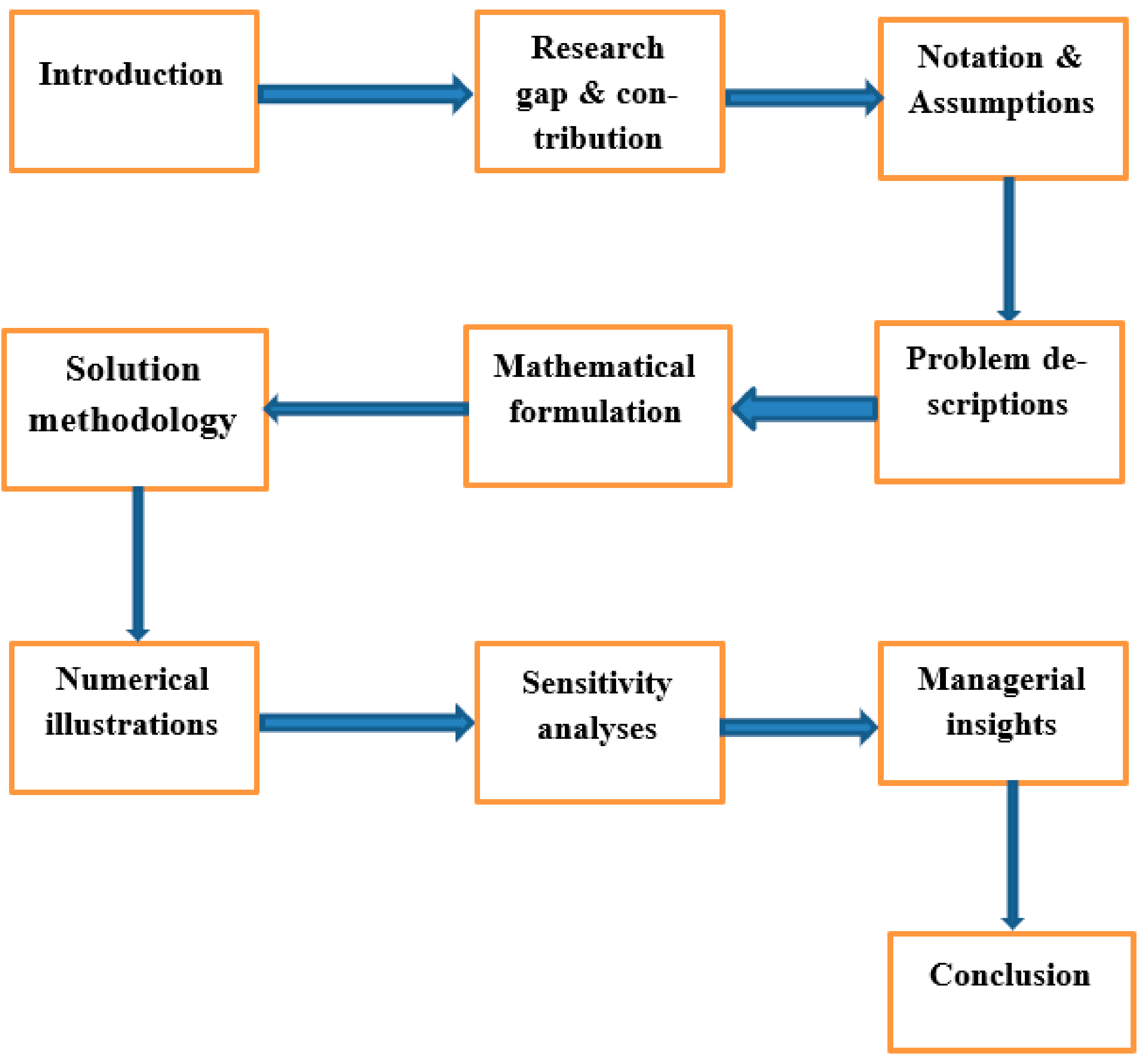
:1. Introduction
2. Research Gap and Contributions
- (i).
- Application of simultaneous linear differential equations (to the present mixing process) in the production inventory system.
- (ii).
- Linkage between the mixing process and manufacturing process.
- (iii).
- Consideration of the variable production rate in the manufacturing process dependent upon the stock level of mixed liquid.
3. Notation and Assumptions
3.1. Notation
| Concentration of liquid at time t in container-I (%) | |
| Concentration of liquid at time t in container-II (%) | |
| Stock level of mixed liquid (L) | |
| Capacity of container-I (L) | |
| Capacity of container-II (L) | |
| Incoming rate of liquid with concentration k in container-I (L/unit time) | |
| Outgoing rate of liquid from container-I to container-II (L/unit time) | |
| Incoming rate of liquid from container-II to container-I (L/unit time) | |
| Outgoing rate of liquid 2 from container-II (L/unit time) | |
| Initial concentration of liquid in container-II (%) | |
| Concentration of liquid supplied from outside (%) | |
| Demand parameters | |
| Demand of the customers | |
| Production rate (L/time unit) | |
| Wastage rate during production without preservation | |
| m | Preservation controlling parameter |
| Preservation investment ($) | |
| Processing cost ($/L) | |
| Selling price per unit ($/L) | |
| Set up cost ($/order) | |
| Carrying cost per unit per unit time ($/L/time unit) | |
| Duration of production (time unit) | |
| Cycle length (time unit) | |
| Average profit ($/time unit) |
3.2. Assumptions
- (i).
- This work deals with a mixture of three different concentrations of a liquid.
- (ii).
- The capacity of container-I filled with liquid with an initial concentration of zero (container) is less than the capacity of container-II filled with liquid with an initial concentration of k.
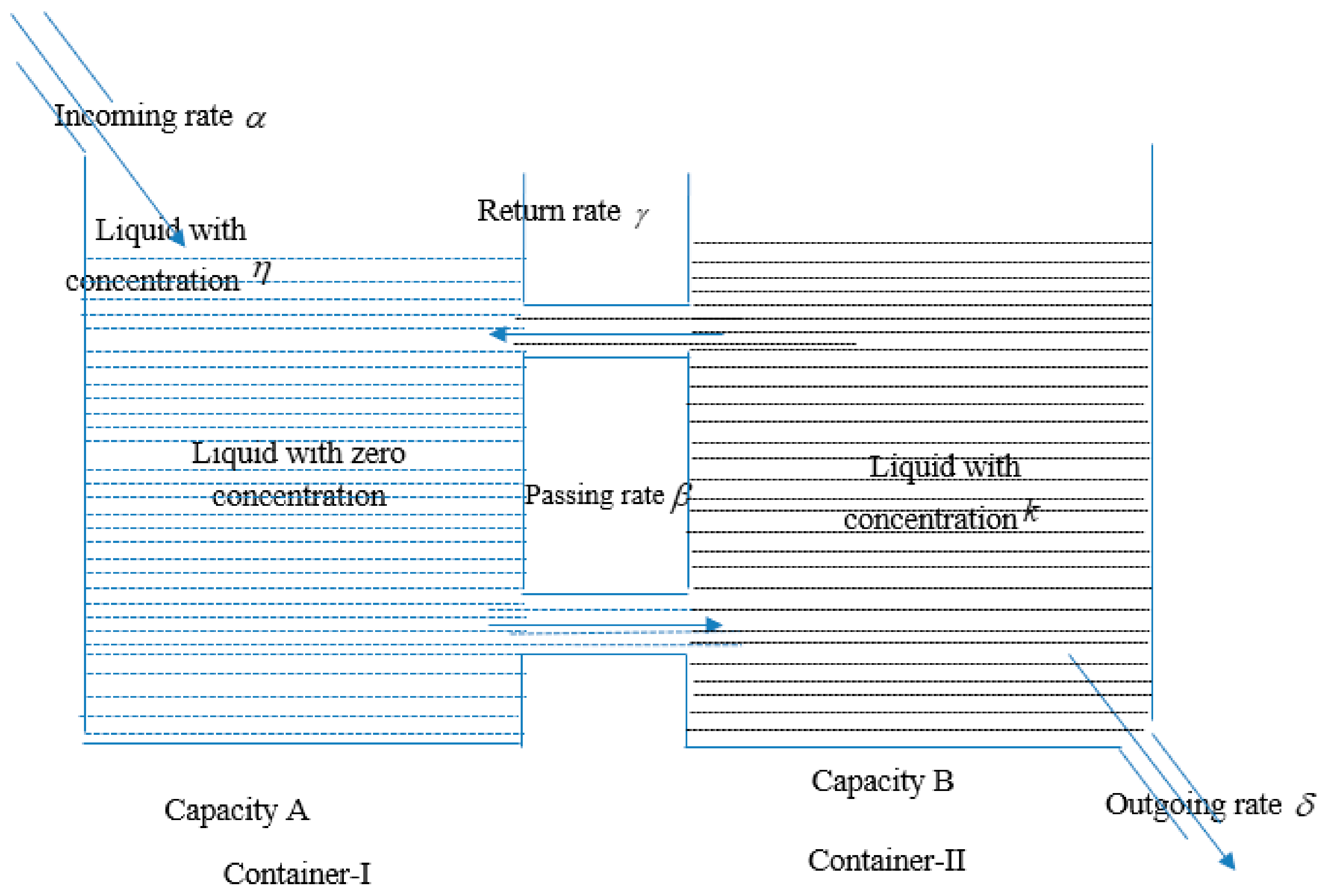
- (iii).
- At first, the liquid with concentration is sent to container-I at the rate . Then, the mixture of liquid is sent to container-II at the rate , and the liquid is sent back to container-I from container-II at the rate ; this process continues to obtain the best desirable mixture. After reaching the desired mixture, the mixed liquid from container-II at the rate is used in the production process.
- (iv).
- The production rate of the mixed product is proportional to the level of mixed liquids (y(t)). The mathematical form of is .
- (v).
- The wastage/deterioration rate during production is dependent on preservation technology. The mathematical form of the deterioration rate is , where is the preservation investment, m is the preservation controlling parameter, and is the original deterioration rate.
- (vi).
- The demand of an item is dependent on selling price and its mathematical form is , such that .
- (vii).
- Shortages are not allowed.
- (viii).
- Time horizon is infinite and lead time is constant.
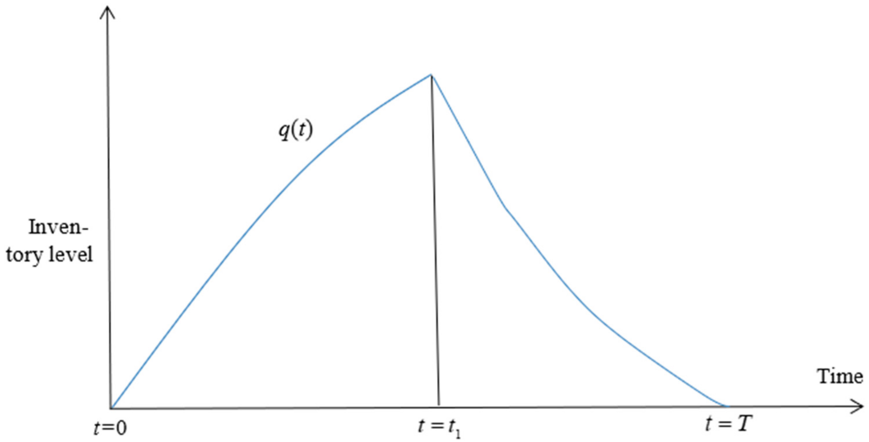
4. Problem Description
5. Mathematical Formulation
5.1. Mathematical Formulation of Mixing Problem
5.2. Mathematical Formulation of the Production Problem
5.3. Various Components of the System
- (i).
- Sales revenue (SR):
- (ii).
- Ordering cost ():
- (iii).
- Holding cost (HC):
- (iv).
- Production cost (PC):
- (v).
- Preservation cost: .
6. Solution Methodology
- (i)
- Differential evolution (Price, 1996);
- (ii)
- Simulated annealing (Marchesi, 1988).
- The initial positions of the population of size m are
- In the evaluation process for each iteration, the algorithm generates a new population with m points. Using the three points , the algorithm generated the new point randomly from the previous population.
- The mathematical form is where s is a scaling parameter.
- The new point is created from with the help of the coordinate from along with probability , otherwise it will take the coordinate from .
- If then replaces in the new population.
- The probability is controlled by the “cross probability” option.
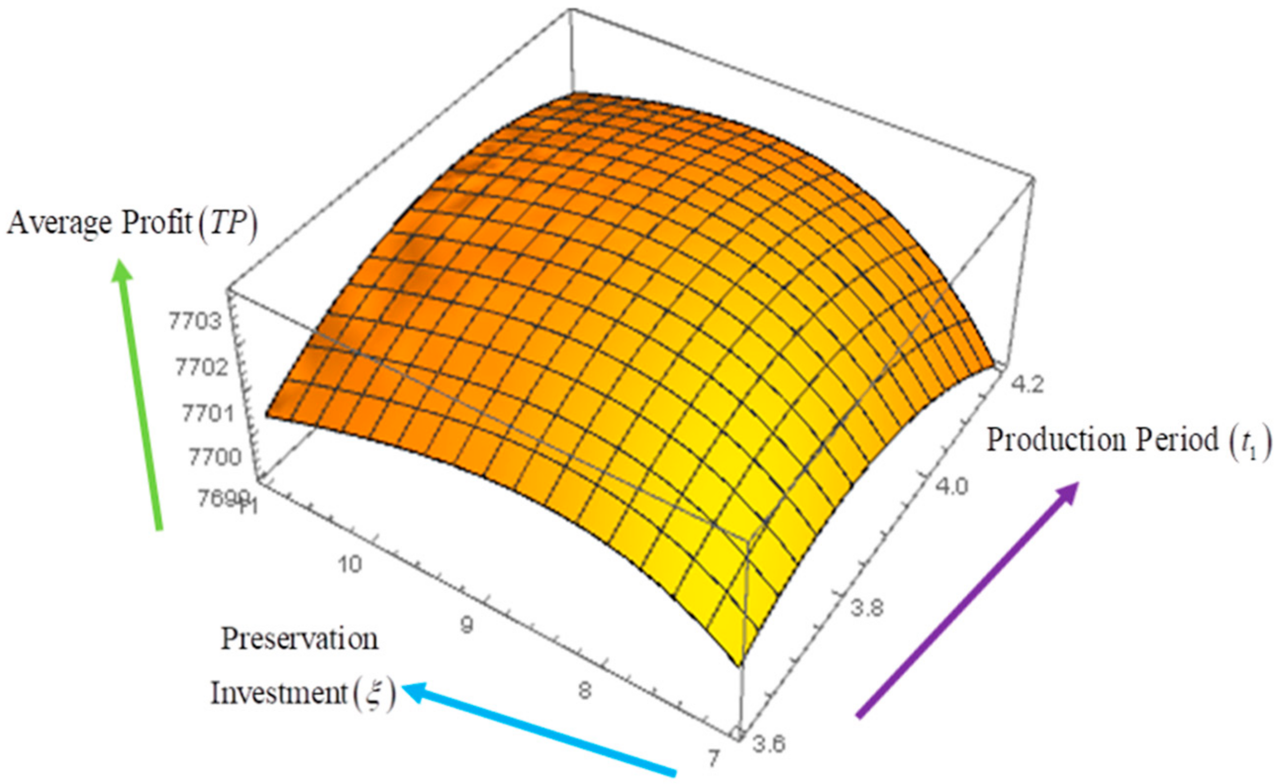
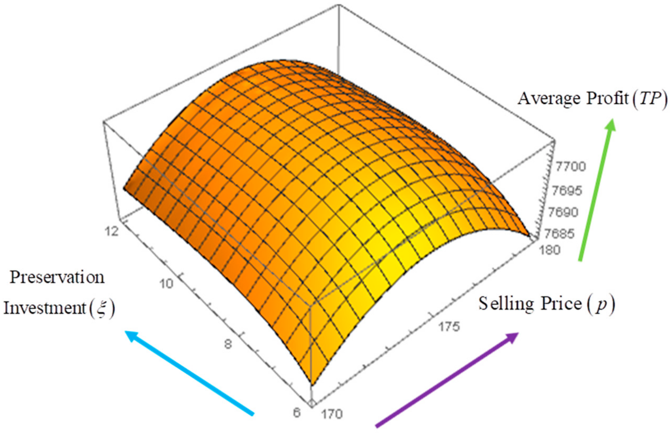
7. Numerical Illustrations
Discussion
- (i)
- The average profit of Example 2 (model with preservation technology) is higher than that of the Example 1 (model without preservation technology). From this finding, it may be concluded that the model with preservation technology is more economical than the model without preservation technology.
- (ii)
- The best-found results of both Examples 1 and 2 obtained by DE and SA are same up to a certain degree of accuracy. Thus, from here, it can also be concluded that both of the algorithms are equally efficient to solve the corresponding optimization problem of the proposed model.
- (iii)
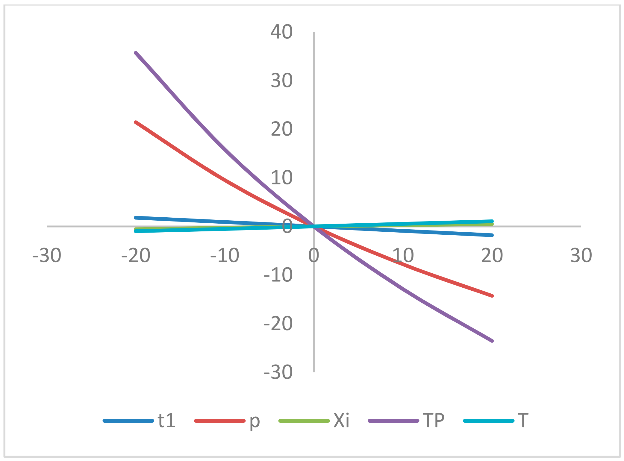
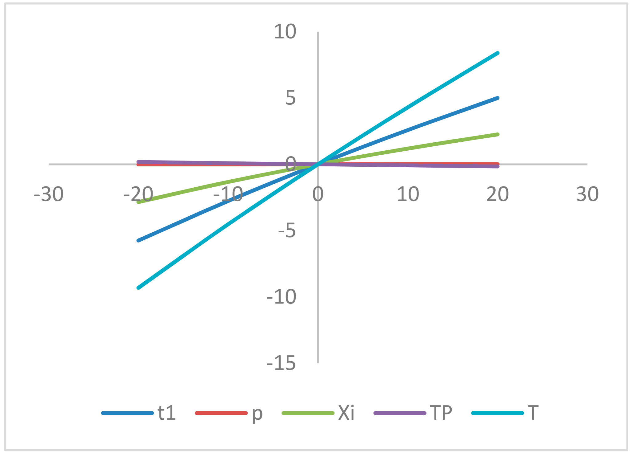
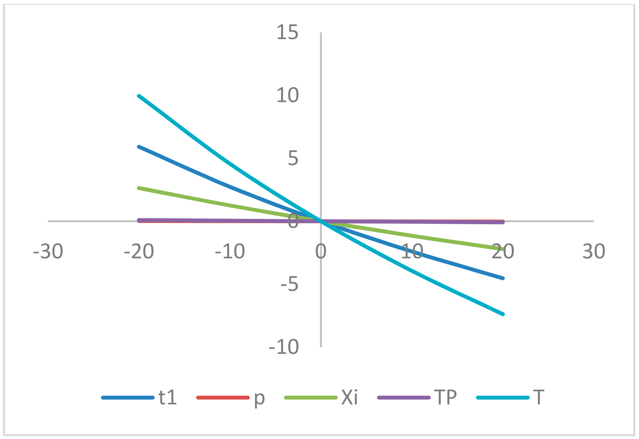
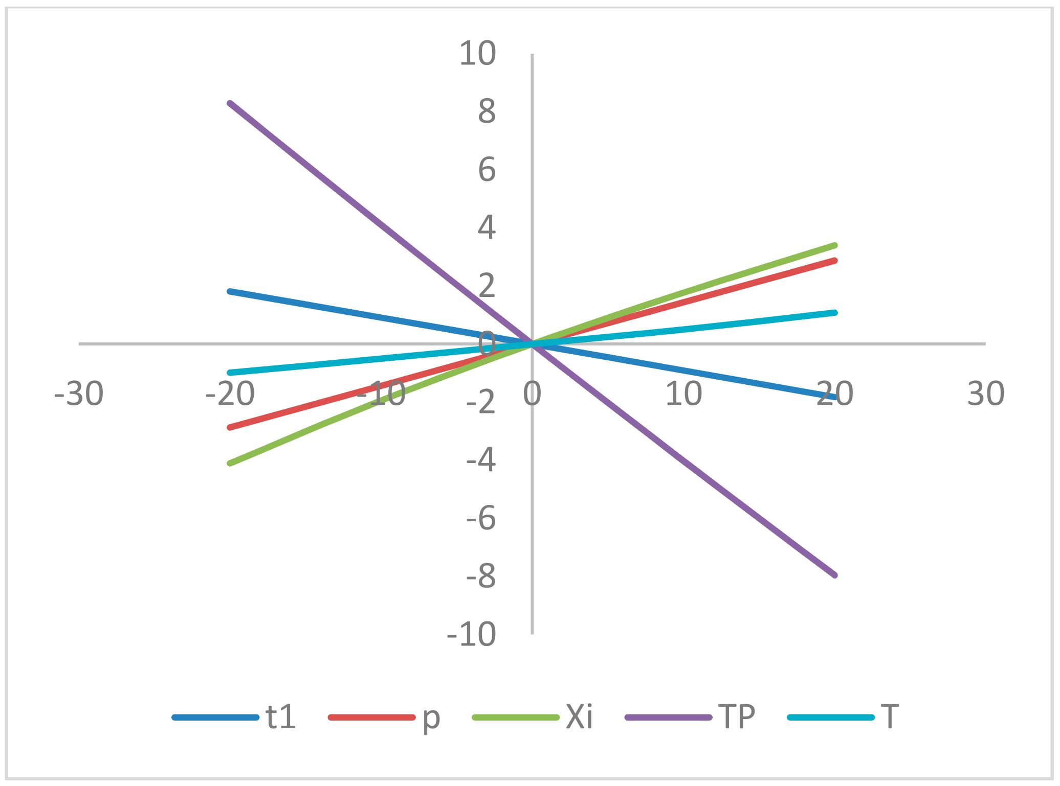
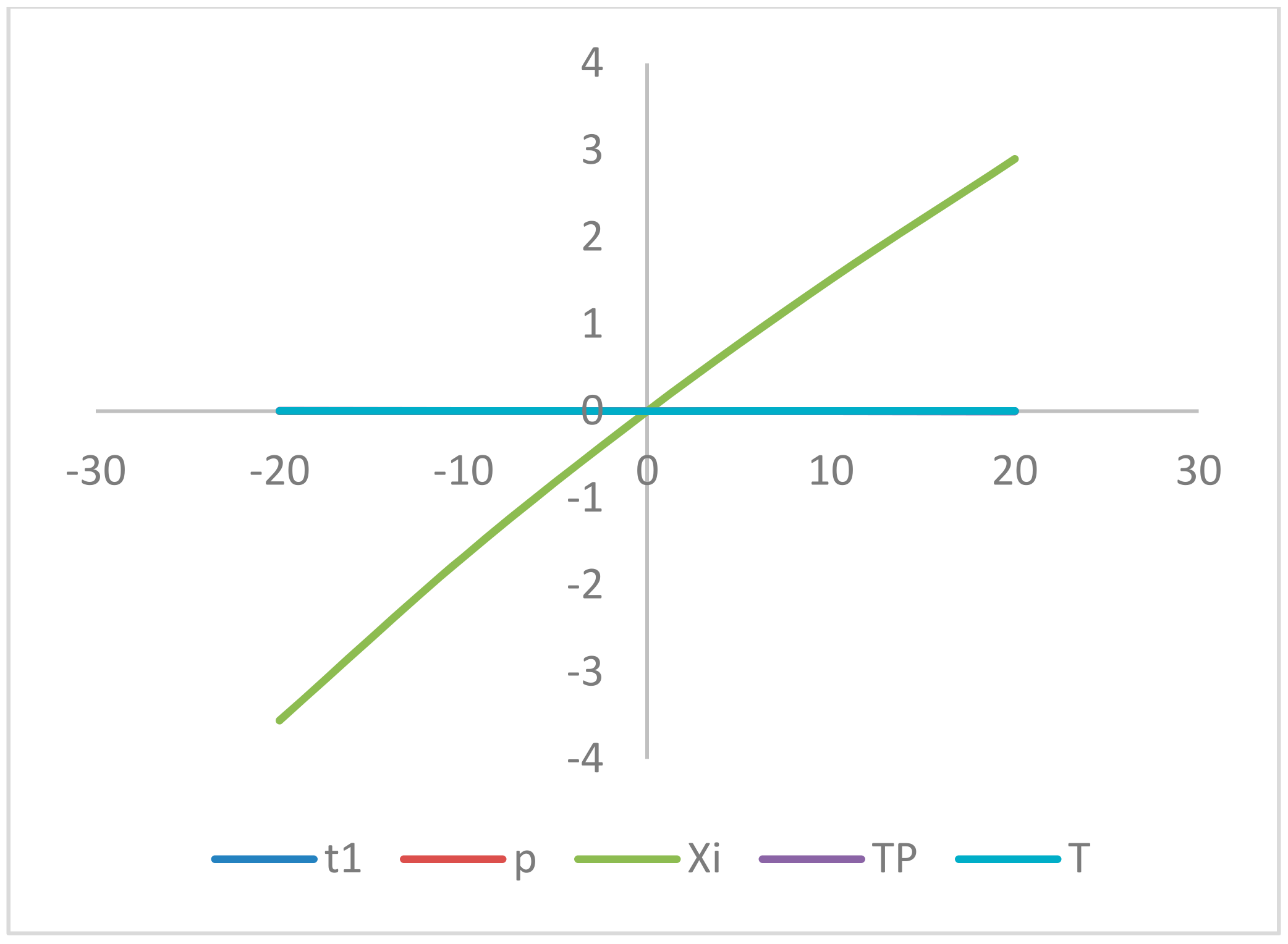
8. Sensitivity Analyses
- The profit per unit (TP) is moderately sensitive with a reverse effect with respect to , whereas it is insensitive with the change of , and highly sensitive with a reverse effect with respect to .
- The production time (t1) is less sensitive directly with respect to , and slightly sensitive with a reverse effect with respect to . On the other hand, it is insensitive with the changes in .
- The selling price (p) is slightly sensitive with respect to whereas it is insensitive with the changes in , and fairly sensitive with a reverse effect with respect to .
- The preservation investment () is slighter sensitive with respect to , whereas it is insensitive with the changes in , and highly sensitive with a reverse effect with respect to .
- The cycle length (T) is slightly sensitive with respect to , and moderately sensitive with a reverse effect with respect to h. On the other hand, it is insensitive with the changes in and fairly sensitive with respect to .
9. Managerial Implications
- (i).
- As the model with preservation technology is more economical than the model without preservation technology, it will be a good choice for the manager to consider the preservation facility during the manufacturing process of perishable products.
- (ii).
- On the other hand, the manager should be careful about the preservation controlling factor , which has a high reverse effect on the preservation investment, the ignorance of which may be the cause of higher compensation on preservation technology.
- (iii).
- The average profit is highly sensitive with respect to the demand controlling parameter and inventory cost components in the reverse sense, thus a manager/model analyst should take more care about these parameters when making the optimal decision.
10. Conclusions
Author Contributions
Funding
Institutional Review Board Statement
Informed Consent Statement
Data Availability Statement
Conflicts of Interest
References
- Gautam, C.S.; Utreja, A.; Singal, G.L. Spurious and counterfeit drugs: A growing industry in the developing world. Postgrad. Med. J. 2009, 85, 251–256. [Google Scholar] [CrossRef] [PubMed]
- Essi, D.F. Mixing Dinner and Drugs—Is It Ethically Contraindicated? AMA J. Ethics 2015, 17, 787–795. [Google Scholar] [PubMed] [Green Version]
- Ploypetchara, N.; Suppakul, P.; Atong, D.; Pechyen, C. Blend of polypropylene/poly (lactic acid) for medical packaging application: Physicochemical, thermal, mechanical, and barrier properties. Energy Procedia 2014, 56, 201–210. [Google Scholar] [CrossRef] [Green Version]
- Bernardo, F.P.; Saraiva, P.M. Integrated process and product design optimization: A cosmetic emulsion application. In Computer Aided Chemical Engineering; Elsevier: Amsterdam, The Netherlands, 2005; Volume 20, pp. 1507–1512. [Google Scholar]
- Kim, K.-M.; Oh, H.M.; Lee, J.H. Controlling the emulsion stability of cosmetics through shear mixing process. Korea-Aust. Rheol. J. 2020, 32, 243–249. [Google Scholar] [CrossRef]
- Zhang, X.; Zhou, T.; Ng, K.M. Optimization-based cosmetic formulation: Integration of mechanistic model, surrogate model, and heuristics. AIChE J. 2021, 67, 17064. [Google Scholar] [CrossRef]
- Funt, J.M. Mixing of Rubber. 2009. Available online: https://ccsuniversity.ac.in/ccsu/syllabus_camp/379syl.pdf (accessed on 13 August 2021).
- Wu, J.; Graham, L.; Nguyen, B. Mixing intensification for the mineral industry. Can. J. Chem. Eng. 2010, 88, 447–454. [Google Scholar] [CrossRef]
- Jasikova, D.; Kotek, M.; Kysela, B.; Sulc, R.; Kopecky, V. Compiled visualization with IPI method for analysing of liquid liquid mixing process. In Proceedings of the EPJ Web of Conferences, Mikulov, Czech Republic, 21–24 November 2018; Volume 180, p. 02039. [Google Scholar]
- Nienow, A.W.; Edwards, M.F.; Harnby, N. Mixing in the Process Industries. 1997. Available online: https://books.google.com.hk/books?hl=zh-CN&lr=&id=LxdFnHQcXhgC&oi=fnd&pg=PP1&dq=10.%09Nienow,+A.W.%3B+Edwards,+M.F.%3B+Harnby,+N.+Mixing+in+the+process+industries.+In+Butterworth-Heinemann%3B+1997.&ots=IbEy8GkBXx&sig=FqlgYuB327J9lHv5lBqZSs9ERy4&redir_esc=y&hl=zh-CN&sourceid=cndr#v=onepage&q=10.%09Nienow%2C%20A.W.%3B%20Edwards%2C%20M.F.%3B%20Harnby%2C%20N.%20Mixing%20in%20the%20process%20industries.%20In%20Butterworth-Heinemann%3B%201997.&f=false (accessed on 13 August 2021).
- Cheng, D.; Feng, X.; Cheng, J.; Yang, C. Numerical simulation of macro-mixing in liquid–liquid stirred tanks. Chem. Eng. Sci. 2013, 101, 272–282. [Google Scholar] [CrossRef]
- Fitschen, J.; Hofmann, S.; Wutz, J.; Kameke, A.; Hoffmann, M.; Wucherpfennig, T.; Schlüter, M. Novel evaluation method to determine the local mixing time distribution in stirred tank reactors. Chem. Eng. Sci. X 2021, 10, 100098. [Google Scholar] [CrossRef]
- De Kok, A.G. Approximations for operating characteristics in a production-inventory model with variable production rate. Eur. J. Oper. Res. 1987, 29, 286–297. [Google Scholar] [CrossRef]
- Su, C.T.; Lin, C.W. A production inventory model for variable demand and production. Yugosl. J. Oper. Res. 1999, 9, 197–206. [Google Scholar]
- Su, C.T.; Lin, C.W. A production inventory model which considers the dependence of production rate on demand and inventory level. Prod. Plan. Control 2001, 12, 69–75. [Google Scholar] [CrossRef]
- Giri, B.C.; Yun, W.; Dohi, T. Optimal design of unreliable production–inventory systems with variable production rate. Eur. J. Oper. Res. 2005, 162, 372–386. [Google Scholar] [CrossRef]
- Roy, A.; Maity, K.; Kar, S.; Maiti, M. A production–inventory model with remanufacturing for defective and usable items in fuzzy-environment. Comput. Ind. Eng. 2009, 56, 87–96. [Google Scholar] [CrossRef]
- Sana, S.S. A production-inventory model of imperfect quality products in a three-layer supply chain. Decis. Support Syst. 2011, 50, 539–547. [Google Scholar] [CrossRef]
- Sharmila, D.; Uthayakumar, R. An inventory model with three rates of production rate under stock and time dependent demand for time varying deterioration rate with shortages. Int. J. Adv. Eng. Manag. Sci. 2016, 9, 2. [Google Scholar]
- Patra, K.; Maity, R. A Single Item Inventory Model with Variable Production Rate and Defective Items. Int. J. Appl. Comput. Math. 2017, 3, 19–29. [Google Scholar] [CrossRef]
- Dey, O. A fuzzy random integrated inventory model with imperfect production under optimal vendor investment. Oper. Res. 2019, 19, 101–115. [Google Scholar] [CrossRef]
- Mishra, U.; Wu, J.-Z.; Sarkar, B. A sustainable production-inventory model for a controllable carbon emissions rate under shortages. J. Clean. Prod. 2020, 256, 120268. [Google Scholar] [CrossRef]
- Lu, C.-J.; Yang, C.-T.; Yen, H.-F. Stackelberg game approach for sustainable production-inventory model with collaborative investment in technology for reducing carbon emissions. J. Clean. Prod. 2020, 270, 121963. [Google Scholar] [CrossRef]
- Öztürk, H. Optimal production run time for an imperfect production inventory system with rework, random breakdowns and inspection costs. Oper. Res. 2021, 21, 167–204. [Google Scholar] [CrossRef]
- Khara, B.; Mondal, S.K.; Dey, J.K. An imperfect production inventory model with advance payment and credit period in a two-echelon supply chain management. RAIRO-Oper. Res. 2021, 55, 189–211. [Google Scholar] [CrossRef]
- Malik, A.I.; Sarkar, B. Disruption management in a constrained multi-product imperfect production system. J. Manuf. Syst. 2020, 56, 227–240. [Google Scholar] [CrossRef] [PubMed]
- Lin, H.J. An economic production quantity model with backlogging and imperfect rework process for uncertain demand. Int. J. Prod. Res. 2021, 59, 467–482. [Google Scholar] [CrossRef]
- Rizky, N.; Wangsa, I.D.; Jauhari, W.A.; Wee, H.M. Managing a sustainable integrated inventory model for imperfect production process with type one and type two errors. Clen Technol. Environ. Policy 2021, 23, 2697–2712. [Google Scholar] [CrossRef]
- Resh, M.; Friedman, M.; Barbosa, L.C. On a General Solution of the Deterministic Lot Size Problem with Time-Proportional Demand. Oper. Res. 1976, 24, 718–725. [Google Scholar] [CrossRef]
- Urban, T.L. Inventory models with the demand rate dependent on stock and shortage levels. Int. J. Prod. Econ. 1995, 40, 21–28. [Google Scholar] [CrossRef]
- Chang, C.-T. Inventory models with stock-dependent demand and nonlinear holding costs for deteriorating items. Asia-Pac. J. Oper. Res. 2004, 21, 435–446. [Google Scholar] [CrossRef]
- Mukhopadhyay, S.; Mukherjee, R.N.; Chaudhuri, K.S. An EOQ model with two-parameter Weibull distribution deterioration and price-dependent demand. Int. J. Math. Educ. Sci. Technol. 2005, 36, 25–33. [Google Scholar] [CrossRef]
- You, P.-S. Ordering and pricing of service products in an advance sales system with price-dependent demand. Eur. J. Oper. Res. 2006, 170, 57–71. [Google Scholar] [CrossRef]
- Khanra, S.; Mandal, B.; Sarkar, B. An inventory model with time dependent demand and shortages under trade credit policy. Econ. Model. 2013, 35, 349–355. [Google Scholar] [CrossRef]
- Bhunia, A.K.; Shaikh, A.A. A deterministic inventory model for deteriorating items with selling price dependent demand and three-parameter Weibull distributed deterioration. Int. J. Ind. Eng. Comput. 2014, 5, 495–510. [Google Scholar] [CrossRef] [Green Version]
- Prasad, K.; Mukherjee, B. Optimal inventory model under stock and time dependent demand for time varying deterioration rate with shortages. Ann. Oper. Res. 2014, 243, 323–334. [Google Scholar] [CrossRef]
- Manna, A.K.; Dey, J.K.; Mondal, S.K. Imperfect production inventory model with production rate dependent defective rate and advertisement dependent demand. Comput. Ind. Eng. 2017, 104, 9–22. [Google Scholar] [CrossRef]
- Jain, S.; Tiwari, S.; Cárdenas-Barrón, L.E.; Shaikh, A.A.; Singh, S.R. A fuzzy imperfect production and repair inventory model with time dependent demand, production and repair rates under inflationary conditions. RAIRO-Oper. Res. 2018, 52, 217–239. [Google Scholar] [CrossRef]
- Alfares, H.K.; Ghaithan, A.M. Inventory and pricing model with price-dependent demand, time-varying holding cost, and quantity discounts. Comput. Ind. Eng. 2016, 94, 170–177. [Google Scholar] [CrossRef]
- Shaikh, A.A.; Cárdenas-Barrón, L.E.; Tiwari, S. A two-warehouse inventory model for non-instantaneous deteriorating items with interval-valued inventory costs and stock-dependent demand under inflationary conditions. Neural Comput. Appl. 2017, 31, 1931–1948. [Google Scholar] [CrossRef]
- Rahman, S.; Duary, A.; Shaikh, A.A.; Bhunia, A.K. An application of parametric approach for interval differential equation in inventory model for deteriorating items with selling-price-dependent demand. Neural Comput. Appl. 2020, 32, 14069–14085. [Google Scholar] [CrossRef]
- Cárdenas-Barrón, L.E.; Shaikh, A.A.; Tiwari, S.; Treviño-Garza, G. An EOQ inventory model with nonlinear stock dependent holding cost, nonlinear stock dependent demand and trade credit. Comput. Ind. Eng. 2020, 139, 105557. [Google Scholar] [CrossRef]
- Das, S.; Manna, A.K.; Mahmoud, E.E.; Abualnaja, K.M.; Abdel-Aty, A.-H.; Shaikh, A.A. Product Replacement Policy in a Production Inventory Model with Replacement Period-, Stock-, and Price-Dependent Demand. J. Math. 2020, 2020, 6697279. [Google Scholar] [CrossRef]
- Halim, M.A.; Paul, A.; Mahmoud, M.; Alshahrani, B.; Alazzawi, A.Y.; Ismail, G.M. An overtime production inventory model for deteriorating items with nonlinear price and stock dependent demand. Alex. Eng. J. 2021, 60, 2779–2786. [Google Scholar] [CrossRef]
- Rahman, S.; Duary, A.; Khan, A.-A.; Shaikh, A.A.; Bhunia, A.K. Interval valued demand related inventory model under all units discount facility and deterioration via parametric approach. Artif. Intell. Rev. 2021, 1–40. Available online: https://link.springer.com/article/10.1007%2Fs10462-021-10069-1 (accessed on 13 August 2021). [CrossRef]
- Ghare, P.M.; Schrader, G.F. An inventory model for exponentially deteriorating items. J. Ind. Eng. 1963, 14, 238–243. [Google Scholar]
- Emmons, H. A Replenishment Model for Radioactive Nuclide Generators. Manag. Sci. 1968, 14, 263–274. [Google Scholar] [CrossRef]
- Datta, T.A.; Pal, A.K. Order level inventory system with power demand pattern for items with variable rate of deterioration. Indian J. Pure Appl. Math. 1988, 19, 1043–1053. [Google Scholar]
- Wee, H.-M. A replenishment policy for items with a price-dependent demand and a varying rate of deterioration. Prod. Plan. Control. 1997, 8, 494–499. [Google Scholar] [CrossRef]
- Ouyang, L.Y.; Wu, K.S.; Yang, C.T. A study on an inventory model for non-instantaneous deteriorating items with permissible delay in payments. Comput. Ind. Eng. 2006, 51, 637–651. [Google Scholar] [CrossRef]
- Min, J.; Zhou, Y.-W.; Zhao, J. An inventory model for deteriorating items under stock-dependent demand and two-level trade credit. Appl. Math. Model. 2010, 34, 3273–3285. [Google Scholar] [CrossRef]
- Dash, B.P.; Singh, T.; Pattnayak, H. An Inventory Model for Deteriorating Items with Exponential Declining Demand and Time-Varying Holding Cost. Am. J. Oper. Res. 2014, 4, 1–7. [Google Scholar] [CrossRef] [Green Version]
- Dutta, D.; Kumar, P. A partial backlogging inventory model for deteriorating items with time-varying demand and holding cost. Int. J. Math. Oper. Res. 2015, 7, 281–296. [Google Scholar] [CrossRef]
- Shah, N.H. Three-layered integrated inventory model for deteriorating items with quadratic demand and two-level trade credit financing. Int. J. Syst. Sci. Oper. Logist. 2015, 4, 1–7. [Google Scholar] [CrossRef]
- Tiwari, S.; Cárdenas-Barrón, L.E.; Goh, M.; Shaikh, A.A. Joint pricing and inventory model for deteriorating items with expiration dates and partial backlogging under two-level partial trade credits in supply chain. Int. J. Prod. Econ. 2018, 200, 16–36. [Google Scholar] [CrossRef]
- Shaw, B.K.; Sangal, I.; Sarkar, B. Joint Effects of Carbon Emission, Deterioration, and Multi-stage Inspection Policy in an Integrated Inventory Model. In Optimization and Inventory Management; Springer: Singapore, 2020; pp. 195–208. [Google Scholar]
- Mashud, A.H.M.; Roy, D.; Daryanto, Y.; Ali, M.H. A Sustainable Inventory Model with Imperfect Products, Deterioration, and Controllable Emissions. Mathematics 2020, 8, 2049. [Google Scholar] [CrossRef]
- Khakzad, A.; Gholamian, M.R. The effect of inspection on deterioration rate: An inventory model for deteriorating items with advanced payment. J. Clean. Prod. 2020, 254, 120117. [Google Scholar] [CrossRef]
- Mishra, U.; Mashud, A.; Tseng, M.-L.; Wu, J.-Z. Optimizing a Sustainable Supply Chain Inventory Model for Controllable Deterioration and Emission Rates in a Greenhouse Farm. Mathematics 2021, 9, 495. [Google Scholar] [CrossRef]
- Khanna, A.; Jaggi, C.K. An inventory model under price and stock dependent demand for controllable deterioration rate with shortages and preservation technology investment: Revisited. OPSEARCH 2021, 58, 181–202. [Google Scholar]
- Naik, M.K.; Shah, N.H. A coordinated single-vendor single-buyer inventory system with deterioration and freight discounts. In Soft Computing in Inventory Management; Springer: Singapore, 2021; pp. 205–224. [Google Scholar]
- Hsu, P.; Wee, H.; Teng, H. Preservation technology investment for deteriorating inventory. Int. J. Prod. Econ. 2010, 124, 388–394. [Google Scholar] [CrossRef]
- Dye, C.-Y. The effect of preservation technology investment on a non-instantaneous deteriorating inventory model. Omega 2013, 41, 872–880. [Google Scholar] [CrossRef]
- Zhang, J.; Bai, Z.; Tang, W. Optimal pricing policy for deteriorating items with preservation technology investment. J. Ind. Manag. Optim. 2014, 10, 1261–1277. [Google Scholar] [CrossRef]
- Yang, C.-T.; Dye, C.-Y.; Ding, J.-F. Optimal dynamic trade credit and preservation technology allocation for a deteriorating inventory model. Comput. Ind. Eng. 2015, 87, 356–369. [Google Scholar] [CrossRef]
- Tayal, S.; Singh, S.R.; Sharma, R. An integrated production inventory model for perishable products with trade credit period and investment in preservation technology. Int. J. Math. Oper. Res. 2016, 8, 137. [Google Scholar] [CrossRef]
- Dhandapani, J.; Uthayakumar, R. Multi-item EOQ model for fresh fruits with preservation technology investment, time-varying holding cost, variable deterioration and shortages. J. Control. Decis. 2016, 4, 1–11. [Google Scholar] [CrossRef]
- Shaikh, A.A.; Panda, G.C.; Sahu, S.; Das, A.K. Economic order quantity model for deteriorating item with preservation technology in time dependent demand with partial backlogging and trade credit. Int. J. Logist. Syst. Manag. 2019, 32, 1–24. [Google Scholar]
- Das, S.C.; Zidan, A.; Manna, A.K.; Shaikh, A.A.; Bhunia, A.K. An application of preservation technology in inventory control system with price dependent demand and partial backlogging. Alex. Eng. J. 2020, 59, 1359–1369. [Google Scholar]
- Saha, S.; Chatterjee, D.; Sarkar, B. The ramification of dynamic investment on the promotion and preservation technology for inventory management through a modified flower pollination algorithm. J. Retail. Consum. Serv. 2021, 58, 102326. [Google Scholar] [CrossRef]
- Mashud, A.H.M.; Wee, H.-M.; Huang, C.-V. Preservation technology investment, trade credit and partial backordering model for a non-instantaneous deteriorating inventory. RAIRO Oper. Res. 2021, 55, S51–S77. [Google Scholar] [CrossRef] [Green Version]
- Sepehri, A.; Mishra, U.; Sarkar, B. A sustainable production-inventory model with imperfect quality under preservation technology and quality improvement investment. J. Clean. Prod. 2021, 310, 127332. [Google Scholar] [CrossRef]
- Kapuscinski, R.; Tayur, S. A Capacitated Production-Inventory Model with Periodic Demand. Oper. Res. 1998, 46, 899–911. [Google Scholar] [CrossRef] [Green Version]
- Sana, S.; Goyal, S.; Chaudhuri, K. A production–inventory model for a deteriorating item with trended demand and shortages. Eur. J. Oper. Res. 2004, 157, 357–371. [Google Scholar] [CrossRef]
- Lo, S.T.; Wee, H.M.; Huang, W.C. An integrated production-inventory model with imperfect production processes and Weibull distribution deterioration under inflation. Int. J. Prod. Econ. 2007, 106, 248–260. [Google Scholar] [CrossRef]
- Sarkar, B. A production-inventory model with probabilistic deterioration in two-echelon supply chain management. Appl. Math. Model. 2013, 37, 3138–3151. [Google Scholar] [CrossRef]
- Samanta, G.; Roy, A. A production inventory model with deteriorating items and shortages. Yugosl. J. Oper. Res. 2004, 14, 219–230. [Google Scholar] [CrossRef]
- Bhunia, A.K.; Shaikh, A.A.; Cárdenas-Barrón, L.E. A partially integrated production-inventory model with interval valued inventory costs, variable demand and flexible reliability. Appl. Soft Comput. 2017, 55, 491–502. [Google Scholar] [CrossRef]
- Rastogi, M.; Singh, S.R. A production inventory model for deteriorating products with selling price dependent consumption rate and shortages under inflationary environment. Int. J. Procure. Manag. 2018, 11, 36–52. [Google Scholar] [CrossRef]
- Ullah, M.; Sarkar, B.; Asghar, I. Effects of Preservation Technology Investment on Waste Generation in a Two-Echelon Supply Chain Model. Mathematics 2019, 7, 189. [Google Scholar] [CrossRef] [Green Version]
- Salas-Navarro, K.; Acevedo-Chedid, J.; Árquez, G.M.; Florez, W.F.; Ospina-Mateus, H.; Sana, S.S.; Cárdenas-Barrón, L.E. An EPQ inventory model considering an imperfect production system with probabilistic demand and collaborative approach. J. Adv. Manag. Res. 2019, 17, 282–304. [Google Scholar] [CrossRef]
- Das, S.K.; Islam, S. Multi-item a supply chain production inventory model of time dependent production rate and demand rate under space constraint in fuzzy environment. Indep. J. Manag. Prod. 2020, 11, 304–323. [Google Scholar] [CrossRef]
- Saren, S.; Sarkar, B.; Bachar, R.K. Application of Various Price-Discount Policy for Deteriorated Products and Delay-In-Payments in an Advanced Inventory Model. Inventions 2020, 5, 50. [Google Scholar] [CrossRef]
- Su, R.-H.; Weng, M.-W.; Yang, C.-T.; Li, H.-T. An Imperfect Production–Inventory Model with Mixed Materials Containing Scrap Returns Based on a Circular Economy. Processes 2021, 9, 1275. [Google Scholar] [CrossRef]
- Chen, T.-L.; Lin, J.T.; Wu, C.-H. Coordinated capacity planning in two-stage thin-film-transistor liquid-crystal-display (TFT-LCD) production networks. Omega 2014, 42, 141–156. [Google Scholar] [CrossRef]


| Literature | Simultaneous Differential Equation | Production Rate | Demand | Deterioration |
|---|---|---|---|---|
| Su and Lin [14] | No | Variable | Variable | _____ |
| Kapuscinki and Tayur [73] | No | Constant | Periodic | _____ |
| Sana et al. [74] | No | Constant | Time varying | Constant |
| Lo et al. [75] | No | Constant | Constant | Weibull distributed |
| Roy et al. [17] | No | Imprecise | Imprecise | Imprecise |
| Sarkar [76] | No | Constant | Constant | Probabilistic |
| Samanta [77] | No | Constant | Constant | Probabilistic |
| Bhunia et al. [78] | No | Constant | Variable | ______ |
| Rastogi and Singh [79] | No | Demand-dependent | Selling-price-dependent | Time-dependent |
| Ullah et al. [80] | No | Constant | Constant | Constant |
| Salas-Navarro et al. [81] | No | Constant | Probabilistic | ______ |
| Das and Islam [82] | No | Time-dependent | Time-dependent and imprecise | ______ |
| Saren et al. [83] | No | Constant | Selling-price- and time-dependent | Constant |
| Khanna and Jaggi [60] | No | ______ | Price- and stock-dependent | Preservation-technology-dependent |
| Sepehri et al. [72] | No | Constant | Selling-price-dependent | Constant |
| This Work | Yes | Variable | Selling-price-dependent | Preservation-technology-dependent |
| Operator Name | Default Value | Descriptions |
|---|---|---|
| “Cross Probability” | 0.5 | Probability of a gene taken from ti |
| “Random Seed” | 0 | It is a starting value of random number generator |
| “Scaling Factor” | 0.6 | Scale applied to the deviation vector in creating a mate |
| “Tolerance” | 0.001 | It is accepting constraint violations |
| Option Name | Default Value | Descriptions |
|---|---|---|
| “Level Iterations” | 50 | Maximum number of iterations to stay at a given point |
| “Perturbation Scale” | 1.0 | Scale for the random jump |
| “Random Seed” | 0 | It is a starting value of random number generator |
| “Tolerance” | 0.001 | Tolerance for accepting constraint violations |
| Unknown Parameters | Best-Found Result Obtained by DE | Best-Found Result Obtained by SA |
|---|---|---|
| Production time (t1) (month) | 1.9851 | 1.9851 |
| Cycle length (T) (month) | 2.2615 | 2.2615 |
| Selling price (p) ($/L) | 170.746 | 170.746 |
| Average profit (TP) ($/month) | 7591.65 | 7591.65 |
| Unknown Parameters | Best-Found Result Obtained by DE | Best-Found Result Obtained by SA |
|---|---|---|
| Production time (t1) (month) | 3.92474 | 3.92474 |
| Cycle length (T) (month) | 7.005 | 7.005 |
| Selling price (p) ($/L) | 174.89 | 174.89 |
| Preservation investment () ($) | 8.97837 | 8.97836 |
| Average profit (TP) ($/month) | 7703.15 | 7703.15 |
Publisher’s Note: MDPI stays neutral with regard to jurisdictional claims in published maps and institutional affiliations. |
© 2021 by the authors. Licensee MDPI, Basel, Switzerland. This article is an open access article distributed under the terms and conditions of the Creative Commons Attribution (CC BY) license (https://creativecommons.org/licenses/by/4.0/).
Share and Cite
Rahman, M.S.; Das, S.; Manna, A.K.; Shaikh, A.A.; Bhunia, A.K.; Cárdenas-Barrón, L.E.; Treviño-Garza, G.; Céspedes-Mota, A. A Mathematical Model of the Production Inventory Problem for Mixing Liquid Considering Preservation Facility. Mathematics 2021, 9, 3166. https://doi.org/10.3390/math9243166
Rahman MS, Das S, Manna AK, Shaikh AA, Bhunia AK, Cárdenas-Barrón LE, Treviño-Garza G, Céspedes-Mota A. A Mathematical Model of the Production Inventory Problem for Mixing Liquid Considering Preservation Facility. Mathematics. 2021; 9(24):3166. https://doi.org/10.3390/math9243166
Chicago/Turabian StyleRahman, Md Sadikur, Subhajit Das, Amalesh Kumar Manna, Ali Akbar Shaikh, Asoke Kumar Bhunia, Leopoldo Eduardo Cárdenas-Barrón, Gerardo Treviño-Garza, and Armando Céspedes-Mota. 2021. "A Mathematical Model of the Production Inventory Problem for Mixing Liquid Considering Preservation Facility" Mathematics 9, no. 24: 3166. https://doi.org/10.3390/math9243166
APA StyleRahman, M. S., Das, S., Manna, A. K., Shaikh, A. A., Bhunia, A. K., Cárdenas-Barrón, L. E., Treviño-Garza, G., & Céspedes-Mota, A. (2021). A Mathematical Model of the Production Inventory Problem for Mixing Liquid Considering Preservation Facility. Mathematics, 9(24), 3166. https://doi.org/10.3390/math9243166