Abstract
Timely observations of nearshore water depths are important for a variety of coastal research and management topics, yet this information is expensive to collect using in situ survey methods. Remote methods to estimate bathymetry from imagery include using either ratios of multi-spectral reflectance bands or inversions from wave processes. Multi-spectral methods work best in waters with low turbidity, and wave-speed-based methods work best when wave breaking is minimal. In this work, we build on the wave-based inversion approaches, by exploring the use of a fully convolutional neural network (FCNN) to infer nearshore bathymetry from imagery of the sea surface and local wave statistics. We apply transfer learning to adapt a CNN originally trained on synthetic imagery generated from a Boussinesq numerical wave model to utilize tower-based imagery collected in Duck, North Carolina, at the U.S. Army Engineer Research and Development Center’s Field Research Facility. We train the model on sea-surface imagery, wave conditions, and associated surveyed bathymetry using three years of observations, including times with significant wave breaking in the surf zone. This is the first time, to the authors’ knowledge, an FCNN has been successfully applied to infer bathymetry from surf-zone sea-surface imagery. Model results from a separate one-year test period generally show good agreement with survey-derived bathymetry (0.37 m root-mean-squared error, with a max depth of 6.7 m) under diverse wave conditions with wave heights up to 3.5 m. Bathymetry results quantify nearshore bathymetric evolution including bar migration and transitions between single- and double-barred morphologies. We observe that bathymetry estimates are most accurate when time-averaged input images feature visible wave breaking and/or individual images display wave crests. An investigation of activation maps, which show neuron activity on a layer-by-layer basis, suggests that the model is responsive to visible coherent wave structures in the input images.
1. Introduction
Accurate characterization of surf-zone bathymetry is vitally important for modeling the coastal environment. Bathymetry provides a critical boundary condition for nearshore wave, circulation, and morphology models. The accuracy of input bathymetry may be as important as model parameterization [,]. These models, in turn, provide necessary information for coastal management, forecasting, and emergency response decisions.
The surf-zone coastal environment presents unique challenges to accurate bathymetry estimation. This region may experience significant morphologic changes in response to hydrodynamic (wave and current) forces on daily [] and even hourly [] timescales. The dynamic nature of the surf zone both produces adverse conditions for bathymetry measurement [,,] and also motivates frequent data collection.
In situ measurement, often performed with vessel-mounted acoustic sensors and global positioning system (GPS) devices, may provide highly accurate measurements and offer locally dense spatial coverage. However, the frequency of surveys conducted with this approach are typically limited due to expense. Wave conditions present additional constraints to data collection. For example, the U.S. Army Corps of Engineers Coastal Research Amphibious Buggy (CRAB) has approximately 0.03 [m] vertical accuracy, but its operation is limited to conditions with wave heights of less than 2.0 [m] [].
Remote sensing approaches have been embraced by the coastal research community as a natural alternative to traditional survey methods. Platforms such as satellites, unmanned aerial vehicles (UAVs), and camera towers support methods for retrieving water depths at much higher spatial and temporal resolution than traditional in situ surveys typically allow [,,,,,]. However, these methods are not immune to the challenges that the surf-zone environment presents. In particular, features such as wave breaking, persistent foam, and high turbidity can impede methods that rely on clear water for either direct measurement or inversion.
Spectral inversion-based methods (hyperspectral, multispectral) relate image intensities to depth by applying light attenuation equations [,,,,,,,,,,,]. These methods often require the use of empirical coefficient fit to site-specific data such as bottom substrate and vegetation. Machine learning (ML) algorithms have helped reduce the reliance on site-specific data in applying the empirical relationships [,,] but still require areas of clear water and high bottom reflectance. Because of the reliance on clear water, or in situ measurements, most instantaneous spectral inversion approaches are inappropriate for generating the high spatial (1 m) and temporal (hourly to daily) resolution bathymetries in the turbid waters that are characteristic of the surf zone. Multi-temporal methods assume that the bathymetry remains approximately constant across multiple satellite collections and extract bathymetry only at times of highest water clarity [,,,,], an assumption that is clearly violated in the surf zone [].
Optical wave-based inversion methods that use cameras to capture sea-surface imagery generally are not subject to the same water clarity constraints that limit the applicability of spectral inversion methods to the nearshore environment. In the case that cameras are mounted on a fixed platform, they are able to capture imagery at an almost arbitrary frequency. This is in contrast to publicly available satellite-collected imagery, which may only be available on a daily or weekly basis [,]. Two optical wave-based inversion methods, in particular, have been investigated extensively by the coastal research community. The first approach relates the time-averaged location of wave breaking in video imagery to a dissipation proxy and then updates depth according to a comparison between the dissipation proxy and modeled dissipation [,,,,,,]. The second approach exploits the contrast between the front and back faces of propagating waves to measure their celerity and estimate water depth using linear wave theory [,,,,,].
The two approaches described in the previous paragraph are not mutually exclusive. While linear wave theory relationships were originally (and continue to be) used to relate celerity to depth, investigators have also explored model-based inversion approaches that combine surf-zone model results with observations in a statistically optimal sense. Van Dongeren et al. integrated approaches based on image-derived dissipation and celerity in the Beach Wizard data assimilation framework []. Wilson et al. conducted an extensive investigation of an ensemble Kalman filter (EnKF)-based data assimilation framework using shoreline, current, and celerity information derived from optical imagery []. That study also included observations derived from infrared and radar modalities.
The accuracy of celerity-based optical methods has been observed to degrade during storms when waves are large and bathymetry evolves rapidly [,]. Methods that rely on linear wave theory to estimate depth may incur errors due to wave non-linearities in surf-zone wave breaking. Optical wave celerity methods are also constrained by their ability to accurately measure speeds as waves transition to and from breaking, which can result in on-shore biases in the position of the sandbar []. The cBathy depth inversion algorithm [] implements a Kalman filter to improve estimates of bathymetry by averaging present and prior inversion results. The Kalman-filtered result may still be prone to error in cases where internal uncertainty estimates do not reflect the true error and/or depth estimates have systematic biases [,]. Despite these shortcomings, cBathy has been shown to be useful in quantifying surf-zone morphology evolution over multiple months [,] and for updating the bottom boundary condition for operational wave modeling [].
ML has been successful in replicating some multispectral band-ratio approaches. Many recent studies demonstrate the ability of convolutional neural networks to produce accurate results in clear, shallow water [,,,,,,]. ML has been applied to other coastal inference problems including identification of rip currents [], estimation of wave heights [], classification of land cover [], identification of beach states [], and providing solutions to the wave kinematics depth inversion problem using synthetic imagery [,,,]. In this study, we employ the fully convolutional neural network (FCNN) model developed in [] that was trained by inferring bathymetry from synthetic sea-surface imagery. We adapt the model to use rectified, merged Argus time-exposure (Timex) and snapshot (single video frame) imagery collected at the U.S. Army Corps of Engineers Field Research Facility (FRF) in Duck, North Carolina (Figure 1), to explore the ability to use this method to infer nearshore bathymetry at high spatial (1 m) and temporal (1 h) resolutions. This approach combines the sophisticated image-processing capabilities of neural networks with physical constraints from the synthetic training data generated using the Boussinesq wave equations [,,]. The high resolution (monthly) and extensive (40-year) survey data set available at the FRF lends itself to initial exploration into these techniques, and the hourly estimates from cBathy that are calculated in near real-time provide useful baseline comparisons for these new approaches.
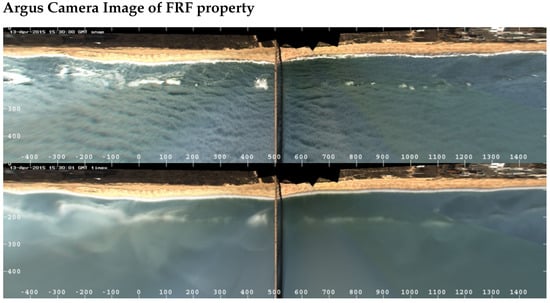
Figure 1.
Argus imagery products for 1530 13 April 2015. Images are rectified in a local coordinate system with distance along the coast on the x-axis and distance cross-shore on the y-axis. The top image is a snapshot image in which wave crests and instantaneous wave breaking are visible. The bottom image is a time-averaged (Timex) image for a 10 min period. Bands of white indicate wave breaking activity.
Successful bathymetric inversion at the FRF utilized the synthetic FCNN with remotely-sensed imagery from the Argus tower []. Figure 1 is an important step to a fully generalizable deep-learning-based depth inversion algorithm for the surf zone. This is the first time that FCNNs have been used to produce bathymetric measurements in the aerated and turbid waters typically found in the surf zone. Additionally, the inferences are at high resolutions—1 m in both the along-shore and cross-shore—and produced hourly (during daylight). This high-resolution output is necessary to capture the high variability of the surf-zone bottom boundary to be useful for a wide range of tasks. In particular, accurate bathymetries with greater temporal frequency would significantly improve bottom boundary conditions for wave and circulation modeling that utilize FRF observations [].
We begin the paper providing a brief overview of data sources in Section 2, and in Section 3, we detail our methodology and training data. Section 4 presents results, including overall model performance and comparison to eight survey-derived bathymetries. Section 5 discusses the results through example cases and provides a comparison to the instantaneous cBathy (Phase 2) output for these time periods. Section 6 discusses the implications of the fully convolutional neural network (FCNN) architecture, and Section 6 presents conclusions.
2. Data Sources
The primary data sources used in this study are (1) time-exposure (Timex) and snapshot (single video frame) image products, (2) bathymetric survey data, and (3) bulk wave statistics including wave height, period, and direction. In addition, we compare results to the cBathy linear depth inversion algorithm []. All measurements were collected at the U.S. Army Corps of Engineers Field Research Facility (FRF) in Duck, North Carolina.
The image products were collected from an Argus [] station, which consists of six cameras mounted on a 43 m observation tower. Images collected by the six cameras are merged and rectified to produce a combined 3 km (shore-parallel) by 0.5 km (shore-normal) field of view. The Timex images consist of an average of 700 video frames collected over a 10-min period. Both Timex and snapshot image products are available on a half-hourly basis.
Surveys are conducted at the FRF at approximately monthly intervals using the Coastal Research Amphibious Buggy (CRAB) or Lighter Amphibious Resupply Cargo (LARC). The data products collected with both vehicles have centimeter-scale vertical accuracy. Typically, surveys cover an approximately 1 km2 region that extends to an approximately 15 m depth. Along-shore survey transect spacing is nominally 43 m. Survey transect data are interpolated (using the interpolation method described in []) to create a high-resolution two-dimensional gridded bathymetry product.
The FRF 8 m array [] consists of 15 bottom-mounted pressure sensors. The array is located approximately 900 m from the shoreline. Data from the array are processed to produce directional wave spectra from which estimates of mean wave height, period, and direction are derived. Typically, these data products are available hourly.
cBathy is a linear depth inversion algorithm that infers bathymetry from nearshore video imagery []. The cBathy algorithm operates in three phases. In phase 1, cBathy calculates wavenumber-frequency pairs by identifying coherent patterns in cross-spectral analysis of image intensity time series. In the second phase, cBathy determines the depth that produces the best fit between phase 1 estimates of wavenumber and frequency and those modeled with the linear dispersion relation. Phase 2 additionally provides a self-diagnostic error metric. In Phase 3, a Kalman filter can be applied in time to provide more robust estimates of depth if hourly cBathy estimates are available. The internal error metric determined in phase 2 along with a site-specific process error are used to determine the Kalman gain.
Argus Timex and snapshot images and wave data are used as input to the ML network, and survey data are used to provide ground-truth data for training and testing. Details on the neural network and training/testing workflow are described in the following section. cBathy phase 2 estimates are used as baseline comparison data in the Discussion. Instantaneous cBathy phase 2 results are displayed, instead of the phase 3 Kalman-filtered product, in order to compare bathymetry estimates that depend only on data from the current time period for both methods.
3. Methodology
3.1. Neural Network Model
We use transfer learning for domain adaption with the FCNN developed in [] to develop the FCNN used in this effort. The model in [] was trained on synthetic Timex and snapshot imagery generated with the two-dimensional Boussinesq wave model Celeris [] over a variety of synthetic bathymetries and wave conditions. The original FCNN from [] (Figure 2) ingested a three-dimensional array of size (512, 512, 3). The first channel consisted of the red, green, blue (RGB) mean of a synthetic Timex image; the second channel used the RGB mean of a synthetic snapshot image; and the third channel included wave statistic information (i.e., wave height, wave period, wave direction). Values in the third channel were set to zero in cases when wave information was unavailable. The output of the model was a prediction of seabed elevation at the same resolution as the input Timex/snap pair.
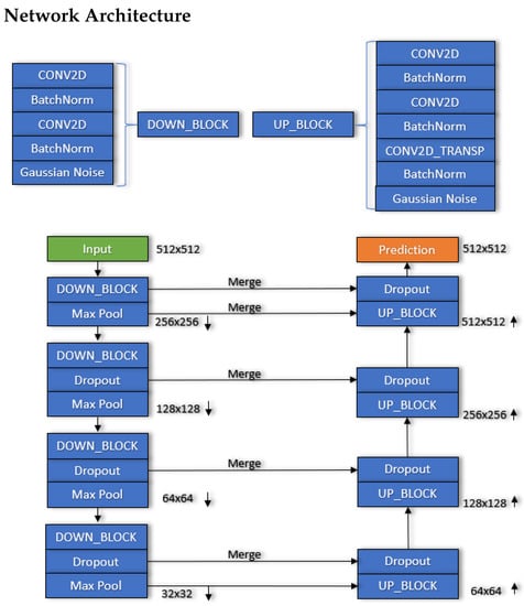
Figure 2.
A diagram of the network architecture used in this study. Down-sampling and up-sampling convolutional blocks are defined independently. Input data travel through a combination of down-sampling blocks, dropout, and pooling layers. The final down-sampled output is then passed through a combination of up-sampling blocks, dropout, and merge layers to create a final prediction of bathymetry. Figure from [].
3.2. Experiment Workflow
The model developed in [] was retrained to infer bathymetry at the FRF. The model was initialized with the weights from [], and Timex and snapshot imagery from the Argus tower were input in the first and second channels, respectively, in place of the synthetic imagery. Bulk wave statistics (significant wave height, dominant wave period, and mean wave direction) were used as additional input features to the model, when available, but are not required for the model to produce an output. Output (labels) associated with example input for the training and testing sessions were derived from FRF survey data.
The model was trained on data from 2015–2018 inclusive and tested on image-survey pairs from 2019. We considered images coincident to a survey if taken within three calendar days. The training set consisted of 41 survey-derived bathymetries and 3036 associated images, and the test set contained 11 survey-derived bathymetries and 306 associated images. While we used the full data input in the cross-shore, the model was only trained on the center one kilometer of the imagery (roughly +/−500 m from the tower) because this portion of the imagery contains the clearest imagery with the least projection artifacts. To create a final bathymetric estimate over the one-kilometer along-shore domain, we used a sliding window method, where the prediction window (500 m along-shore, 500 m cross-shore) starts at the northern end of the property and is shifted southward by 50 m to create another prediction, and so forth, until the entire along-shore property range has been predicted at least once. The mean of any overlapping predicted values is taken to produce a final inferred water depth value at each cell (between 50 and 500 values for each cell). The total time to read input, preprocess the data, and deliver a bathymetry estimate is approximately 5 min on a Windows laptop with an NVIDIA QUADRO RTX 4000 GPU. The required time scales linearly with additional inferences.
Images of questionable quality due to weather/time-of-day effects (i.e., fog, rain, and glare) and those recorded while cameras were not functioning properly were removed from both the training and testing sets. Additionally, to help overcome smaller lighting and weather effects that are present in even the highest quality data, a random pixel intensity change is applied at each sliding window step and predicted in a batch of size 100 to produce an ensemble of bathymetries that is then averaged to produce a final guess. Mini-batch normalization was used with a batch size of 8. The sigmoid activation function and mean absolute error loss returned the best results during preliminary hyperparameter investigation.
4. Results
Table 1 and Figure 3 quantify the overall results of testing the ML model. Overall pixel-wise RMSE is 0.37 m (Table 1) for the entire test set. RMSE was spatially variable with the lowest errors offshore of 300 m and slightly higher estimates closer to shore, between the sandbar and the shoreline (Figure 3b). There was also a region of higher error in Figure 3 that corresponds to the location of the FRF pier at ~500 m on the along-shore location (see Figure 1). When normalized by water depth, the highest percent errors occurred near the shoreline (near 40%), whereas the rest of the domain had errors on the order of 10 to 20% (Figure 3c). Over all test cases, model bias was low (0.06 m (Table 1). However, Figure 3d indicates clear spatial trends in bias: the model tended to overestimate depth closer to shore, between the shoreline and sandbar, and underestimated depths in the offshore region, particularly near the trough associated with the FRF pier (Figure 3d). The pixel-wise 1:1 map shows generally good agreement at the full range of depths between the predicted and surveyed depth (Figure 3e). Histograms of image-wise RMSE and bias are displayed in Figure 3f,g, respectively. In most cases, image-wise RMSE is less than 0.60 m. Mean image-wise depth bias is close to zero, with a slight shift towards over prediction of depths.

Table 1.
The depth bias, mean absolute error, RMSE (pixel-wise), and the 90th percentile error over the test set (Duck, NC 2019).
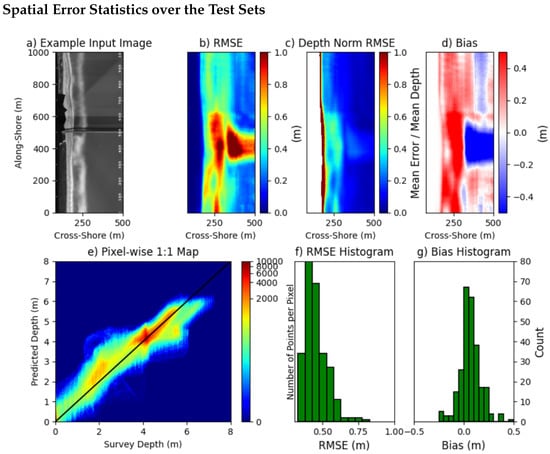
Figure 3.
(a) Example input Timex image, (b) Spatial RMSE, (c) depth-normalized RMSE, and (d) bias are shown as a function of cross-shore (x-axis) and along-shore (y-axis) coordinates over the entire test set. (e) shows a 1:1 plot of the surveyed depth to predicted depth for each cell, colored by the number of occurrences for each depth pair. Histograms of image-wise RMSE and bias are shown in (f,g), respectively. The shoreline in this figure, and all following figures, is vertically oriented to the FRF coordinate system, with increased distance from shore being shown on the x-axis.
Time series of predicted and surveyed two-dimensional bathymetry examples and transects are shown over the 2019 test set in Figure 4 and Figure 5. To evaluate the model under varying wave conditions, model performance was assessed relative to survey-derived bathymetry within three days of the imagery input. Wave conditions for each image are shown in Table 2 along with the time between the survey and image. The displayed transect corresponds to the FRF cross-shore array [] of wave gauges and was chosen because of its far location from the anomalous effects observed near the pier. The model produces realistic bathymetry estimates for all the test cases and correctly captures a range of surf-zone morphologies. These results include differing beach states with the morphology transitioning between single and double-barred systems over the course of 2019. In most cases, the model locates the sandbar position, but it sometimes fails to accurately estimate the sandbar amplitude. For example, the model correctly identifies the formation and offshore movement of an inner sandbar between February and April (Figure 4a,f,k,p). During this same time period, the model correctly places an outer sandbar near X = 400 m but overestimates its amplitude. In addition, the model correctly identifies the transition from a double-barred profile to a single-barred profile between November and December (Figure 5f,k,p) but again overestimates offshore sandbar amplitude in June and September (Figure 5a,f). The model fails to capture the deep trench under the FRF pier in all of these test cases, particularly south of the pier, which could possibly be explained by the pier obscuring wave signatures in this region. The variability in model performance over the test set is explored in the following section.
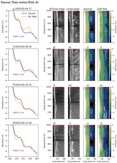
Figure 4.
Example model results for four dates in the first half of 2019. For each date, subplots (a,f,k,p) plot elevation versus cross-shore position for a transect at 940 m in the along-shore from the interpolated survey product (orange) and the model prediction (blue). Subplots (b,g,l,q) plot the input Timex image; subplots (c,h,m,r) plot the input snapshot image; subplots (d,i,n,s) plot the interpolated survey bathymetry; and subplots (e,j,o,t) plot the model prediction.
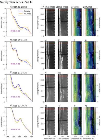
Figure 5.
Example model results for the four dates in the second half of 2019. (a–t) show the same information described in Figure 4 for the shown dates.
5. Discussion
5.1. Comparison to Optical Wave-Based Inversion Methods
The overall error shown over the test set of 0.37 m RMSE (Table 1, Figure 3), compares favorably relative to the scale of errors that typically occur from optical wave-based inversion methods within the surf zone. For example, prior work quantified the performance of cBathy phase 2 over a range of wave conditions, finding an RMSE between 0.51 and 0.89 m when wave heights were less than 1.2 m and between 1.75 and 2.43 m when wave heights were over 1.2 m []. In Figure 4 and Figure 5, we explore model performance in different conditions and compare the output of the ML network to both ground-truth and cBathy phase 2 estimates for the same time. cBathy also provides an error prediction at each cell, and cells with a predicted error of greater than 2 m are removed for this comparison. A Kalman filter could be applied to either product to potentially improve overall skill.
The first example is from transect four in Figure 5 on 10 December 2019. This example case is a single-barred system, with a break in the bar near the pier. The ML model performs well along both the transects at 60 and 940 m along-shore (Figure 6f) and captures the overall shape of the full two-dimensional survey product when comparing Figure 6b,c. The model predicts a break in the sandbar that is farther north than the survey product indicates. This is likely due to the corresponding gap in wave breaking in the Timex imagery at that location, between 400 and 500 in the along-shore. We observe good agreement at deeper depths between the model and the survey, and clear wave crests are visible throughout the snap imagery in this region (Figure 6e). cBathy provides relatively complete depth estimates at this time, though it has higher error throughout, translating the sandbar onshore through much of the northern portion of the domain (Figure 6i).
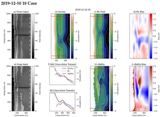
Figure 6.
Additional plots evaluating the bathymetry from the fourth row of Figure 5 and comparing to the cBathy phase 2 output for the same time period. (a) shows the Timex image input. (b) shows the “truth” bathymetry. (c) ML predictions. (d) shows the ML depth bias. (e) shows the snap image input. (f) shows two cross-shore transects at the 60 and 940 along-shore position for the survey and the ML/cBathy methods. (h) shows the cBathy prediction, and (i) shows the cBathy bias. Wave height (H = 0.98 m), period (T = 9.09 s), wave direction (D = 108°).
Figure 7 examines an example of some of the highest-error cases in the test set, when the network is biased deep throughout the nearshore area. In this case, the ML bathymetry estimate has a higher error close to shore than the cBathy results for the same time period. In this example, there is minimal wave breaking in the snap and Timex input, and the peak period is only 4.11 s. Correspondingly, the wave field in the snap image has low coherence. It is likely that the lack of visible wave breaking in the image, along with the scarcity of prominent wave crests in the snapshot image, provides insufficient information to accurately estimate depths or the position of the sandbar. In this case, the cBathy product is more accurate than the ML model close to shore, as wave parameters may be more readily distinguishable from noise in spectral analysis of the time-series data. In addition, cBathy can take advantage of multi-frequency waves in its results, whereas the ML inversion designed here can only interpret information from the visibly dominant wave in a single frame, which in this case is a very high frequency and thus less sensitive to depth.
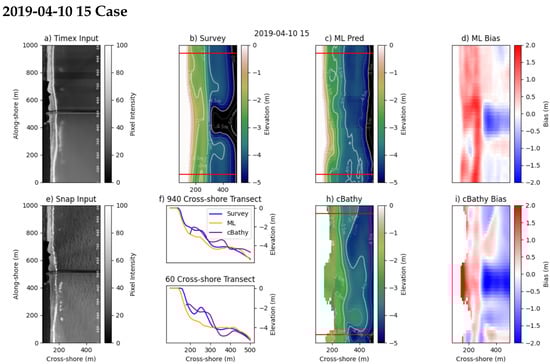
Figure 7.
Additional plots evaluating the bathymetry from the third row of Figure 4 and comparing to the cBathy phase 2 output for the same time period. (a) shows the Timex image input. (b) shows survey-derived bathymetry. (c) ML predictions. (d) shows the ML depth bias. (e) shows the snap image input. (f) shows two cross-shore transects at the 60 and 940 along-shore position for the survey and the ML/cBathy methods. (h) shows the cBathy prediction, and (i) shows the cBathy bias. Wave height (H = 0.57 m), period (T = 4.10 s), wave direction (D = 109°).
Figure 8 presents results from an image that occurs three days after the previous case (Figure 7). Both image results are evaluated with the same bathymetry. Unlike the previous case, longer period swell wave crests are clearly distinguishable in the snap image (Figure 8e), the dissipation signal is easily visible in the Timex image (Figure 8a), and bathymetry estimates from the ML model are more in the nearshore (Figure 8c). In contrast, cBathy, (Figure 8d,h,i), displays a more pronounced deep bias in this region of the domain.
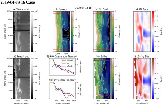
Figure 8.
Additional plots evaluating the bathymetry from the fourth row of Figure 4 and comparing to the cBathy phase 2 output for the same time period. (a) shows the Timex image input. (b) shows the “truth” bathymetry. (c) ML predictions. (d) shows the ML bias. (e) shows the snap image input. (f) shows a cross-shore transect at the 940 along-shore position for the survey and the ML/cBathy methods. (h) shows the cBathy prediction, and (i) shows the cBathy bias. Wave height (H = 1.21 m), period (T = 8.25 s), wave direction (D = 114°).
These results suggest that the model performs better when wave breaking is clearly visible in the Timex image and/or when wave crests are clearly visible in the snap images, illuminating the refraction patterns and changes in wavelengths.
5.2. Activation Maps
To explore the hypothesis that the visibility of wave crests in the snap image has a direct effect on the ability of the ML model to estimate depths, we examine activation maps within network layers. Activation maps display output values from a neural network layer as an image. Figure 9 shows the snapshot inputs for the two example cases from Figure 7 and Figure 8, along with the prediction, ground truth, and example activation maps for the northern portion of the domain. Similar to [], wave breaking and refraction patterns are visible in activation maps from some of the network layers, suggesting the model is using this information in its predictions. The snap image for 10 April has a less distinct wave field and breaking pattern, while the snap image for the 13 April case has more pronounced wave crests. These more pronounced wave crests are producing a stronger signal in the same activation maps (Figure 9h) than the shorter and harder-to-distinguish wave patterns from the earlier time period (Figure 9d). Qualitatively, improved model performance occurs when these images appear clearer to expert observation and are more similar to the images produced for the synthetic model training set in []. The enhanced ability of the model when there are clear and distinguishable wave refraction patterns mirrors the success criteria from other synthetic approaches and state-of-the-art satellite methods [,,,]. We hypothesize that the ML model is more successful at estimating water depths under these conditions of greater wave pattern coherence than in cases where visual artifacts or complicated sea states can hinder wave pattern identifications. Future work will endeavor to explore this hypothesis further.
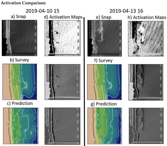
Figure 9.
Activation maps from a single ensemble window are shown for the northernmost section for the example shown in transects three and four in Figure 4 and detailed in Figure 7 and Figure 8. (a) shows the snap image for the labeled date. (b) shows the survey contours. (c) shows the instant prediction for that ensemble window. (d) shows three activation maps that emphasize the information that the network is keying off of to make its prediction. (e) shows the snap image for the labeled date. (f) shows the survey contours. (g) shows the instant prediction for that ensemble window. (h) shows three activation maps that emphasize the information that promotes a response in the network.
5.3. Wave Conditions
While wave-celerity-based inversions show degradation of results in high wave conditions [,,], the ML model performs similarly across different wave heights, periods, and directions. Figure 10 shows this invariance by comparing the absolute errors of each image in the test set with the offshore wave conditions recorded at the 8 m array during the image collection. Sample sizes across a wide range of wave periods (4–14 s) and directions (11–144°) show no correlation in mean error. For wave height, we see consistent mean error metrics (0.31 MAE, 0.37 RMSE) up to wave heights of 3.5 m. However, instances with high wave heights (>1.5 m) are more rare, and so more testing is needed to determine if estimates are similarly consistent under these conditions. Errors may slightly increase during small, short period waves, similar to Figure 7, when contrast on the front and back sides of the waves is low and little breaking occurs. Wave condition features were used as input during training/inference when available. Wave period was included, as it can affect wave speed in intermediate water depths and thus potentially interpretation of visible refraction patterns in the imagery. In addition, for a given bathymetry, variations in wave height will influence the extent of wave breaking visible in the Timex imagery. Interestingly, while including the local measured wave conditions did reduce the overall RMSE (0.369 m from 0.376 m), it was not statistically significant. More research is needed to determine if this is consistent across different locations.
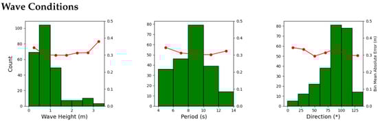
Figure 10.
Model error across different wave conditions. (a) shows the mean error versus the wave height. (b) shows the mean error versus the wave direction. (c) shows the mean error versus the wave period.
5.4. Transfer Learning
The network architecture utilized in [] provided a framework to explore the potential of transfer learning on FRF imagery and was able to incorporate some non-image features (wave height, period, and direction). Similar to [], activation maps for the real imagery used here highlight the wave breaking and refraction patterns in the imagery, suggesting the ML model is associating the visible signatures of shallow water wave processes with changes in water depth. This study demonstrates that an FCNN can accurately infer bathymetry using real-world Timex and snapshot imagery at the FRF, even with a training data set of limited size (3036 image/41 surveyed bathymetry pairs). More research is needed to determine the value of transfer learning from a network pretrained on physically realistic synthetic data. The transfer learning approach may add value when applying the network to locations with limited or no data availability. The applicability of the synthetic data to a general real-world location could possibly be enhanced by dimensional reduction of the synthetic and remotely sensed image pairs into a latent space. This would be expected to increase similarity and reduce environmental noise while retaining necessary information for the bathymetric inversion. The transfer learning component may be less important, however, for sites where large volumes of training data are available.
6. Conclusions
In this work, we explored the adaptation of an FCNN trained on synthetic surf-zone imagery [] to infer bathymetry from real Timex and snapshot imagery. This was the first time, to the authors’ knowledge, a neural network was successfully applied to infer bathymetry from remotely sensed sea-surface imagery in the surf zone. Not only did the approach provide accurate bathymetry estimates (RMSE = 0.37 m), but it also was effective with a relatively small training data set (3036 images/41 surveyed bathymetries). Additionally, all inferences over the test set predicted physically realistic bathymetric states. The model is robust to different wave conditions; however, estimates are most accurate when wave breaking and/or wave crests are clearly visible in imagery. Activation maps show that the model can learn the relationship between wave breaking signatures and underlying bathymetry, instead of merely overfitting to a mean bathymetric state. On the contrary, it accurately tracks patterns of morphologic change and infers transitional states between single-barred and double-barred profiles. Future work will be twofold: (a) developing a generalized form of the algorithm to work on wave fields from other locations, without requiring training data from those locations, and (b) examining the best approach to integrate this methodology into other bathymetric inversion methods and available data sources at the FRF, with the goal of developing the best bathymetry product possible on a daily time scale between survey dates.
Author Contributions
Conceptualization, A.M.C., M.P.G., T.J.H., A.S.B., K.L.B. and M.W.F.; Data curation, A.M.C.; Formal analysis, A.M.C., M.P.G., K.L.B. and M.W.F.; Funding acquisition, M.P.G., A.S.B. and K.L.B.; Investigation, A.M.C., T.J.H., K.L.B. and M.W.F.; Methodology, A.M.C., M.P.G., T.J.H., K.L.B. and M.W.F.; Project administration, M.P.G. and K.L.B.; Software, A.M.C.; Supervision, M.P.G., T.J.H., A.S.B., K.L.B. and M.W.F.; Validation, A.M.C.; Visualization, A.M.C.; Writing—original draft, A.M.C. and M.P.G.; Writing—review and editing, A.M.C., M.P.G., T.J.H., A.S.B., K.L.B. and M.W.F. All authors have read and agreed to the published version of the manuscript.
Funding
This research was funded by the U.S. Army Corps of Engineers Coastal and Ocean Data Systems Program and the Assistant Secretary of the Army for Acquisition, Logistics, and Technology [ASAALT] under 0603734/T08/11 and 0603463/AS9/02.
Acknowledgments
This research would not have been possible without the efforts of the world-class operations team at the Field Research Facility for their decades-long effort in placing and maintaining the instrumentation to collect wave data and the monthly bathymetric survey collections. We would like to thank the researchers that help to maintain and publicly serve the FRF’s coastal data including, but not limited to, Patrick Dickhudt, Kent Hathaway, Mike Forte, Jeff Gough, and Brittany Bruder. Additionally, we would like to extend thanks to Jonghyun Lee, Sourav Dutta, and Peter Rivera-Casillas for their expert consultation throughout the project.
Conflicts of Interest
The authors declare no conflict of interest.
References
- Wilson, G.W.; Özkan-Haller, H.T.; Holman, R.A. Data assimilation and bathymetric inversion in a two-dimensional horizontal surf zone model. J. Geophys. Res. Ocean. 2010, 115. [Google Scholar] [CrossRef]
- Plant, N.G.; Edwards, K.L.; Kaihatu, J.M.; Veeramony, J.; Hsu, L.; Holland, K.T. The effect of bathymetric filtering on nearshore process model results. Coast. Eng. 2009, 56, 484–493. [Google Scholar] [CrossRef]
- Sallenger, A.H., Jr.; Holman, R.A.; Birkemeier, W.A. Storm-induced response of a nearshore-bar system. Mar. Geol. 1985, 64, 237–257. [Google Scholar] [CrossRef]
- Holland, K.T.; Holman, R.A. Field observations of beach cusps and swash motions. Mar. Geol. 1996, 134, 77–93. [Google Scholar] [CrossRef]
- Birkemeier, W.A.; Mason, C. The CRAB: A unique nearshore surveying vehicle. J. Surv. Eng. 1984, 110, 1–7. [Google Scholar] [CrossRef]
- Fredsøe, J.; Deigaard, R. Mechanics of Coastal Sediment Transport; World Scientific: Singapore, 1992; Volume 3. [Google Scholar]
- Jackson, D.W.T.; Cooper, J.A.G.; Del Rio, L. Geological control of beach morphodynamic state. Mar. Geol. 2005, 216, 297–314. [Google Scholar] [CrossRef]
- Gao, J. Bathymetric mapping by means of remote sensing: Methods, accuracy and limitations. Prog. Phys. Geogr. 2009, 33, 103–116. [Google Scholar] [CrossRef]
- Holman, R.A.; Stanley, J. The history and technical capabilities of Argus. Coast. Eng. 2007, 54, 477–491. [Google Scholar] [CrossRef]
- Brodie, K.L.; Bruder, B.L.; Slocum, R.K.; Spore, N.J. Simultaneous Mapping of Coastal Topography and Bathymetry from a Lightweight Multicamera UAS. IEEE Trans. Geosci. Remote Sens. 2019, 57, 6844–6864. [Google Scholar] [CrossRef]
- Almar, R.; Bergsma, E.W.J.; Maisongrande, P.; de Almeida, L.P.M. Wave-derived coastal bathymetry from satellite video imagery: A showcase with Pleiades persistent mode. Remote Sens. Environ. 2019, 231, 111263. [Google Scholar] [CrossRef]
- Bergsma, E.W.J.; Almar, R.; Maisongrande, P. Radon-Augmented Sentinel-2 Satellite Imagery to Derive Wave-Patterns and Regional Bathymetry. Remote Sens. 2019, 11, 1918. [Google Scholar] [CrossRef] [Green Version]
- Vos, K.; Harley, M.D.; Splinter, K.D.; Simmons, J.A.; Turner, I.L. Sub-annual to multi-decadal shoreline variability from publicly available satellite imagery. Coast. Eng. 2019, 150, 160–174. [Google Scholar] [CrossRef]
- Legleiter, C.J.; Roberts, D.A.; Lawrence, R.L. Spectrally based remote sensing of river bathymetry. Earth Surf. Process. Landf. 2009, 34, 1039–1059. [Google Scholar] [CrossRef]
- Eugenio, F.; Marcello, J.; Martin, J. High-resolution maps of bathymetry and benthic habitats in shallow-water environments using multispectral remote sensing imagery. IEEE Trans. Geosci. Remote Sens. 2015, 53, 3539–3549. [Google Scholar] [CrossRef]
- Jagalingam, P.; Akshaya, B.J.; Hegde, A.V. Bathymetry mapping using Landsat 8 satellite imagery. Procedia Eng. 2015, 116, 560–566. [Google Scholar] [CrossRef] [Green Version]
- Pacheco, A.; Horta, J.; Loureiro, C.; Ferreira, Ó. Retrieval of nearshore bathymetry from Landsat 8 images: A tool for coastal monitoring in shallow waters. Remote Sens. Environ. 2015, 159, 102–116. [Google Scholar] [CrossRef] [Green Version]
- Jawak, S.D.; Vadlamani, S.S.; Luis, A.J. A Synoptic Review on Deriving Bathymetry Information Using Remote Sensing Technologies: Models, Methods and Comparisons. Adv. Remote Sens. 2015, 4, 147–162. [Google Scholar] [CrossRef] [Green Version]
- Jay, S.; Guillaume, M. Regularized estimation of bathymetry and water quality using hyperspectral remote sensing. Int. J. Remote Sens. 2016, 37, 263–289. [Google Scholar] [CrossRef]
- Lin, Y.C.; Cheng, Y.T.; Zhou, T.; Ravi, R.; Hasheminasab, S.M.; Flatt, J.E.; Troy, C.; Habib, A. Evaluation of UAV LiDAR for mapping coastal environments. Remote Sens. 2019, 11, 2893. [Google Scholar] [CrossRef] [Green Version]
- Vahtmäe, E.; Paavel, B.; Kutser, T. How much benthic information can be retrieved with hyperspectral sensor from the optically complex coastal waters? J. Appl. Remote Sens. 2020, 14, 16504. [Google Scholar] [CrossRef]
- Ashphaq, M.; Srivastava, P.K.; Mitra, D. Review of near-shore satellite derived bathymetry: Classification and account of five decades of coastal bathymetry research. J. Ocean. Eng. Sci. 2021. [Google Scholar] [CrossRef]
- Niroumand-Jadidi, M.; Vitti, A.; Lyzenga, D.R. Multiple Optimal Depth Predictors Analysis (MODPA) for river bathymetry: Findings from spectroradiometry, simulations, and satellite imagery. Remote Sens. Environ. 2018, 218, 132–147. [Google Scholar] [CrossRef]
- Niroumand-Jadidi, M.; Bovolo, F.; Bruzzone, L. SMART-SDB: Sample-specific multiple band ratio technique for satellite-derived bathymetry. Remote Sens. Environ. 2020, 251, 112091. [Google Scholar] [CrossRef]
- Patel, A.; Katiyar, S.K.; Prasad, V. Bathymetric Mapping of Bhopal City Lower Lake Using IRS-P6: LISS-4 Imagery and Artificial Neural Network Technique. J. Indian Soc. Remote Sens. 2016, 44, 605–616. [Google Scholar] [CrossRef]
- Wei, S.; Qian, J.; Yali, R.; Ran, M. Comparative Study of Different Machine Learning Models for Remote Sensing Bathymetry Inversion. In Proceedings of the International Conference on Intelligent and Fuzzy Systems, Istanbul, Turkey, 21–23 July 2020; Springer: Berlin/Heidelberg, Germany, 2020; pp. 1140–1148. [Google Scholar]
- Melsheimer, C.; Chin, L.S. Extracting bathymetry from multi-temporal SPOT images. In Proceedings of the 22nd Asian Conference on Remote Sensing, Singapore, 5–9 November 2001; Volume 9. [Google Scholar]
- Evagorou, E.; Mettas, C.; Agapiou, A.; Themistocleous, K.; Hadjimitsis, D. Bathymetric maps from multi-temporal analysis of Sentinel-2 data: The case study of Limassol, Cyprus. Adv. Geosci. 2019, 45, 397–407. [Google Scholar] [CrossRef] [Green Version]
- Sagawa, T.; Yamashita, Y.; Okumura, T.; Yamanokuchi, T. Satellite derived bathymetry using machine learning and multi-temporal satellite images. Remote Sens. 2019, 11, 1155. [Google Scholar] [CrossRef] [Green Version]
- Misra, A.; Ramakrishnan, B. Assessment of coastal geomorphological changes using multi-temporal Satellite-Derived Bathymetry. Cont. Shelf Res. 2020, 207, 104213. [Google Scholar] [CrossRef]
- Niroumand-Jadidi, M.; Bovolo, F.; Bruzzone, L.; Gege, P. Physics-based bathymetry and water quality retrieval using planetscope imagery: Impacts of 2020 COVID-19 lockdown and 2019 extreme flood in the Venice Lagoon. Remote Sens. 2020, 12, 2381. [Google Scholar] [CrossRef]
- Lippmann, T.C.; Holman, R.A. The spatial and temporal variability of sand bar morphology. J. Geophys. Res. Ocean. 1990, 95, 11575–11590. [Google Scholar] [CrossRef]
- Drusch, M.; Del Bello, U.; Carlier, S.; Colin, O.; Fernandez, V.; Gascon, F.; Hoersch, B.; Isola, C.; Laberinti, P.; Martimort, P.; et al. Sentinel-2: ESA’s Optical High-Resolution Mission for GMES Operational Services. Remote Sens. Environ. 2012, 120, 25–36. [Google Scholar] [CrossRef]
- Roy, D.P.; Wulder, M.A.; Loveland, T.R.; Woodcock, C.E.; Allen, R.G.; Anderson, M.C.; Helder, D.; Irons, J.R.; Johnson, D.M.; Kennedy, R.; et al. Landsat-8: Science and product vision for terrestrial global change research. Remote Sens. Environ. 2014, 145, 154–172. [Google Scholar] [CrossRef] [Green Version]
- Lippmann, T.C.; Holman, R.A. Quantification of sand bar morphology: A video technique based on wave dissipation. J. Geophys. Res. Ocean. 1989, 94, 995–1011. [Google Scholar] [CrossRef]
- Holland, K.T.; Holman, R.A.; Lippmann, T.C.; Stanley, J.; Plant, N. Practical use of video imagery in nearshore oceanographic field studies. IEEE J. Ocean. Eng. 1997, 22, 81–92. [Google Scholar] [CrossRef]
- Aarninkhof, S.G.J.; Holman, R.A. Monitoring the nearshore with video. Backscatter 1999, 10, 8–11. [Google Scholar]
- Aarninkhof, S.G.J.; Turner, I.L.; Dronkers, T.D.T.; Caljouw, M.; Nipius, L. A video-based technique for mapping intertidal beach bathymetry. Coast. Eng. 2003, 49, 275–289. [Google Scholar] [CrossRef]
- Aarninkhof, S.G.J. Nearshore Bathymetry Derived from Video Imagery. Ph.D. Thesis, Delft University, Delft, The Netherlands, 2003. [Google Scholar]
- Aarninkhof, S.G.J.; Ruessink, B.G.; Roelvink, J.A. Nearshore subtidal bathymetry from time-exposure video images. J. Geophys. Res. Ocean. 2005, 110. [Google Scholar] [CrossRef]
- Van Dongeren, A.; Plant, N.; Cohen, A.; Roelvink, D.; Haller, M.C.; Catalán, P. Beach Wizard: Nearshore bathymetry estimation through assimilation of model computations and remote observations. Coast. Eng. 2008, 55, 1016–1027. [Google Scholar] [CrossRef]
- Stockdon, H.F.; Holman, R.A. Estimation of wave phase speed and nearshore bathymetry from video imagery. J. Geophys. Res. Ocean. 2000, 105, 22015–22033. [Google Scholar] [CrossRef]
- Plant, N.G.; Holland, K.T.; Haller, M.C. Ocean wavenumber estimation from wave-resolving time series imagery. IEEE Trans. Geosci. Remote Sens. 2008, 46, 2644–2658. [Google Scholar] [CrossRef]
- Holman, R.; Plant, N.; Holland, T. cBathy: A robust algorithm for estimating nearshore bathymetry. J. Geophys. Res. Ocean. 2013, 118, 2595–2609. [Google Scholar] [CrossRef]
- Bergsma, E.W.J.; Almar, R. Video-based depth inversion techniques, a method comparison with synthetic cases. Coast. Eng. 2018, 138, 199–209. [Google Scholar] [CrossRef]
- Wilson, G.W.; Özkan-Haller, H.T.; Holman, R.A.; Haller, M.C.; Honegger, D.A.; Chickadel, C.C. Surf zone bathymetry and circulation predictions via data assimilation of remote sensing observations. J. Geophys. Res. 2014, 119, 1993–2016. [Google Scholar] [CrossRef] [Green Version]
- Brodie, K.L.; Palmsten, M.L.; Hesser, T.J.; Dickhudt, P.J.; Raubenheimer, B.; Ladner, H.; Elgar, S.J.C.E. Evaluation of video-based linear depth inversion performance and applications using altimeters and hydrographic surveys in a wide range of environmental conditions. Coast. Eng. 2018, 136, 147–160. [Google Scholar] [CrossRef] [Green Version]
- Bergsma, E.W.J.; Conley, D.C.; Davidson, M.A.; O’Hare, T.J.; Almar, R. Storm event to seasonal evolution of nearshore bathymetry derived from shore-based video imagery. Remote Sens. 2019, 11, 519. [Google Scholar] [CrossRef] [Green Version]
- Bak, A.S.; Brodie, K.L.; Hesser, T.J.; Smith, J.M. Applying dynamically updated nearshore bathymetry estimates to operational nearshore wave modeling. Coast. Eng. 2019, 145, 53–64. [Google Scholar]
- Mandlburger, G. Bathymetry from Active and Passive Airborne Remote Sensing—Looking Back and Ahead. 2017. Available online: https://phowo.ifp.uni-stuttgart.de/2017/PDF/23-Mandlburger-Abstract.pdf (accessed on 1 October 2021).
- Dickens, K.; Armstrong, A. Application of machine learning in satellite derived bathymetry and coastline detection. SMU Data Sci. Rev. 2019, 2, 4. [Google Scholar]
- Yunus, A.P.; Dou, J.; Song, X.; Avtar, R. Improved bathymetric mapping of coastal and lake environments using Sentinel-2 and Landsat-8 images. Sensors 2019, 19, 2788. [Google Scholar] [CrossRef] [Green Version]
- Wilson, B.; Kurian, N.C.; Singh, A.; Sethi, A. Satellite-Derived Bathymetry Using Deep Convolutional Neural Network. In Proceedings of the IGARSS 2020—2020 IEEE International Geoscience and Remote Sensing Symposium, Waikoloa, HI, USA, 19–24 July 2020; pp. 2280–2283. [Google Scholar]
- Ai, B.; Wen, Z.; Wang, Z.; Wang, R.; Su, D.; Li, C.; Yang, F. Convolutional neural network to retrieve water depth in marine shallow water area from remote sensing images. IEEE J. Sel. Top. Appl. Earth Obs. Remote Sens. 2020, 13, 2888–2898. [Google Scholar] [CrossRef]
- Lumban-Gaol, Y.A.; Ohori, K.A.; Peters, R.Y. Satellite-derived bathymetry using convolutional neural networks and multispectral sentinel-2 images. Int. Arch. Photogramm. Remote Sens. Spat. Inf. Sci. 2021, 43, 201–207. [Google Scholar] [CrossRef]
- Mandlburger, G.; Kölle, M.; Nübel, H.; Soergel, U. BathyNet: A Deep Neural Network for Water Depth Mapping from Multispectral Aerial Images. PFG—J. Photogramm. Remote. Sens. Geoinf. Sci. 2021, 1–19. [Google Scholar] [CrossRef]
- de Silva, A.; Mori, I.; Dusek, G.; Davis, J.; Pang, A. Automated rip current detection with region based convolutional neural networks. Coast. Eng. 2021, 166, 103859. [Google Scholar] [CrossRef]
- Buscombe, D.; Carini, R.J.; Harrison, S.R.; Chickadel, C.C.; Warrick, J.A. Optical wave gauging using deep neural networks. Coast. Eng. 2020, 155, 103593. [Google Scholar] [CrossRef]
- Buscombe, D.; Ritchie, A.C. Landscape classification with deep neural networks. Geosciences 2018, 8, 244. [Google Scholar] [CrossRef] [Green Version]
- Ellenson, A.; Simmons, J.; Wilson, G.; Hesser, T.; Splinter, K.D. Machine Learning Classification of Beach State from Argus Imagery. Coast. Eng. Proc. 2020, 37. [Google Scholar] [CrossRef]
- Benshila, R.; Thoumyre, G.; Najar, M.A.; Abessolo, G.; Almar, R. A Deep Learning Approach for Estimation of the Nearshore Bathymetry A Deep Learning Approach for Estimation of the Nearshore. J. Coast. Res. 2020, 95, 1011–1015. [Google Scholar] [CrossRef]
- Collins, A.; Brodie, K.L.; Bak, S.; Hesser, T.; Farthing, M.W.; Gamble, D.W.; Long, J.W. A 2D Fully Convolutional Neural Network for Nearshore and Surf-Zone Bathymetry Inversion from Synthetic Imagery of Surf-Zone using the Model Celeris. In Proceedings of the AAAI Spring Symposium: MLPS, Stanford, CA, USA, 23–25 March 2020. [Google Scholar]
- Collins, A.M.; Brodie, K.L.; Bak, A.S.; Hesser, T.J.; Farthing, M.W.; Lee, J.; Long, J.W. Bathymetric Inversion and Uncertainty Estimation from Synthetic Surf-Zone Imagery with Machine Learning. J. Remote. Sens. 2020, 12, 3364. [Google Scholar] [CrossRef]
- Al Najar, M.; Thoumyre, G.; Bergsma, E.W.J.; Almar, R.; Benshila, R.; Wilson, D.G. Satellite derived bathymetry using deep learning. Mach. Learn. 2021, 1–24. [Google Scholar] [CrossRef]
- Tavakkol, S.; Lynett, P. Celeris: A GPU-accelerated open source software with a Boussinesq-type wave solver for real-time interactive simulation and visualization. Comput. Phys. Commun. 2017, 217, 117–127. [Google Scholar] [CrossRef] [Green Version]
- Long, C.E.; Oltman-Shay, J.M. Directional Characteristics of Waves in Shallow Water (No. CERC-TR-91-1); Coastal Engineering Research Center: Vicksburg, MS, USA, 1991. [Google Scholar]
- Splinter, K.D.; Holman, R.A. Bathymetry estimation from single-frame images of nearshore waves. IEEE Trans. Geosci. Remote Sens. 2009, 47, 3151–3160. [Google Scholar] [CrossRef] [Green Version]
Publisher’s Note: MDPI stays neutral with regard to jurisdictional claims in published maps and institutional affiliations. |
© 2021 by the authors. Licensee MDPI, Basel, Switzerland. This article is an open access article distributed under the terms and conditions of the Creative Commons Attribution (CC BY) license (https://creativecommons.org/licenses/by/4.0/).