
Microgrid Protection through Adaptive Overcurrent Relay Coordination


Department of Computer Science and Electrical Engineering, University of Maryland Baltimore County, Baltimore, MD 21250, USA
*
Author to whom correspondence should be addressed.
Electricity 2021, 2(4), 524-553; https://doi.org/10.3390/electricity2040031
Submission received: 16 August 2021
/
Revised: 22 September 2021
/
Accepted: 1 November 2021
/
Published: 5 November 2021
Abstract
:The inclusion of distributed energy resources (DER) in Microgrids (MGs) comes at the expense of increased changes in current direction and magnitude. In the autonomous mode of MG operation, the penetration of synchronous distributed generators (DGs) induces lower short circuit current than when the MG operates in the grid-connected mode. Such behavior impacts the overcurrent relays and makes the protection coordination difficult. This paper introduces a novel adaptive protection system that includes two phases to handle the influence of fault current variations and enable the MG to sustain its operation. The first phase optimizes the power flow by minimizing the generators’ active power loss while considering tolerable disturbances. For intolerable cases, the second phase opts to contain the effect of disturbance within a specific area, whose boundary is determined through correlation between primary/backup relay pairs. A directional overcurrent relay (DOCR) coordination optimization is formulated as a nonlinear program for minimizing the operating time of the relays within the contained area. Validation is carried out through the simulation of the IEEE 9, IEEE 14, and IEEE 15 bus systems as an autonomous MG. The simulation results demonstrate the effectiveness of our proposed protection system and its superiority to a competing approach in the literature.
1. Introduction
The rising demand for uninterrupted power supply and the rapid growth of infrastructure have motivated the introduction of MGs. An MG corresponds to DER and loads that can be managed in an efficient manner. An MG can be connected to the main grid or operate in an autonomous mode [1].
Sustaining MG Stability: While MGs enable integrating DER into traditional distribution networks, protection against fault remains as one of the critical challenges for successful MG operation. The majority of the existing protection techniques target radial distribution networks [2,3,4]. In the presence of DER, these techniques will not be directly applicable to MGs because DER introduces dynamic behaviors that disturb the electrical components and consequently cause a serious threat to MG stability [5]. Protective relays are one of the key electrical components that detect faulty equipment. They, in essence, allow isolation of the faulty part to prevent cascaded failure throughout the grid [6].
Faults occur in MG due to sudden operational changes and environmental events. A fault causes disturbance in the power flow balance and triggers an emergency state that requires immediate response to properly detect and isolate the fault. In a traditional distribution grid without DG, static settings of OCRs suffice. However, in the presence of DER, OCRs will experience challenging changes in the power flow direction and fault current level. The first challenge can be addressed by DOCRs. However, the second cannot be easily resolved because the DER will cause significant fluctuation in total overcurrent during faults [6]. Specifically, in the presence of DER fault current introduces several issues; inconsistent activation of DOCRs is the prime among these issues. In any protection system there are primary and backup relays, which operate in a coordinated manner with latency between their activation, called Coordination Time Interval (CTI). When many relays are employed, static coordination becomes quite complex, and relays may fail to react due to overcurrent fluctuation. Hence, a proper adaptive DOCR coordination is necessary for MG operation, where the DOCRs adjust their settings to cope with variations in the fault current.
Issues with Existing MG Protection Strategies: Existing protection strategies deal with fault overcurrent in MG through either: (i) limiting DG capacities; (ii) inserting external devices; or (iii) applying coordinated activation of protection devices to isolate the fault. A technique pursuing the first strategy opts to mitigate the effect of faults by determining the optimal location and capacity of DERs such that their contributions during the fault are insufficient to impact the relay operation. However, disconnecting DGs for temporary faults leads to voltage dip and causes instability [7,8]. The second strategy relies on inserting external devices to the MG. A popular example of these devices is the fault current limiter (FCL). FCL reduces fault currents to a level that enables the use of protective devices. However, FCL imposes large impedance and consequently degrades the system transient and voltage stability. Finally, the third strategy relies on employing protection devices that can cooperatively clear the fault by separating areas containing disturbances from the rest of the MG. The protection scheme can be voltage-based protection, differential protection, and distance protection. None of the existing schemes that pursue this strategy leverages communication links in orchestrating the fault response; therefore, they are not flexible and do not adapt to varying MG conditions. Our proposed mechanism follows the same strategy and overcomes the aforementioned shortcoming. More details on existing protection schemes in this category will be provided in Section 2.
Contribution: This paper presents an effective protection mechanism that copes with the dynamic nature of MGs. The proposed mechanism can handle both tolerable and intolerable disturbances. It mitigates the influence of fault current level fluctuation on DOCRs by applying two phases of optimizations. The first phase deals with instability in the MG by applying optimal power flow (OPF) to increase the reliability in the MG. The OPF aims to minimize generators active power loss while tolerating the operating points of the MG to achieve system stability. However, in severe situations, it is difficult to deal with major disturbances through OPF. Therefore, the second phase tackles unbearable disturbances, such as line failures that cause fault current variations. In this phase, we introduce a novel strategy to contain the failure within a specific zone and identify the impacted relays. The determination of the fault containment zone and the impacted relays is based on the primary/backup relay pair correlation. Once the boundaries of the affected zone are detected, our mechanism readjusts the relay settings only in the containment zone. We mathematically formulate the optimal overcurrent relays coordination problem as a nonlinear program. The key advantages of our mechanism are that it rapidly contains the spread of failure by resetting the fewest relays and boosts the MG stability through power flow optimization. The validation results using MGs based on the IEEE 9, IEEE 14, and IEEE 15 bus systems, confirm these advantages. The contributions of this paper can be summarized as follows:
- We propose a protection mechanism that handles the two types of disturbances caused by the fault current variations.
- We develop a new technique to identify the MG mode of operation using the DG measurements from the power flow analysis, without reliance on communication with the main feeder.
- We introduce a novel MG protection strategy based on the correlation of primary/backup relay pairs. The approach identifies the impacted area with the minimum number of relays to be readjusted.
- We mathematically formulate the overcurrent relay coordination problem; the optimization is accurately identifying the boundaries of a fault containment zone with the least number of relays involved in.
The organization of the rest of this paper is as follows. Section 2 discusses related work in the literature. Section 3 states the system assumptions and covers some preliminaries. In Section 4, our proposed MG protection system is described in detail. The simulation results are presented in Section 5. Finally, the paper is concluded in Section 6. Definitions of key concepts are provided in Appendix A for quick reference. Additional validation results are included in Appendix B as well.
2. Related Work
Dynamic fluctuation of fault current is one the prominent issues introduced by the penetration of DER in MGs. As mentioned earlier, our approach strives to isolate the fault through the coordinated activation of relays. The focus in this section is on schemes that exploit protective relays.
2.1. Distance-Based Protection
Multiple schemes have pursued such a distance-based protection to make tripping decisions on activating relays in MG [9,10]. Essentially, the main problem in using the distance protection is that the DER between the measurement point and fault point acts as an intermediate in-feed that is negatively affecting the accuracy of impedance measurement. In fact, distance protection is more applicable for the protection of transmission grids [11]. Their consideration for applications in MG is still difficult [12].
2.2. Differential Protection
There are two categories of work on differential protection. The first category involves a central controller based on the data received from the monitoring relays [13,14]. None of the existing schemes have factored in the delay due to conducting the data analysis before the protective action is taken. Therefore, the primary protection may not work properly. The second category of work pursues a distributed control methodology. Accordingly, each relay communicates individually with its adjacent relays and observes the direction of the current. Several papers used multi-agent based differential protection [15,16]. Yet, the main issue with multi-agent systems is the computational complexity, which limits scalability for large MGs.
2.3. Overcurrent Protection
Overcurrent protection is commonly used for conventional distribution systems due to its low cost and ease of deployment. This type of protection requires some modifications so that it can be utilized for mesh-connected MG with DERs. In an autonomous mode of MG operation, the fault current level is reduced, and accordingly long tripping time is required to detect faults [17]. In such a case, the protection scheme becomes uncoordinated. Several studies have been conducted to overcome such a challenge. Jones et al. [18] have tackled the deficiency of faulty current identification using electromechanical and digital overcurrent relays that are equipped with directional components and have only a single setting. In addition to its high cost, this approach considers only synchronous DGs, i.e., those whose frequency matches that of the grid. In [19,20], a dual setting DOCR is introduced to minimize the total operating time of primary/backup relay pairs; every relay has two settings to handle the bidirectional fault currents. While the dual setting reduces the relay’s operating time, the relay design becomes complicated and boosts the cost of fault protection in MGs.
2.4. Adaptive and Pre-Planned Protection
The aforementioned protection schemes can be further classified as pre-planned and adaptive. The former is based on an offline analysis to determine a set of relay settings applicable under specific fault scenarios. Such offline analyses are conducted at the time of MG setup or relay deployment. No communication links are exploited for coordination [21]. On other hand, adaptive protection schemes analyze the fault scenario in real-time and determine the response in accordance with the grid conditions. In this paper, we advocate adaptive overcurrent protection. Generally, an adaptive protection system involves a group of digital relays, an intelligent control system that observes and responds to the grid events, as well as communication infrastructure to transfer data. The settings of the relays are dynamically readjusted whenever changes occur during MG operation. Ustun et al. [22] proposed a scheme that readjusts the relay settings based on the MG topology. However, only the main grid utility and contingencies of DGs are considered; the transmission lines contingency is not factored in. Failure of any electrical components during operation severs grid connectivity. The adaptive protection system of [23] solves the coordination problem by minimizing the operating time of all primary relays in the MG. Yet, they did not consider the small disturbances that the MG is susceptible to.
To the best of our knowledge, none of the protection approaches factor in minor and major disturbances. We have validated our protection system under various circumstances, load variation, line failures, and multiple independent line failures. In addition, our proposed system reduces the number of DOCRs involved in the fault isolation and can thus scale for large MGs. The proposed protection is quite practical and effective, as it does not require any external electrical devices or need of additional relay functionality. Table 1 provides a summary of the different protection strategies that address fault current variations.
3. System Model and Preliminaries
This section discusses the system model, assumptions, and provides some preliminaries.
3.1. Microgrid System Model
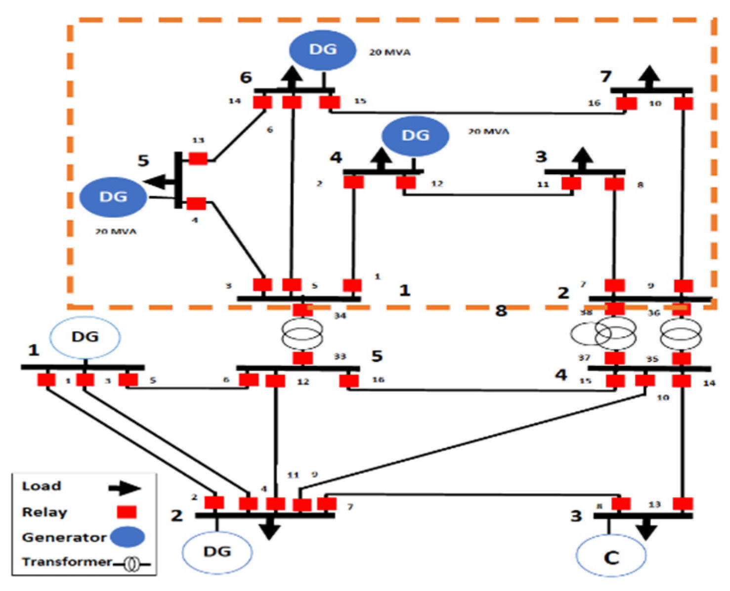
A microgrid is a relatively small part of the power distribution system that includes one or multiple distributed generation units and loads. An MG can operate while connected to the main grid (Grid-connected mode) and after getting separated from the main power network (Autonomous mode). The MG is often equipped with a set of protective devices, specifically, relays and circuit breakers, to mitigate the risk of unexpected dynamic events such as fault current fluctuation, bidirectional power flow, resynchronization of DGs, and false tripping. Figure 1 presents an example of an MG based on IEEE 14, which consists of 14 buses, 16 lines (circled numbers), 3 transformers, and 39 overcurrent relays (denoted as small squares). The IEEE 14 bus system is selected in this paper as an illustrative example because of its topological features and wide variety of components. The MG in Figure 1 is connected to the transmission network via two transformers. The DGs are located on buses 6 and 8. Protective relays are placed on all lines and typically follow the IEC standard [24]. CTI is a certain time interval that must be maintained between the primary and backup protective relays to ensure correct sequential operation. The time dial setting (TDS) is a means for adjusting the time for a relay to trip once the current exceeds the set value. Both CTI and TDS are considered in our optimization.
3.1.1. Power Source
During the islanded mode of operation, not all energy resources are capable of regulating the network voltage and frequency shedding [25]. Generally, energy sources in a microgrid are classified into two categories: dispatchable and non-dispatchable generators [26]. In this paper we are considering only the dispatchable generators that have the ability to adjust its power supply by controlling the voltage and frequency. Dispatchable generators are associated with a power electronic converter, which act as a synchronous machine [27]. The active power generation of this type of energy source is determined as:
where is the total active load power, is the droop coefficient for generator j, and Cg corresponds to the total power generation capacity.
3.1.2. Transmission Lines
The impedance parameters of transmission lines have great effect on grid operations, such as transient stability and state estimation, and are used as the basis for protective relay settings. We consider short transmission lines where the length is below 50 miles [28]. For such a category of lines, the parameters are lumped. Thus, the transmission line series impedance is a combination of the resistance and inductance together. Furthermore, the line capacitance is negligible and hence the admittance can be ignored. The short transmission line voltage and current equations are defined by:
where ρ is the resistance, is the inductive reactance, and are the voltage at the sending and receiving ends of the transmission line. Similarly, and reflect the current of sending and receiving ends of a transmission line.
3.1.3. Load Model
Loads can be classified into two types, namely, static and dynamic. We consider dynamic loads to be more practical for MG and the system exposed to disturbances that can be tolerable or problematic. Therefore, such dynamic load variation motivates the need for protective measures. In this study, we adopt the dynamic active and reactive power load of [29], which can be mathematically expression as follows:
where are the nominal values of the voltage, active power and reactive power at the load, respectively. Meanwhile, and are state variables related to active and reactive power dynamics. Finally, and are exponents related to the transient load response.
3.2. Protection System Model
The penetration of DERs contributes to internment fault current levels, and thus could impact the power distribution continuity and disrupt the coordination between protective devices. Such dynamic behavior constitutes a major challenge in protecting the MG. Therefore, it is crucial to employ an adaptive protection system. Our proposed adaptive protection system involves a MG central controller (MGCC) that communicates with every relay and DG in the MG over the standard IEC 61,850 connections. Figure 2 shows sample communication architecture.
Communication with relays is essential to update their operating currents, and hence isolate the fault properly. On the other hand, the DGs and main grid are monitored to check their status and their fault current contributions, i.e., whether the DGs are active or inactive (e.g., ON/OFF), and whether the MG is operating in islanded or grid connected. With these inputs, the MGCC estimates the tripping current value for each relay. In other words, the MGCC assigns the current value for which the relay should interrupt the connection. For a given relay in the MG, the operating current is calculated using (6), which considers the grids and DGs’ fault contribution on that particular relay:
where is the fault current contributed by the main grid; it is calculated using the Thévenin theorem, as:
with and being the Thévenin equivalents for the grid utility, impedance between the utility grid and point of calculation, respectively. In practice, varies with respect to distance. Hence, the equation of fault current contributed by the main grid becomes a function of distance (), , where is the distance from the main grid to the fault location. Meanwhile, represents the mode of operation; for an islanded mode = 0 and = 1 when the grid is in the connected mode. D is the number of distributed generators in the MG, is the fault current contributed by the DG, which can be approximated for the machine rotor to be 5 times its rated operating current [30], i.e., . is the DG operation status, with 0 and 1 reflecting inactive and active operation status, respectively.
denotes the impact factor of the nth distributed generator; it is introduced to calculate the fault contribution of DGs at distant points in the MG. It represents the decrease in the fault current due to inductance and resistance of LV distribution lines. is mainly dependent on the transmission line characteristics and the distance and can be expressed as ratio of the to , where is a DG’s fault current contribution at a distance point which is actually known before fault occurs. allows the MGCC to calculate all fault contributions and assign tripping current levels to the relays for proper operation. The fault current contribution can be expressed as where is the rated output voltage of DG based on the grid code. is the impedance of the transmission line per length, and is the distance between DG and the relay under consideration. The value of varies from 0 to 1, where relays closer to the DG under consideration will have a higher DG impact factor whereas those which are far will have a lower DG impact factor.
4. Microgrid Protection System
The main goal of any protection in a power system is to rapidly isolate the zones that contain disturbances while keeping the rest of the system operational. Due to DER, an MG usually suffers from an uncertain pattern of disturbances. Any disturbance, either limited or major, can affect the operation of the MG system [31]. Our proposed protection system is designed to be adaptive to the scope and impact of disturbance. All information required for protection is performed inside the MGCC. The MGCC collects measurements from DGs and relays and adjusts the power flow to satisfy the demand and maintain a tolerable MG operation under the effect of small disturbance. In case of major disturbance, the protection system contains the failure through the coordination of overcurrent relays. Before providing the detailed explanation of the methodology and steps, the next subsection gives an overview of the steps.
4.1. Approach Overview
Figure 3 provides a flowchart summary of the proposed protection system. It starts with power flow analysis to measure the new operating points. Our protection system determines the MG mode of operation via the calculated measurements from the power flow analysis; it distinguishes the mode of operation through the status of DGs active and reactive power. As shown in the figure, our approach operates in two phases. The first phase attempts to handle limited disturbances by maintaining the stability of the grid through optimal power flow (OPF). It makes appropriate changes in the load and power generation level to balance supply and demand in an MG. This can be done by activating spare DERs if any are available, or by increasing the generation rate for the already-engaged ones. The aim of the power flow optimization is to minimize the active power loss while sustaining tolerable operating points and a stable MG network [32,33,34]. The second phase deals with severe circumstances where the DGs bring major disturbance that can trigger outages [35]. The second phase aims to prevent the failure from spreading by readjusting the relay settings of the affected part of the MG, which we refer to as “Containment Zone”. In essence, the second phase deals with the overcurrent relay coordination problem and formulates it as a nonlinear program. The following describes the execution flow and is also articulated in Figure 3.
Once a disturbance occurs in the MG our proposed protection system is applied, to respond to any of the disturbances, the MGCC uses the power flow equations to identify the dynamic behaviors in the MG through the calculation of new operating points and assessing the status of the MG operation.
In case of load variation, which is a tolerable event (small disturbance), the optimal power flow (OPF) is performed to maintain acceptable load variation. OPF strives to increase the power generation capacity to handle the demand by minimizing the active power losses. In any power grid, the generation capacity must always exceed the load to allow for normal demand fluctuations. A suitable rule is to sustain online generation capacity at 120 percent of the steady state load [36].
Severe scenarios reflect major disturbance and correspond to when the penetrated DGs induced changes in the fault current by ±5% of its nominal value [37]. Such a major disturbance could cause the disconnection of transmission lines or DGs, and consequently would activate DOCRs. To alleviate the major disturbance, the second phase implements a new strategy to determine the boundaries of containment zones based on the coordination time interval of the primary/backup relay pairs and conducts optimal overcurrent relay coordination for only relays within the containment zone.
As mentioned above, our protection system performs power flow analysis at the first stage of the protection to determine the new operating points for dealing with disturbances and mitigating the risk of unstable operation. For that, the AC power flow analysis method is adopted from [38]. The balance of this section focuses on the remaining steps.
4.2. Identifying MG Mode of Operation
Recognizing the MG mode of operation is very important for protection because the MG system behaves differently in each mode. Appropriate protection systems should adapt to the operation mode. Generally, the mode of operation can be inferred using islanding detection techniques, which can be further classified as remote and local [39]. Remote techniques are based on the communication between utilities and DGs, where a SCADA system can determine whether the MG is islanded or not. On the other hand, local techniques interact directly with the grid operation by introducing perturbations or by monitoring some of the system parameters [40]. Our protection system employs local technique to identify the mode of operation using the measured active and reactive powers at each DG assists in determining the mode of operation. In the connected mode, the distributed sources supply constant active and reactive power because the main feeder supports the MG. On other hand, during the islanded mode of operation, when the main grid source is not present, the distributed sources are responsible for fulfilling the load demands. The active and reactive powers supplied by several distributed resources are not constant and normally variable. Therefore, the active and reactive power measurements from the power flow analysis are used as indicators to infer the mode of operation and determine protective action accordingly. The transition between the modes of operation can be detected by the DGs operating points [41]. Table 2 summarizes the categorization of the MG mode.
4.3. Power Flow Optimization (Phase I)
The MG operation is highly dynamic in nature. Nonetheless, all electrical components should operate within certain specific limits. If the generators surpass its rated value, it introduces unbalanced power flow that could cause MG instability. Adjusting the load and generated power would be necessary to cope with instability in the MG. The OPF procedure attempts to optimally do such adjustment by satisfying the power flow balance equations and constraints. Hence, the objective function is to minimize active power loss. The OPF is formulated as follows:
where is the active power loss, M is the number of buses, is the conductance of the line, and are the voltages at bus i and j, respectively, and and are the phase angle of voltage at the ith and the jth bus, respectively.
The objective function of (8) is subject to the following constraints:
Power flow balance
Observing the generator’s active and reactive power limits.
Keeping the voltages at the generators and load buses within acceptable limits.
The tap settings maintain an appropriate magnetic flux level in the transformer to provide the transformers nominal secondary output voltage. Hence, we must ensure that the ranges of the transformer tap settings are bounded
The OPF formulation is a nonlinear program and effectively determines the current injected to the MG by each DG. It seeks to find the optimal profile of active/reactive power at the generators; voltage magnitude of generators/load, and the transformer tap settings to minimize the active power loss, while satisfying the physical and operational constraints. Constraint (9) is for power flow balance, while constraints (10) and (11) are essential to make sure that the power is supplied to all loads in the MG. It ensures the robust system operation while keeping the active/reactive power of the generators within the upper and lower limits. When the load increases above the rated power output of the generators, power imbalance takes place-causing disturbance in the MG operation. At any point in time, the MG should sustain tolerable voltages on generator/load buses during steady state operating conditions, as reflected in (12) and (13). Too high or too low voltages could cause problems on the load buses. Consequently, the customer electrical devices would break down and cause system instability. Constraint (14) reflects the tap settings of the transformer. The transformer tap setting must adapt with various operating scenarios of the network to sustain proper voltage. Basically, the tap setting controls the voltage and current where the current is inversely proportional to both voltage and number of windings turns. This means if voltage grows, the current must be lowered and vice versa. In MGs, it is essential to change the transformer taps frequently within a limit to control the current.
4.4. Containment Zone Determination (Phase II)
To sustain the MG stability, the protection system should be responsive in activating the necessary measures. Therefore, our proposed relay coordination approach aims to minimize the number of re-adjusted relay settings in response to a fault by defining the impacted area, which we refer to as the containment zone. The relay coordination is a sequence of relay operations to handle possible fault location in the MG. Generally, the protective relays can be divided into two categories: primary and backup relays. A primary relay is the first defense with settings such that the fault clearing time is always less than the backup relay. The backup relay ensures fault handling if the primary relay fails to operate. The important requirement for the backup relays is to operate with sufficient time delay.
Our strategy is to define the containment zone boundaries and the relays involved in the zone. To do so, we rely on the primary/backup relay pair association. The operating time of the nearest relays to the faulted line is assessed to decide on their involvement in the coordination process. If the operating time of a relay is greater than zero, the operating time of the following backup relays must be measured considering the time gap reduction, which is essentially the CTI. The same steps are repeated sequentially until the operating time gets close to zero. As we move outward from the faulted line, the operating time of the backup relays decreases, and the relaying action eventually seizes. Any relay with operating time of zero or less will not be involved in the fault mitigation process. Recall that the operating time is relative to the primary and can thus be negative if the backup is faster in tripping.
Figure 4 presents the new strategy of determining the boundaries of the containment zone on a single line diagram of 8 transmission lines and 16 relays. The CTI is 0.2 s. It is assumed that the measured operating time of relays located on the faulted line is 0.32 s and all senses the fault simultaneously.
If a fault occurs in a line between buses 2 and 3, the operating time, top, of relays R3 and R4 during the fault is equal to 0.32 s; the corresponding backup relays are R6, R11, R14 R1, and R10. The operating time based on the coordination correlation of primary/backup relays is calculated as follows:
top(R6) = top(R11) = top(R14) = top(R1) = top(R10) =
top(faulted line) − CTI = 0.32 − 0.2 = 0.12 s
Since it is greater than zero, we have to check the following backup relays, namely, R8, and R16 whose is operating time is:
top(R8) = top(R16) = 0.12 − CTI = 0.12 − 0.2 = − 0.08 s
The value of top for R8, and R16 is not greater than zero; those relays do not have to be involved in the coordination process. Therefore, the containment zone includes relays around the fault with operating time greater than zero, namely R6, R11, R14, R1, and R10. Meanwhile, R8, and R16 remain unaffected by the fault.
4.5. Relay Coordination Optimization (Phase II)
4.5.1. DOCR Operating Time Formulation
An adaptive overcurrent relay’s operating time is a function that has an inverse relationship with the short-circuit current ( passing through relay (r) on faulted line (f) and a direct relationship with Time Dial Settings () as given below:
where is that plug setting and is referred to as the ratio of fault current in the OCR to its pickup current. is the pickup current and is calculated from the minimum value of fault current at which the OCR starts to operate. Based on acceptable IEC standards for inverse-time type, δ, and L are constants and taken as 0.14, 0.02 and 0, respectively.
Objective Function
The relay coordination problem is formulated as a nonlinear program; the main aim is to minimize the operating times of all relays within the identified containment zone while meeting the conditions of relay coordination.
where f refers to the fault, r is a relay, M is the total number of relays within the containment zone, is the operating time of a primary relay, b is the backup relay and N is the total number of backup relays for each primary relay within the containment zone, and ( is the operating time of backup relay. It is worth mentioning that the summation in (16) can be further aggregated over all simultaneous faults as long as they are independent and their corresponding containment zones do not overlap. In the future we plan to extend the scope to consider dependent, e.g., cascaded, failures where relay settings could be conflicting or synergetic.
Constraints
The relay coordination problem considered two types of constraints: (i) on relay characteristics, which limit the relay operating time, time dial setting and relay pick up current, and (ii) on the coordination of primary and backup relays. First, the Time Dial Setting (TDS) of each relay r should be bounded:
where and are the minimum and maximum TDS of the relay r, respectively. Typically, they are 0.05 and 1, respectively. On the other hand, observing the pickup current bounds prevents overreaction and lack of reaction:
Although it is desired for a relay to operate rapidly in order to prevent fault propagation, there are bounds imposed by the relay design that need to be taken into account while coordinating the DOCRs. A relay needs to have a particular minimum and maximum response time and , respectively. Hence, we can set up the values within that range.
To ensure adequate coordination between DOCRs, the response time of the backup relay should be equal or greater than the sum of the response times of its corresponding primary relay and the coordination time interval (CTI). This constraint is pertinent to the adjustment of response time for primary and backup relays. The CTI determines the activation sequence, specifically in tripping action, where the backup relay should operate later than the primary relay. The following constraint captures such ordering relationship:
whereas, and are operating times of backup and rth primary relay for a fault at location f. As defined earlier, CTI is the time delay between the primary and backup relay; in practice, it is usually 0.2 s.
5. Approach Validation
To validate the performance of the proposed protection scheme, we have considered the IEEE 9 and IEEE14 bus systems. We have also applied our approach to the IEEE 15-bus system, which is an example of highly DG-penetrated distribution networks. Several tests have been conducted on different fault locations, e.g., 19, 4, 16, 12 transmission lines. To limit the size of this section, the results for the IEEE 15 system are provided in Appendix B. The overcurrent relay coordination optimization model has been implemented using MATLAB. The ETAP software is also utilized to perform the load flow and short circuit analysis; the CPLEX toolkit is used to solve the proposed optimization problems; specifically, the sequential quadratic programing method has been used. The execution was performed on a computer with an Intel Core i7-8565U processor at 4.6 GHz and DDR4 of RAM. To measure the execution time, we have used the tic/toc function in Matlab; such a function is widely used and offers high accuracy. We have instrumented the code with four pairs of tic/toc before and after executing each step of the algorithm, namely the power flow analysis, determining the mode of operation, power flow optimization, and relay coordination. The time durations for the tic/toc pairs are then summed up to calculate the execution time of our algorithm. In the simulation experiment test, we have first examined the protection system under load variation (tolerable disturbance). Then, we study the performance when the MG experiences major (non-tolerable) disturbance due to failures, e.g., short circuit, etc. We provide a detailed example to illustrate the application of our protection system on a variant of the IEEE 9 bus. Then, we report the results for comprehensive tests using the IEEE 9, IEEE 14 bus systems and compare them with [23].
5.1. Validation Setup
We used both IEEE 9 and IEEE 14 to validate the effectiveness of our proposed protection system for handling tolerable and non-tolerable disturbance. We have considered the variant of IEEE 9 bus shown in Figure 5. Such an MG is composed of one substation 33KV located on bus #1, 8 33 KV load buses, 12 transmission lines, 24 Current Transformer (CT), a total of 24 overcurrent relays, and a total of 24 circuit breakers. Table 3 provides the specifications of each electrical component utilized in the MG.
Meanwhile, the IEEE 14 configuration of Figure 1 is considered. Such MG is connected to the main grid via two 132kV/33kV transformers having the capacity of 60MVA. The locations and specifications of the DGs are adopted from [42], and detailed in Table 4.
Protective relays are placed on all lines and follow the IEC inverse-type standard; the characteristics of an overcurrent relay depend on the type of standard selected for the relay operation. The relay will calculate the operating time based on the chosen standard characteristic curves and the defined parameters as seen in Equation (15), where α, β and L determine the slope of the relay characteristics, as presented in Table 5 [24]. The CTI is assumed to be 0.2 s for each primary/backup relay pair, and the TDS ranges from 0.05 to 1. The transmission lines are less than 50 miles in length [43]; accordingly, the capacitance of the transmission line is negligible and is not considered in calculating new operating points. The per-phase, per-meter line parameters X and R are 146.4 ohm and 26.4 ohm, respectively. [44]. Both transmission lines operate at a receiving end power of 135 MW and Q = 5.7 MVAr. We consider dynamic loads as the load variations where PQ buses are adopted from [45] as 30%, 25% and 20% increments to the nominal load, when (P ≤ 20 MW and Q ≤ 9 MVAR), (P > 20 MW and Q > 9 MVAR) and (P = 47.8 MW and Q = 3.9 MVAR), respectively.
5.2. Handling Tolerable Disturbances
When loads suddenly exceed the output power of the generators, power instability takes place. To show the ability of our protection system (Phase 1) to handle such an issue, we performed a test on the IEEE 9 and IEEE 14 configurations in Figure 5 and Figure 1, respectively. We considered dynamic loads, where the active and reactive power loads have increased by different amounts through each load bus simultaneously. Dynamic load is discussed in the system model in Section 3. Figure 6 presents the voltage in the MG in steady state and under load variation situations for both IEEE systems. It is observed that the voltage at each bus in the MG is impacted by load changes. As seen in the figure, some of the voltage magnitudes of the buses in IEEE 9 and IEEE 14 systems dropped to 0.9208 p.u, and 0.9730 p.u., respectively. The first phase of our protection system strives to enhance the stability by minimizing the active power losses. The generators seek to decrease their power losses in order to maximize their capability to feed the loads. Figure 6A,B depict the enhancement of voltage stability for both systems. In the IEEE 9 bus, the voltage stability has been enhanced where the voltage at the buses ranges between 0.9927 p.u and 1.0214 p.u. Similarly, in IEEE 14 the voltage of the buses varies between 1.0573 p.u and 1.0852 p.u. Voltage stability is critical for operating and planning the safe, reliable, efficient, and economical power systems. The execution times of the proposed algorithm are 0.1790 s and 0.2952 s for the IEEE 9 and IEEE14 bus systems, respectively.
5.3. Major Disturbance Tests
5.3.1. IEEE 9-Bus System
We consider the IEEE 9 configuration in Figure 5 to demonstrate how the proposed protection system can handle the effects of faults using the fewest relays. We first assume that the relays on a line can sense the fault simultaneously and their CTI is 0.2 s. We considered a fault occurring between buses 7 and 8 on transmission line #1 where relays #1 and #2 are placed as shown in Figure 7A.
To define the containment zone, we have measured the operating time of the relays #1 and #2 during the fault; the operating time of both relays is 0.36 s. The plug setting (PS) and the time dial setting (TDS) for relay #1 are 2.91 and 0.07, respectively; the corresponding values for relay #2 are 0.68 and 0.05. Then, we calculated the operating time of the following backup relays that are connected to buses 7 and 8 from other transmission lines as seen in Figure 7B. The operating time of relays #4, #15, and #17 is 0.16 s, which is still greater than zero but less than the CTI of the relays. Therefore, these relays will be considered within the containment zone.
We then move outward to calculate the operating time of the following backup relays, specifically #6, #13, #19, #20, #22 and #24; these relays are not included in the containment zone because their operating time will be −0.04, which is less than zero. Hence, the boundary of the containment zone is marked as a yellow dashed line in Figure 7B and the impacted relays considered for coordination are #4, #15, and #17. Table 6 shows the optimized results of plug setting, time dial setting, and the operating time of the coordinated relays within the containment zone. Our algorithm has converged successfully within the PS and TDS limits, where the minimum and maximum plug settings are 0.02 and 1.2. The minimum value of TDS is 0.025 and the maximum value of TDS is 1.2 [46]. The total operating time of these relays is 0.3447 s. Our proposed algorithm in 0.1894 s reaches the optimal solution.
To assess the effectiveness of our proposed protection system, we applied 12 transmission line faults one at time, the boundary of the containment zone has been identified, and relays have been determined for each fault location. We then calculated the total operating time of the coordinated relays at each fault location as shown in Table 7. The results in Table 6 and Table 7 will be compared later in this section with a competing approach from the literature.
5.3.2. IEEE 14-Bus System
For evaluating the performance under varying DG and fault locations, we have considered the IEEE 14 bus system discussed earlier since it relatively provides more options for selecting these locations than the IEEE 9 bus. First, we have experimented with a single fault and multiple simultaneous faults that are not cascaded, i.e., independently occurring.
Single fault: To validate the performance, we first studied the effect of a single fault located on transmission line #9 between buses 6 and 11 where relays #17 and #18 are placed as shown in Figure 8. The CTI is assumed to be 0.2 and the relays on line sense the fault simultaneously. To determine the containment zone, we have measured the operating time of the relays #17 and #18 during the fault, the operating time of both relays is 0.3805 s. The plug setting (PS) and the time dial setting (TDS) for relay #17 are 1.841 and 0.506, respectively. The corresponding values for relay #18 are 1.342 and 0.241. Next, we calculated the operating time of the following backup relays that are connected to buses 6 and 11 from other transmission lines as seen in Figure 8. The operating time of relays 20, 22, and 27 is 0.1805 s, which is greater than zero but less than the CTI of the relays. Hence, these relays will be involved within the containment zone.
We then move outward to calculate the operating time of the following relays; the calculation of the operating time of the following relays will be −0.0195. Any calculated relay operating time that is less than zero will not be involved in the containment zone. Thus, the boundary of the containment zone is marked as a yellow dashed line in Figure 8 and the impacted relays considered for coordination are #17, #18, #20, #22, and #27. Table 8 presents the plug setting, the time dial setting, and the operating time of the coordinated relays within the containment zone. The total operating time of these relays is 6.6844 s. It took our algorithm 0.2841 s to reach the optimal solution.
Multiple independent faults: To demonstrate the effectiveness of our protection mechanism and the utility of the containment zone concept, we have studied the effect of multiple faults. Here the faults are assumed to be independent, and happening simultaneously, i.e., in a short duration that is less than the operating time of relays. Thus, the developed method detects the boundary area and distinguishes the faulty part within the power network without interrupting the power supply. As seen in Table 9, the larger number of faults is the greater the total operating time becomes, and the more relay resets are needed to respond to the faults. Figure 9A,B depict the containment zones for one and two faults respectively. The containment zones are reflected as dashed yellow and purple lines, and the relays whose settings are readjusted appear as green squares.
We have also considered the three cases based on the status of the DGs (on/off), the results are provided in Appendix B. The results indicate that a close containment zone to the DG has a larger number of relays to be adjusted as well as slower operating time than further containment zones. This is because of fault current fluctuation from the DGs in MG; the presence of DGs increases the fault current level enough to cause miss coordination between protective relays.
5.3.3. Comparison with Baseline Approach
Comparison on Tolerable Disturbances: Our protection system is uniquely distinguishing the tolerable disturbance. It can handle the load variation to keep the MG reliable. To validate such a feature, we compare the performance with the baseline scheme [23], while using IEEE 9 and IEEE 14 configurations under dynamic loads. The corresponding results for our approach are provided in Section 5.2. The dynamic loads in the IEEE 9 configuration increases the load current at buses #6, #7, and #8; accordingly, relays #2, #15, and 17 sense the following currents 124.09A, 110.53A and 403.81A, respectively. Since the sensed currents exceed the upper bound, as seen in Table 10, relays #2, #15, and 17 activate their circuit breaker. Consequently, the load at bus #7 (appear as grey arrow) and transmission lines #1, #8 and #9 are disconnected (appear as dotted grey line), as shown in Figure 10.
Similarly, in the IEEE 14 configuration, the dynamic loads boost the load current at buses #10, #13, and #14, where a high current at transmission lines #13, and #16 is introduced. Accordingly, relays #25, and #31 trip off their circuit breaker because the current passing through surpasses the maximum limit, as shown in Table 10, and depicted in Figure 11.
Obviously, the baseline fails to tolerate load variation in the MG where some of the relays have responded to the disturbance by turning off their circuit breakers. Thus, some of the transmission lines and loads are disconnected. However, our protection system distinguishes among tolerable and large disturbances, it can handle the dynamic loads without any effects on the system stability. OPF introduced in the first phase plays a vital role to have reliable MG. As shown in Section 5.2, our approach does not need to engage any relay.
5.3.4. Comparison on Large Disturbances
Performance for a baseline configuration: To confirm the superiority of our protection system, we applied it to the same IEEE 14 configuration used in [23], which is shown in Figure 10. We also consider the synchronous generators placed at buses 4, 5 and 6, as shown in Figure 12; each of these three DGs has a capacity of 20 MVA. Table 11 presents a comparison of optimal relay operating time results, for the various outages scenarios. Our scheme substantially outperforms that of the baseline where the total operating time has been reduced by 30–60%. Such a performance advantage is attributed to the fact that our protection scheme carefully identifies the boundaries of the containment zone and limits the parameter resetting to only a limited number of primary backup relay pairs. Figure 13 shows a breakdown of the operating time based on whether the relay is a primary or a backup; it depicts a comparison of total operating time of primary and backup relays of our proposed scheme to the [23] As observed in the Figure 13, our protection scheme is more responsive to the line outage than the baseline. Clearly, the total time of primary relays (blue solid line) does not exceed 6 s for every fault location. On other hand, for the baseline approach the total operating time of primary relays varies from 8 s to 14 s. The maximum time delay difference between the operating times of primary relay in our protection system to that in the competing approach is 9.0988 s, and the minimum time delay difference is 2.5710 s. Indeed a quick relay coordination response and short clearing time improve the protection in MG.
Performance for IEEE 9 configuration: We again have applied the approach of [23] to the IEEE 9 configuration in Figure 5. Table 12 presents the settings and operating time of each relay when single fault occurs at transmission line #1. Table 13 compares the total operating time of the baseline with our method (provider earlier in Table 6). The percentage of total operating time of coordinated relays reduction reaches 53.203%. We also applied 12 transmission line faults one at a time to compare the results of the total operating time with [23] as presented in Table 14. Significant declines in the total operating time in each fault location could be achieved by our protection scheme. The maximum percentage reduction of the total operating time is 64.259%. Obviously, the size of the containment zone diminishes because we have one active centrally-located DG. We noted that the containment zone growth is controlled by the number of active DGs and the location of the fault. Overall, our protection mechanism has shown its superiority to the baseline approach.
Performance on IEEE 14 configuration
Comparison of Single fault and multiple independent faults: We applied the baseline approach to the IEEE 14 configuration of Figure 1 when a single fault located at transmission line (9) takes place. The total operating time is found to be 18.461043 s, as seen in Table 15, compared to 6.6844s of our protection scheme (Table 8). Thus, our scheme achieves a 63.98% reduction in the total operating time of coordinated DOCRs. Furthermore, we compared the total operating time of our protection system to that in the baseline [23], when we have a multiple independent faults located on transmission lines (16), (12, 16), (12, 15, 16), and (12, 14, 15, 16); the results are presented in Table 16. It is observed that the percentage of coordinated relays of our protection system does not exceed 50%. Our protection successfully handles large disturbances with faster response than the baseline approach.
Comparison on the effect of DGs and fault locations: To evaluate the responsiveness of our proposed scheme, we performed a test considering the cases that is based on the DG status on/off as explained in Appendix B. Our proposed protection system enables faster relay coordination, where the total operating time has reduced up to 45%. Thus, our proposed protection system achieves fault containment through the engagement of lower number of relays and faster coordination.
6. Conclusions
This paper has presented an effective protection system that adaptively mitigates small and large disturbances in microgrids. The proposed system involves two phases to deal with the effect of fault current fluctuation and maintain reliable MG operation. In the first phase, the power flow optimization is performed to handle the tolerable disturbances. The optimization attempts to maintain the MG stability while minimizing the active power loss of the generators. In case of intolerable disturbance, the second phase opts to confine the effect of the disturbance within a specific zone, whose boundaries are identified through the correlation between the primary/backup relay pairs. A DOCR coordination optimization is formulated as a nonlinear program for minimizing the operating time of the relays within the containment zone.
We have validated the performance of the proposed protection system on different IEEE bus systems. We first have considered the effect of load variation. Then, we performed tests on the scenario of line failures under different conditions. We have also provided detailed examples to illustrate the implementation of our protection system for one and multiple independent faults. In addition, the proposed protection has been compared with a baseline competing approach that opts to solve the coordination problem. The results based on the IEEE 14 bus system have confirmed the superiority of the protection system to the baseline approach; the total operating time has reduced to greater than 60%. In the future, we plan to extend our work to handle inverter-based energy resources (IBRs), such as solar photovoltaic and wind farms. The integration of IBRs leads to bidirectional power flow, which raises more serious concerns in meshed microgrids; basically, discoordination of overcurrent relays can inflict major performance degradation.
Author Contributions
H.B.: Conceptualization, Formal analysis, Methodology, Software, Validation, Writing—Original draft. M.Y.: Conceptualization, Formal analysis, Methodology, Supervision, Writing—Review & editing. All authors have read and agreed to the published version of the manuscript.
Funding
This research received no external funding.
Institutional Review Board Statement
Not Applicable.
Informed Consent Statement
Not Applicable.
Data Availability Statement
Not applicable.
Conflicts of Interest
The authors declare that they have no known competing financial interests or personal relationships that could have appeared to influence the work reported in this paper.
Appendix A. Key Definitions
distance-based protection: The idea of this distance-based protection is to measure the impedance between the relay and the fault location. If the measured impedance is less than the nominal value, the relays operate and isolate the unhealthy part of the grid.
Differential protection: Differential protection assesses the difference among measurements made at different locations within the MG. It is based on the fact that the input and output current of a feeder must be equal during steady state operating conditions. Any difference between those two currents implies that there is a fault on the feeder.
Time dial setting: The operating time of an electrical relay depends on how much distance the moving parts of the relay have to travel to close the contacts and how quickly these moving parts cover such a distance. This time is referred as Time Dial Setting (TDS) and is typically specified for a relay r as range of values.
The pickup current: The pickup current specifies when the relay is activated. The limit of pickup current is selected so that the lower limit is the maximum possible load current, and the upper limit is the minimum fault current seen by the relay. Basically, by performing power flow analysis the maximum load current can be measured; when conducting short circuit analysis, we can determine the minimum fault current.
Appendix B. Validation Tests
Appendix B.1. Effect of DGs and Fault Locations for IEEE14 Bus System
We have considered the three cases based on the status of the DGs, as shown in Table A1. We have assumed line disconnection at different locations, specifically, (i) between buses 21 and 22 on line 11, (ii) on line 13 between buses 25 and 26, and (iii) on line 14 between buses 27 and 28. The results for these three cases are provided in Table A2, Table A3, Table A4 and Table A5, respectively.
It is worth noting that in all three cases, the containment zone that is close to the DG has a larger number of relays to be adjusted as well as slower operating time than the containment zone located far from the DG. In other words, when the fault is near to a DG the containment zone becomes larger and relays take more time to be coordinated. This is due to the effects of fault current fluctuation from the DGs in MG; the presence of DGs has an impact on the coordination of relays, it increases the fault currents level that can be altered enough to cause miss coordination between protective relays; as seen in Table A2 for case #1 where the fault that is located on line 11 near DG1 has a total operating time 7.0355 s, whereas, the total operating time of relays within the containment zone of fault at line 13 far from DG1 is 4.9721 s. The same can be noted about case #2 (Table A2) where the DG2 is turned ON and DG1 is turned OFF, the containment zone of fault at line 13 has a total operating time of 9.9321s, which is a slower response than the containment zone of fault at line 11. In case #3 (Table A2), when both DGs are operating the total operating time for every fault location is slower than the total operating time in case #1 and case #2, which is expected given the increased scope of coordination which imposes more constraints in the optimization.

Table A1.
The status of the distributed generators in each test case.
| DGs No. | DG1 | DG2 | DG1 &DG2 |
|---|---|---|---|
| Case 1 | ON | OFF | OFF |
| Case 2 | OFF | ON | OFF |
| Case 3 | OFF | OFF | ON |
Table A2.
The optimal operating time, number of relays and percentage of coordinated relays within the containment zone for cases #1, #2, and #3.
Table A2.
The optimal operating time, number of relays and percentage of coordinated relays within the containment zone for cases #1, #2, and #3.
| Fault Location | No. of Relays in Containment Zone | Total Operating Time | % of Adjusted Relays | |
|---|---|---|---|---|
| Case 1 | Line 11 | 10 | 7.0355 | 62.50% |
| Line 13 | 4 | 4.9721 | 25.00% | |
| Line 14 | 7 | 7.5094 | 43.75% | |
| Case 2 | Line 11 | 6 | 5.0644 | 37.50% |
| Line 13 | 7 | 9.9321 | 43.75% | |
| Line 14 | 7 | 9.0237 | 43.75% | |
| Case 3 | Line 11 | 10 | 7.0370 | 62.50% |
| Line 13 | 7 | 9.9515 | 43.75% | |
| Line 14 | 12 | 12.4028 | 75.00% |
Table A3.
The results of optimal relays settings and optimal operating time of each relay within the containment zone in case #1, case #2, and case #3 for a fault at line 11.
Table A3.
The results of optimal relays settings and optimal operating time of each relay within the containment zone in case #1, case #2, and case #3 for a fault at line 11.
| Fault at Line 11 | ||||||||
|---|---|---|---|---|---|---|---|---|
| Case 1 | Case 2 | Case 3 | ||||||
| Relay No | TDS | Operating Time in (s) | Relay No | TDS | Operating Time in (s) | Relay No | TDS | Operating Time in (s) |
| 18 | 0.1983 | 0.4903 | 18 | 0.1000 | 0.9253 | 18 | 0.1545 | 0.6827 |
| 20 | 0.1829 | 0.4951 | 20 | 0.2531 | 0.9920 | 20 | 0.3542 | 0.6726 |
| 21 | 0.2531 | 0.3547 | 21 | 0.1015 | 0.6862 | 21 | 0.1242 | 0.5936 |
| 22 | 0.1029 | 0.3279 | 22 | 0.1572 | 0.7679 | 22 | 0.1976 | 0.5119 |
| 23 | 0.1015 | 1.1964 | 29 | 0.1499 | 0.8570 | 23 | 0.1786 | 0.6615 |
| 24 | 0.1793 | 1.7721 | 32 | 0.1603 | 0.8358 | 24 | 0.1654 | 0.8177 |
| 25 | 0.1000 | 1.6531 | 25 | 0.1536 | 1.0805 | |||
| 27 | 0.1455 | 0.6981 | 27 | 0.1098 | 0.7510 | |||
| 29 | 0.1046 | 0.5381 | 29 | 0.1000 | 0.6323 | |||
| 32 | 0.1881 | 0.5101 | 32 | 0.1000 | 0.6330 | |||
Table A4.
The results of optimal relays settings and optimal operating time of each relay within the containment zone in case #1, case #2, and case #3 for a fault at line 13.
Table A4.
The results of optimal relays settings and optimal operating time of each relay within the containment zone in case #1, case #2, and case #3 for a fault at line 13.
| Fault at Line 13 | ||||||||
|---|---|---|---|---|---|---|---|---|
| Case 1 | Case 2 | Case 3 | ||||||
| Relay No | TDS | Operating Time in (s) | Relay No | TDS | Operating Time in (s) | Relay No | TDS | Operating Time in (s) |
| 24 | 0.1766 | 1.6531 | 21 | 0.1531 | 1.6898 | 21 | 0.1306 | 1.4589 |
| 25 | 0.1891 | 0.8279 | 24 | 0.1670 | 1.1687 | 24 | 0.1986 | 1.2762 |
| 26 | 0.1070 | 0.8209 | 25 | 0.1678 | 1.1241 | 25 | 0.1793 | 1.1800 |
| 31 | 0.1428 | 1.6702 | 26 | 0.1860 | 1.1179 | 26 | 0.1025 | 1.3342 |
| 28 | 0.1699 | 1.7798 | 28 | 0.1536 | 1.4711 | |||
| 29 | 0.1029 | 1.5611 | 29 | 0.1912 | 1.7980 | |||
| 31 | 0.1468 | 1.4905 | 31 | 0.1654 | 1.4323 | |||
Table A5.
The results of optimal relays settings and optimal operating time of each relay within the containment zone in case #1, case #2, and case #3 for a fault at line 14.
Table A5.
The results of optimal relays settings and optimal operating time of each relay within the containment zone in case #1, case #2, and case #3 for a fault at line 14.
| Fault at Line 14 | ||||||||
|---|---|---|---|---|---|---|---|---|
| Case 1 | Case 2 | Case 3 | ||||||
| Relay No | TDS | Operating Time in (s) | Relay No | TDS | Operating Time in (s) | Relay No | TDS | Operating Time in (s) |
| 17 | 0.1000 | 0.8563 | 17 | 0.1972 | 1.3927 | 17 | 0.1291 | 0.64215 |
| 20 | 0.1532 | 1.9854 | 20 | 0.1439 | 1.2794 | 20 | 0.1985 | 0.4225 |
| 22 | 0.1150 | 1.3562 | 22 | 0.1943 | 1.2894 | 21 | 0.1025 | 0.9854 |
| 23 | 0.1218 | 0.8721 | 23 | 0.1869 | 1.2314 | 22 | 0.1004 | 0.3453 |
| 26 | 0.1699 | 0.9526 | 26 | 0.1654 | 1.6425 | 23 | 0.1958 | 1.4013 |
| 27 | 0.1043 | 0.73875 | 27 | 0.1578 | 1.0636 | 25 | 0.1439 | 1.2125 |
| 28 | 0.1592 | 0.74805 | 28 | 0.1008 | 1.1246 | 26 | 0.1995 | 1.8773 |
| 27 | 0.1000 | 0.6291 | ||||||
| 28 | 0.1565 | 0.6043 | ||||||
| 29 | 0.1793 | 1.7293 | ||||||
| 31 | 0.1344 | 1.3521 | ||||||
| 32 | 0.1978 | 1.8437 | ||||||
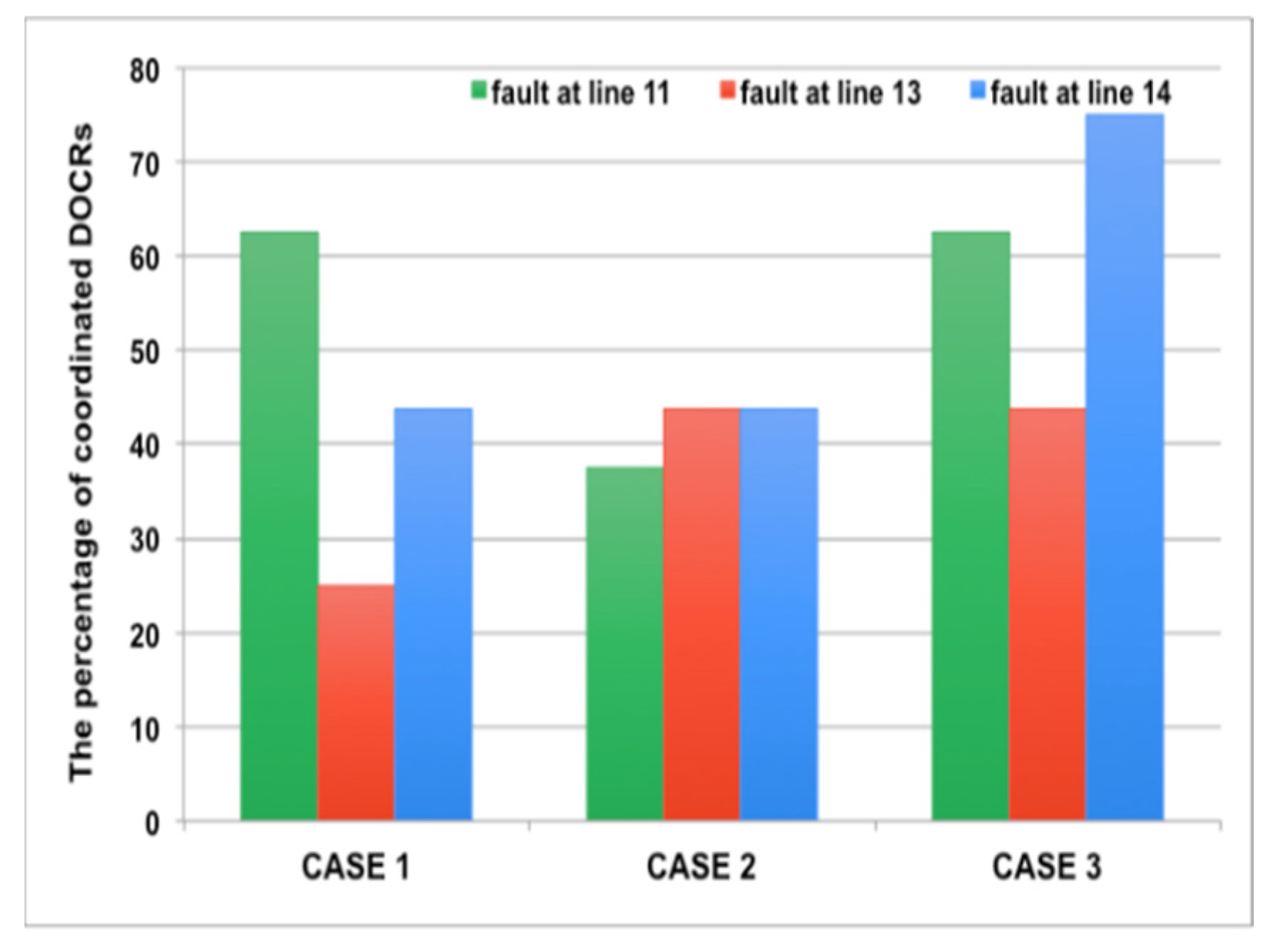
Figure A1 compares the scope of the fault mitigation by showing the percentage of relays in the MG that are reset in response of the failure. It is observed that the percentage of coordinated DOCRs in case#1 when fault at line 11 and case #2 when fault at line 13 does not exceed 62.5%. However, in case #3 (2 DGs are ON) when fault at transmission line 14 between the DGs happens, the percentage of the coordinated relays surpasses 70%. We conclude that the size of the containment zone grows with the increased number of active DGs and the location of the fault.
Figure A1.
The percentage of coordinated DOCRs for each case under fault locations at line 11, line 13, and line 14.
Figure A1.
The percentage of coordinated DOCRs for each case under fault locations at line 11, line 13, and line 14.

Appendix B.2. Comparison on the Effect of DGs and Fault Locations for Baseline IEEE 14 Bus System
To evaluate the responsiveness of our proposed scheme, we performed a test considering the cases (case #1, #2, and #3) and fault locations on (line 11, 13, and 14), while applying the approach of [23]. The objective function of such a baseline approach is commonly used as in the literature and strives to minimize the total operating time of all primary relays in the grid. We compared the total operating time as shown in Table A6. Our proposed protection system enables faster relay coordination, where the total operating time has reduced up to 45% as shown in Figure A2. Thus, our proposed protection system achieves fault containment through the engagement of lower number of relays and faster coordination.
Table A6.
A comparison between the total operating time of the proposed objective function and that of [23].
Table A6.
A comparison between the total operating time of the proposed objective function and that of [23].
| Cases | Fault Location | The Total Operating Time in Second | |
|---|---|---|---|
| Proposed Objective Function | The Objective Function of [23] | ||
| Case #1 | Line 11 | 7.2206 | 9.764 |
| Line 13 | 4.9528 | 8.8631 | |
| Line 14 | 8.0486 | 12.977 | |
| Case #2 | Line 11 | 5.1861 | 7.864 |
| Line 13 | 10.7304 | 15.3445 | |
| Line 14 | 12.0135 | 19.986 | |
| Case #3 | Line 11 | 7.6653 | 9.9786 |
| Line 13 | 8.2684 | 12.975 | |
| Line 14 | 12.6324 | 18.9753 | |
Figure A2.
Percentage of reduction in the total operating time for each case under fault locations at line 11, line 13, and line 14.
Figure A2.
Percentage of reduction in the total operating time for each case under fault locations at line 11, line 13, and line 14.

Appendix B.3. High DG-Penetrated Microgrid Test for IEEE15-Bus System
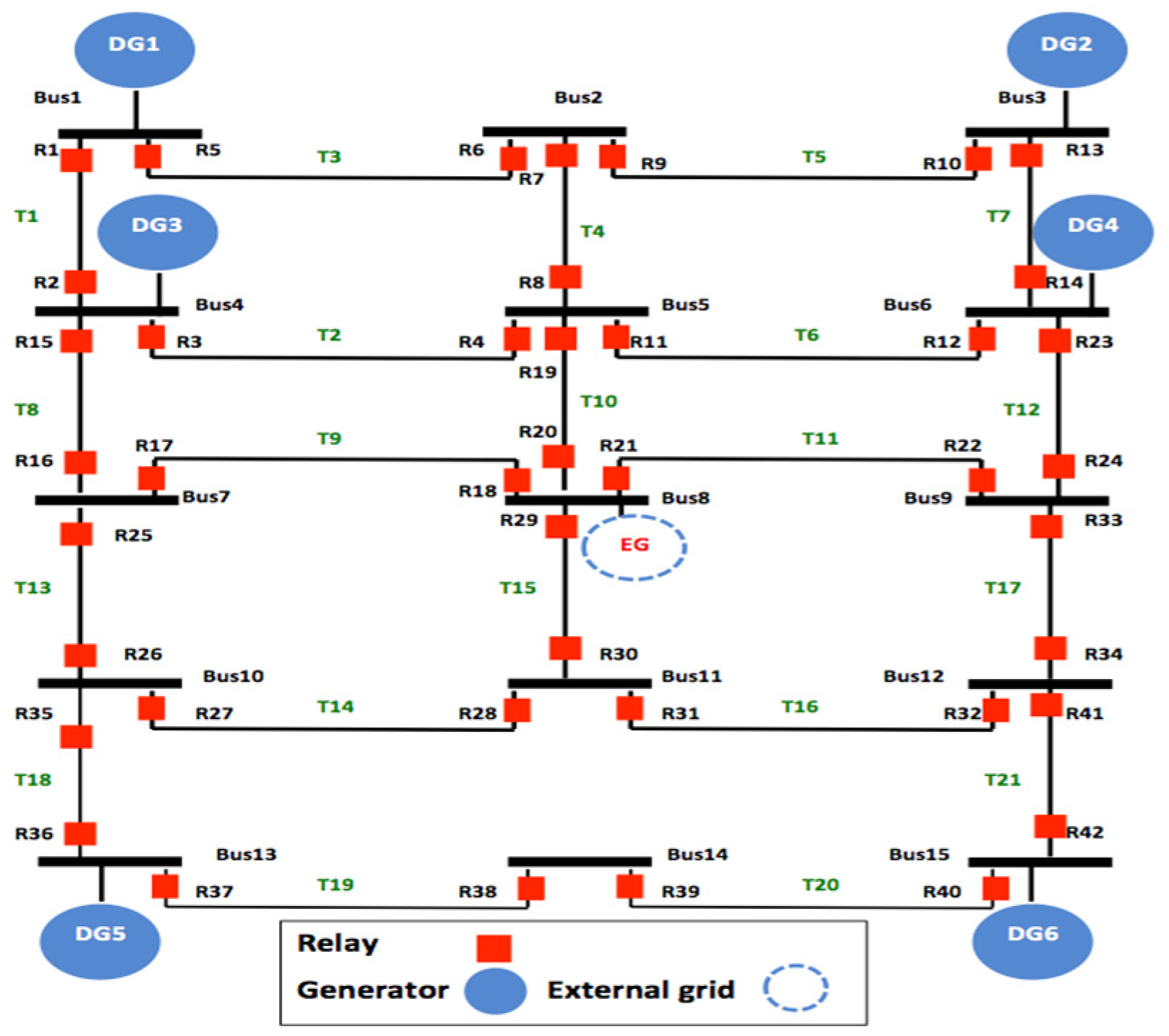
IEEE 15 bus system is an example of highly DG-penetrated distribution networks. We are considering the configuration shown in Figure A3. This configuration incorporates 15 buses, 21 transmission lines, and hence it has 42 directional overcurrent relays. All DGs have ratings of 15 MVA, 20 kV and a synchronous reactance of x = 15%. Similarly, all the transmission lines have impedance of Z = 0.19 + j0.46 Ω/km. bus 8 is connected to an external grid that is modeled by 200 MVA short-circuit capacity [47].
Figure A3.
A single-line diagram showing IEEE 15 Bus system as MG with highly distributed generators.
Figure A3.
A single-line diagram showing IEEE 15 Bus system as MG with highly distributed generators.
IEEE 15-Bus System
We have also applied our approach to the IEEE 15-bus system; such a system is highly penetrated with DGs. We adopt the configuration and the specification of [47]. Several tests have been conducted on different fault locations e.g., 19, 4, 16, 12 transmission lines. For brevity, we have selected the fault located on transmission line 4 (T4) between buses 2, 5 where relays #7 and #8 are placed as depicted in Figure A4; because (T4) is strategically located in the center between four DGs. In this configuration, the CTI is 0.2 and the relays sense the fault simultaneously.
Figure A4.
Capturing the containment zone for a fault at line 4 for IEEE 15 system.
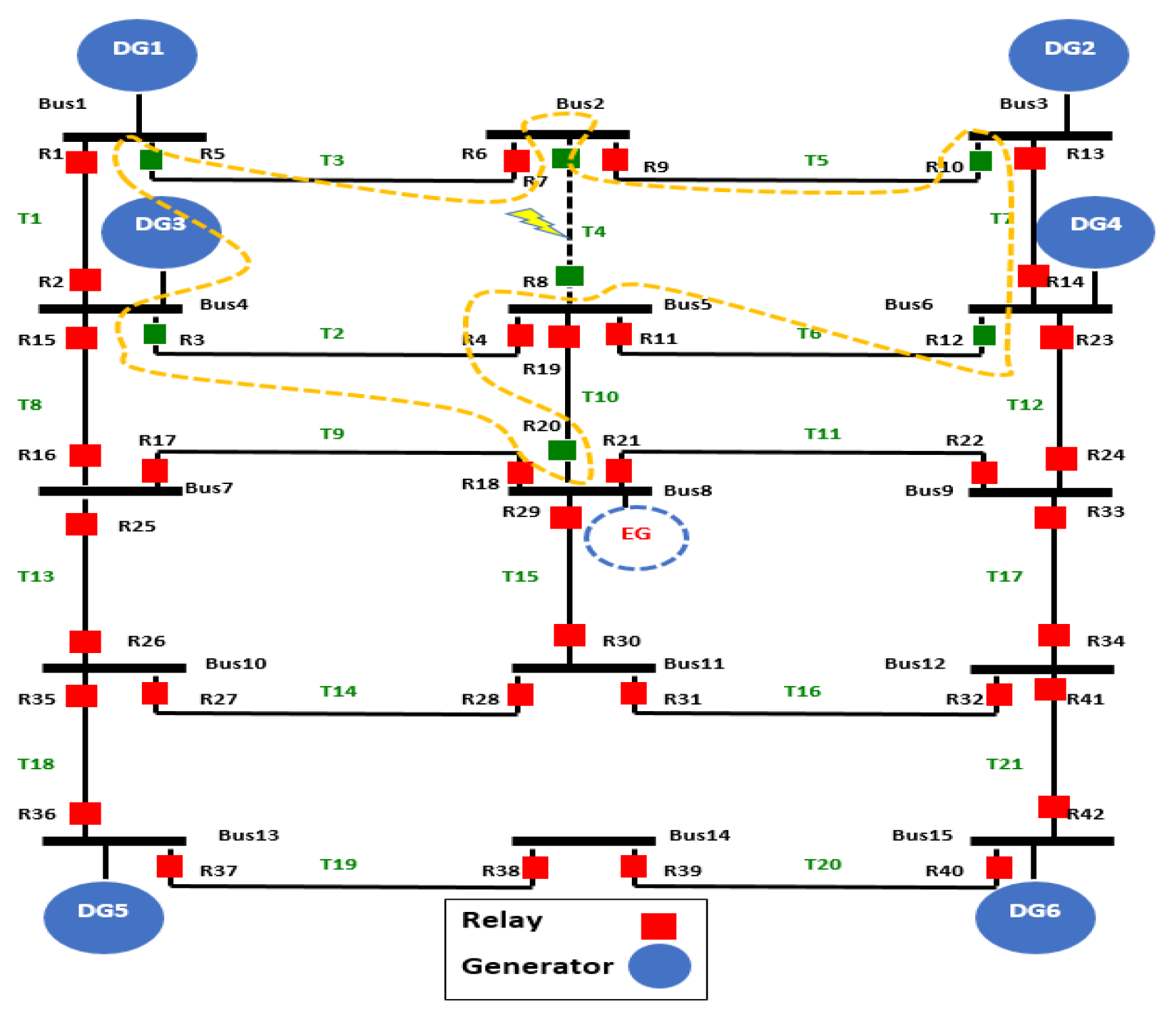
To identify the containment zone, we have measured the operating time of relays #7 and #8 during the fault; the operating time of both relays is found to be 0.302 s. The plug setting (PS) and the time dial setting (TDS) for relay #7 are 1.0238 s, and 0.8921 s, respectively; the corresponding values for relay #8 are 1.260 s, and 0.391 s. We have then calculated the operating time of the backup relays that are connected to buses 2 and 5 from other transmission lines, as seen in Figure A4. The operating time of relays #3, #5, #10, #12 and #20 is 0.102 s, which is over zero. Hence, these relays will be involved within the containment zone.
The operating time of further outward backup relays is −0.098. As mentioned in previous tests, any calculated relay operating time that is less than zero will not be involved in the containment zone. Thus, the boundary of the containment zone is marked, as a yellow dashed line in Figure A4 and the impacted relays considered for coordination are 7 relays where the number of relays affected by the fault is 16.66% of total relays in the MG. Table A7 presents the plug setting, the time dial setting, and the operating time of the coordinated relays within the containment zone. The total operating time of these relays is 3.85 s. The computational execution time of the optimal solution with our proposed algorithm is 0.2993 s.
Table A7.
The DOCR settings and the operating time when fault occurred at transmission line 4 (T4).
| Containment Zone Relays | TDS | PS | Operating Time (s) |
|---|---|---|---|
| Relay 3 | 1.08 | 1.88 | 0.48 |
| Relay 5 | 0.92 | 2.41 | 0.52 |
| Relay 7 | 0.97 | 1.56 | 0.91 |
| Relay 8 | 0.99 | 1.02 | 0.25 |
| Relay10 | 0.43 | 0.54 | 0.81 |
| Relay12 | 0.47 | 2.39 | 0.37 |
| Relay20 | 0.42 | 2.22 | 0.51 |
References
- Parhizi, S.; Lotfi, H.; Khodaei, A.; Bahramirad, S. State of the art in research on microgrids: A review. IEEE Access 2015, 3, 890–925. [Google Scholar] [CrossRef]
- Usama, M.; Moghavvemi, M.; Mokhlis, H.; Mansor, N.N.; Farooq, H.; Pourdaryaei, A. Optimal Protection Coordination Scheme for Radial Distribution Network Considering ON/OFF-Grid. IEEE Access 2021, 9, 34921–34937. [Google Scholar] [CrossRef]
- Kumar, G.V.N.; Kumar, B.S.; Rao, B.V.; Sobhan, P.V.S.; Naidu, K.A. Linear programming technique based optimal relay coordination in a radial distribution system. Int. J. Eng. Technol. 2018, 7, 51–55. [Google Scholar] [CrossRef] [Green Version]
- Tsimtsios, A.M.; Safigianni, A.S.; Nikolaidis, V.C. Generalized distance-based protection design for DG integrated MV radial distribution networks—Part II: Application to an actual distribution line. Electr. Power Syst. Res. 2019, 176. [Google Scholar] [CrossRef]
- Alam, M.N. Adaptive Protection Coordination Scheme Using Numerical Directional Overcurrent Relays. IEEE Trans. Ind. Inform. 2019, 15, 64–73. [Google Scholar] [CrossRef]
- Hussain, N.; Nasir, M.; Vasquez, J.C.; Guerrero, J.M. Recent Developments and Challenges on AC Microgrids Fault Detection and Protection Systems—A Review. Energies 2020, 13, 2149. [Google Scholar] [CrossRef]
- Tailor, J.K.; Osman, A. Restoration of fuse-recloser coordination in distribution system with high DG penetration. In Proceedings of the 2008 IEEE Power and Energy Society General Meeting-Conversion and Delivery of Electrical Energy in the 21st Century, Pittsburgh, PA, USA, 20–24 July 2008. [Google Scholar] [CrossRef]
- North American Electric Reliability Corporation. Performance of Distributed Energy Resources During and After System Disturbance Voltage and Frequency Ride-Through Requirements. 2013. Available online: https://www.nerc.com/pa/RAPA/ra/Reliability Assessments DL/IVGTF17_PC_FinalDraft_December_clean.pdf (accessed on 24 November 2020).
- Tsimtsios, A.M.; Korres, G.N.; Nikolaidis, V.C. A pilot-based distance protection scheme for meshed distribution systems with distributed generation. Int. J. Electr. Power Energy Syst. 2018, 105, 454–469. [Google Scholar] [CrossRef]
- Lin, H.; Liu, C.; Guerrero, J.; Vasquez, J.C. Distance protection for microgrids in distribution system. In IECON 2015—41st Annual Conference of the IEEE Industrial Electronics Society; IEEE: Piscataway, NJ, USA, 2015; pp. 731–736. [Google Scholar] [CrossRef] [Green Version]
- Rao, H.V.G.; Prabhu, N.; Mala, R.C. Adaptive Distance Protection for Transmission Lines Incorporating SSSC with Energy Storage Device. IEEE Access 2020, 8, 156017–156026. [Google Scholar] [CrossRef]
- Biller, M.; Jaeger, J.; Mladenovic, I.; Schacherer, C.; Wolter, D.; Stoetzel, M. Protection systems in distribution grids with variable short-circuit conditions. In Proceedings of the 13th International Conference on Development in Power System Protection, Edinburgh, UK, 7–10 March 2016; Volume 2016. [Google Scholar] [CrossRef]
- Ustun, T.S.; Ozansoy, C.; Zayegh, A. Differential protection of microgrids with central protection unit support. In IEEE 2013 Tencon—Spring, TENCONSpring 2013—Conference Proceedings; IEEE: Piscataway, NJ, USA, 2013; pp. 15–19. [Google Scholar] [CrossRef]
- Conti, S.; Raffa, L.; Vagliasindi, U. Innovative solutions for protection schemes in autonomous MV micro-grids. In Proceedings of the 2009 International Conference on Clean Electrical Power, ICCEP 2009, Capri, Italy, 9–11 June 2009; pp. 647–654. [Google Scholar] [CrossRef]
- He, J.; Wang, Z.; Zhang, Q.; Liu, L.; Zhang, D.; Crossley, P.A. Distributed protection for smart substations based on multiple overlapping units. CSEE J. Power Energy Syst. 2016, 2, 44–50. [Google Scholar] [CrossRef]
- Habib, H.F.; Youssef, T.; Cintuglu, M.H.; Mohammed, O.A. Multi-Agent-Based Technique for Fault Location, Isolation, and Service Restoration. IEEE Trans. Ind. Appl. 2017, 53, 1841–1851. [Google Scholar] [CrossRef]
- Choudhary, N.K.; Mohanty, S.R.; Singh, R.K. Protection coordination of over current relays in distribution system with DG and superconducting fault current limiter. In Proceedings of the 2014 Eighteenth National Power Systems Conference, Guwahati, India, 18–20 December 2014. [Google Scholar] [CrossRef]
- Jones, D.; Kumm, J.J. Future distribution feeder protection using directional overcurrent elements. IEEE Trans. Ind. Appl. 2014, 50, 1385–1390. [Google Scholar] [CrossRef]
- Yazdaninejadi, A.; Golshannavaz, S.; Nazarpour, D.; Teimourzadeh, S.; Aminifar, F. Dual-Setting Directional Overcurrent Relays for Protecting Automated Distribution Networks. IEEE Trans. Ind. Inform. 2018, 15, 730–740. [Google Scholar] [CrossRef]
- Darabi, A.; Bagheri, M.; Gharehpetian, G. Dual feasible direction-finding nonlinear programming combined with metaheuristic approaches for exact overcurrent relay coordination. Int. J. Electr. Power Energy Syst. 2019, 114, 105420. [Google Scholar] [CrossRef]
- Alam, M.N. Overcurrent protection of AC microgrids using mixed characteristic curves of relays. Comput. Electr. Eng. 2019, 74, 74–88. [Google Scholar] [CrossRef]
- Ustun, T.S.; Ozansoy, C.; Zayegh, A. Modeling and simulation of a microgrid protection system with central protection unit. In IEEE 2013 Tencon—Spring, TENCONSpring 2013—Conference Proceedings; IEEE: Piscataway, NJ, USA, 2013; pp. 5–9. [Google Scholar] [CrossRef]
- Saleh, K.; Zeineldin, H.H.; El-Saadany, E.F. Optimal Protection Coordination for Microgrids Considering N–1 Contingency. IEEE Trans. Ind. Inform. 2017, 13, 2270–2278. [Google Scholar] [CrossRef]
- Thararak, P.; Jirapong, P. Implementation of Optimal Protection Coordination for Microgrids with Distributed Generations Using Quaternary Protection Scheme. J. Electr. Comput. Eng. 2020. [CrossRef]
- De Souza, A.C.Z.; Santos, M.; Castilla, M.; Miret, J.; de Vicuña, L.G.; Marujo, D. Voltage security in AC microgrids: A power flow-based approach considering droopcontrolled inverters. IET Renew. Power Gener. 2015, 9, 954–960. [Google Scholar] [CrossRef] [Green Version]
- Albatsh, F.M.; Ahmad, S.; Mekhilef, S.; Mokhlis, H.; Hassan, M.A. Optimal Placement of Unified Power Flow Controllers to Improve Dynamic Voltage Stability Using Power System Variable Based Voltage Stability Indices. PLoS ONE 2015, 10, e0123802. [Google Scholar] [CrossRef]
- Guerrero, J.; Vasquez, J.C.; Matas, J.; de Vicuña, L.G.; Castilla, M. Hierarchical control of droop-controlled AC and DC microgrids—A general approach toward standardization. IEEE Trans. Ind. Electron. 2010, 58, 158–172. [Google Scholar] [CrossRef]
- Gopalakrishnan, A.; Kezunovic, M.; McKenna, S.; Hamai, D. Fault location using the distributed parameter transmission line model. IEEE Trans. Power Deliv. 2000, 15, 1169–1174. [Google Scholar] [CrossRef] [Green Version]
- García, L.F.R.; Londoño, S.M.P.; Flórez, J.J.M. Dynamic load modeling for small disturbances using measurement-based parameter estimation method. In Proceedings of the International Symposium on the Quality of Electrical Power, SICEL, Medellín, Colombia, 27–29 November 2013. [Google Scholar]
- Ustun, T.S.; Ozansoy, C.; Zayegh, A. A microgrid protection system with central protection unit and extensive communication. In Proceedings of the 2011 10th International Conference on Environment and Electrical Engineering, Rome, Italy, 8–11 May 2011. [Google Scholar] [CrossRef]
- Monitoring of Power System Quality eBook by Dr. Hidaia Alassouli—1230002137902|Rakuten Kobo United States. Available online: https://www.kobo.com/us/en/ebook/monitoring-of-power-system-quality (accessed on 24 November 2020).
- Andrés, H.R.F.; Hernandez, J.; Trujillo, E.R. Optimal Power Flow in Electrical Microgrids. Energy Power Eng. 2014, 6, 449–458. [Google Scholar] [CrossRef] [Green Version]
- Wei, C.; Fadlullah, Z.M.; Kato, N.; Stojmenovic, I. A novel distributed algorithm for power loss minimizing in Smart Grid. In Proceedings of the 2014 IEEE International Conference on Smart Grid Communications, SmartGridComm 2014, Venice, Italy, 3–6 November 2014; pp. 290–295. [Google Scholar] [CrossRef]
- Sanseverino, E.R.; Di Silvestre, M.L.; Badalamenti, R.; Nguyen, N.Q.; Guerrero, J.M.; Meng, L.; Quang, N.N. Optimal power flow in islanded microgrids using a simple distributed algorithm. Energies 2015, 8, 11493–11514. [Google Scholar] [CrossRef] [Green Version]
- Bernatik, A. Risk Analysis and Management—Trends, Challenges and Emerging Issues; CRC Press: Boca Raton, FL, USA, 2017. [Google Scholar]
- IEEE Xplore Book Abstract—Microgrid Planning and Design: A Concise Guide. Available online: https://ieeexplore.ieee.org/book/8671408 (accessed on 24 November 2020).
- Bevrani, H.; Francois, B.; Ise, T. Microgrid Dynamics and Control; John Wiley & Sons: Hoboken, NJ, USA, 2017. [Google Scholar]
- Srikanth, P.; Rajendra, O.; Yesuraj, A.; Tilak, M.; Raja, K. Load Flow Analysis of IEEE 14 Bus System Using MATLAB. Int. J. Eng. Res. Technol. 2013, 2, 149–155. [Google Scholar]
- Kim, M.-S.; Haider, R.; Cho, G.-J.; Kim, C.-H.; Won, C.-Y.; Chai, J.-S. Comprehensive Review of Islanding Detection Methods for Distributed Generation Systems. Energies 2019, 12, 837. [Google Scholar] [CrossRef] [Green Version]
- Reigosa, D.; Briz, F.; Blanco, C.; García, P.; Guerrero, J.M. Active islanding detection using high frequency signal injection. IEEE Trans. Ind. Appl. 2012, 48, 1588–1597. [Google Scholar] [CrossRef]
- Das, D.; Gurrala, G.; Shenoy, U.J. Transition between grid-connected mode and islanded mode in VSI-fed microgrids. Sādhanā 2017, 42, 1239–1250. [Google Scholar] [CrossRef]
- Cintuglu, M.H.; Ma, T.; Mohammed, O.A. Protection of Autonomous Microgrids Using Agent-Based Distributed Communication. IEEE Trans. Power Deliv. 2016, 32, 351–360. [Google Scholar] [CrossRef]
- Protection of Electricity Distribution Networks, 2nd Edition (Power and Energy): Juan Gers: 9780863413575: Amazon.com: Books. Available online: https://www.amazon.com/Protection-Electricity-Distribution-Networks-Energy/dp/0863413579 (accessed on 24 November 2020).
- Ahshan, R. Modeling and Analysis of a Micro-Grid System Powered by Renewable Energy Sources. Open Renew. Energy J. 2013, 6, 7–22. [Google Scholar] [CrossRef]
- Volume I, Issue II. Estimation of Line Parameters of an IEEE 14 Bus System. 2014. Available online: www.rsisinternational.org (accessed on 24 November 2020).
- Bedekar, P.P.; Bhide, S.R. Optimum coordination of directional overcurrent relays using the hybrid GA-NLP approach. IEEE Trans. Power Deliv. 2011, 26, 109–119. [Google Scholar] [CrossRef]
- Amraee, T. Coordination of directional overcurrent relays using seeker algorithm. IEEE Trans. Power Deliv. 2012, 27, 1415–1422. [Google Scholar] [CrossRef]
Figure 1.
A single-line diagram showing a sample MG that is a part of the IEEE 14 Bus system with distributed generators on buses 6 and 8.
Figure 1.
A single-line diagram showing a sample MG that is a part of the IEEE 14 Bus system with distributed generators on buses 6 and 8.
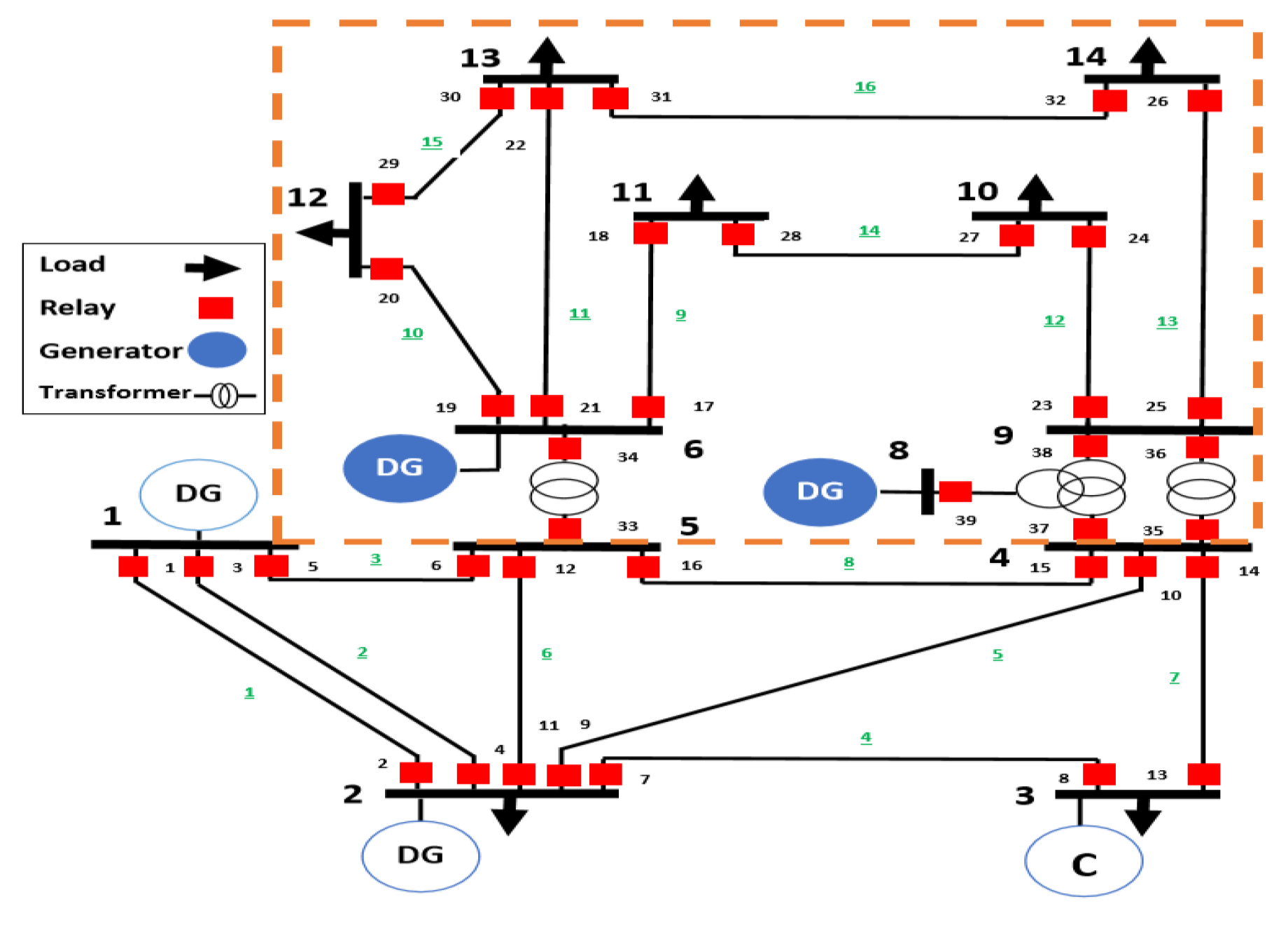
Figure 2.
Communication architecture for a microgrid protection system.

Figure 3.
Flowchart description of the proposed Protection System.
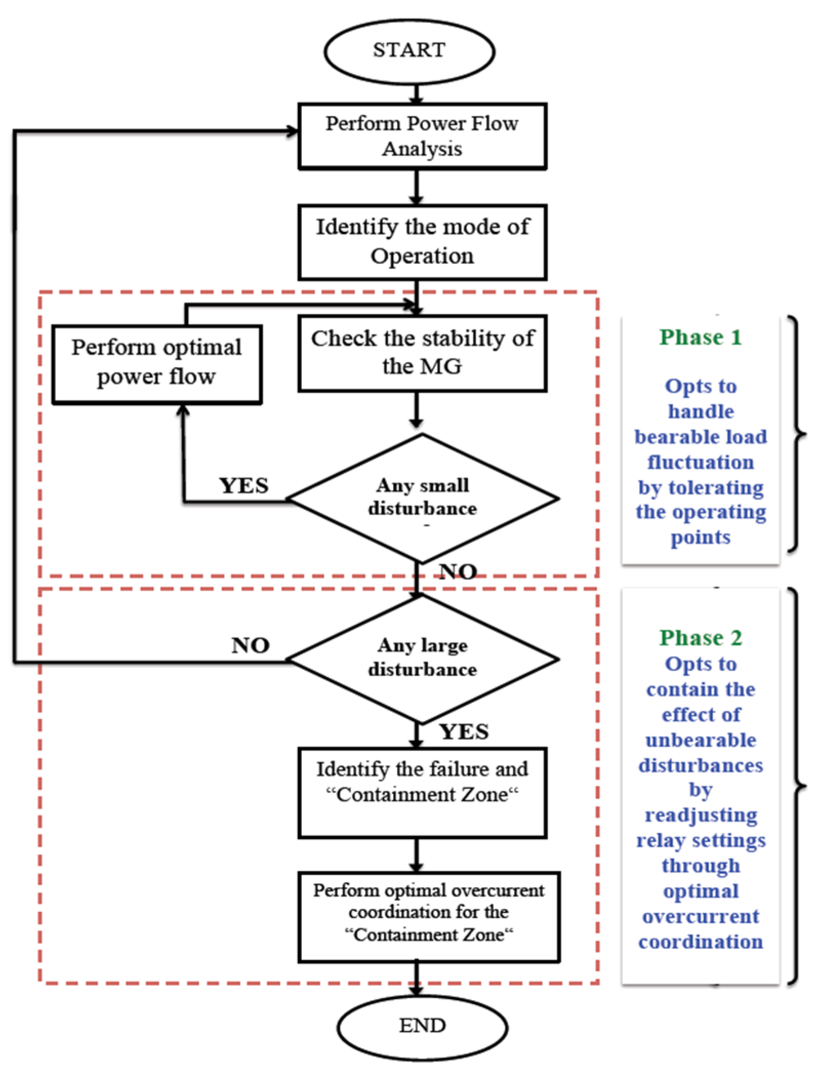
Figure 4.
Illustration of new strategy of identifying the boundaries of the containment zone on a single line diagram of 8 transmission lines and 16 relays.
Figure 4.
Illustration of new strategy of identifying the boundaries of the containment zone on a single line diagram of 8 transmission lines and 16 relays.
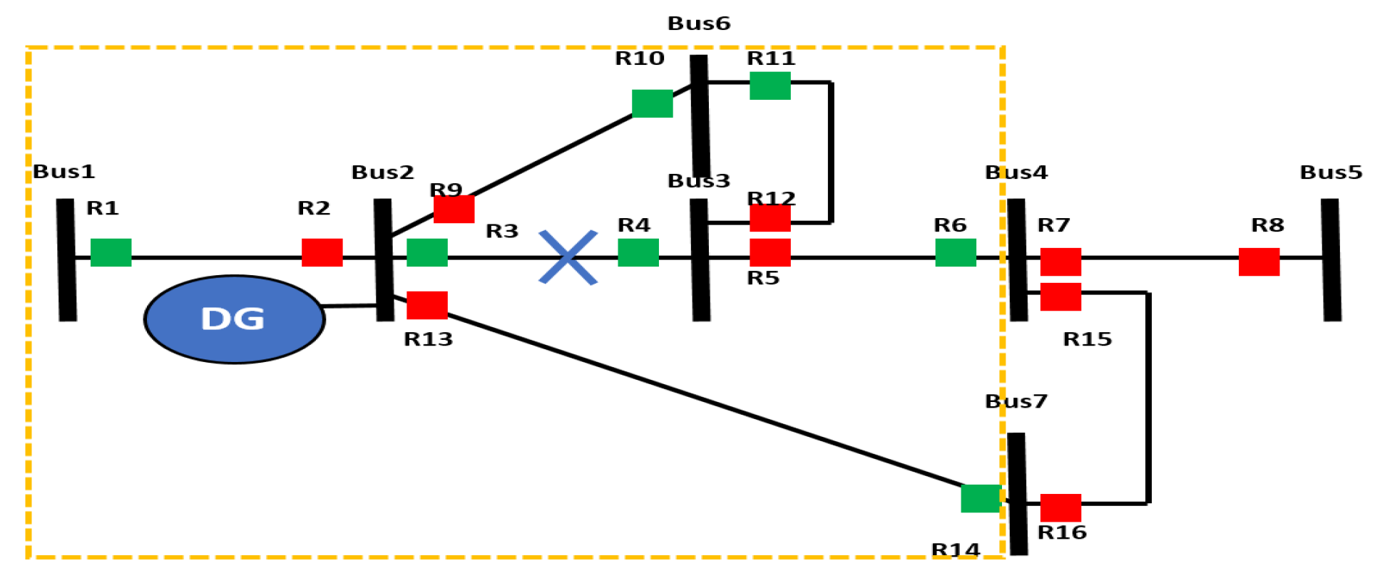
Figure 5.
A single-line diagram showing IEEE 9 Bus system as MG with distributed generator on bus 1.
Figure 5.
A single-line diagram showing IEEE 9 Bus system as MG with distributed generator on bus 1.

Figure 6.
A comparison of the voltage stability in steady state and dynamic load conditions, and the results of applying optimal power flow when load varies for (A) IEEE 9 and (B) IEEE 14.
Figure 6.
A comparison of the voltage stability in steady state and dynamic load conditions, and the results of applying optimal power flow when load varies for (A) IEEE 9 and (B) IEEE 14.

Figure 7.
Capturing the Fault location on transmission line 1 (A), and the relays (Green-colored relays) within containment zone (B) of IEEE 9 bus system.
Figure 7.
Capturing the Fault location on transmission line 1 (A), and the relays (Green-colored relays) within containment zone (B) of IEEE 9 bus system.
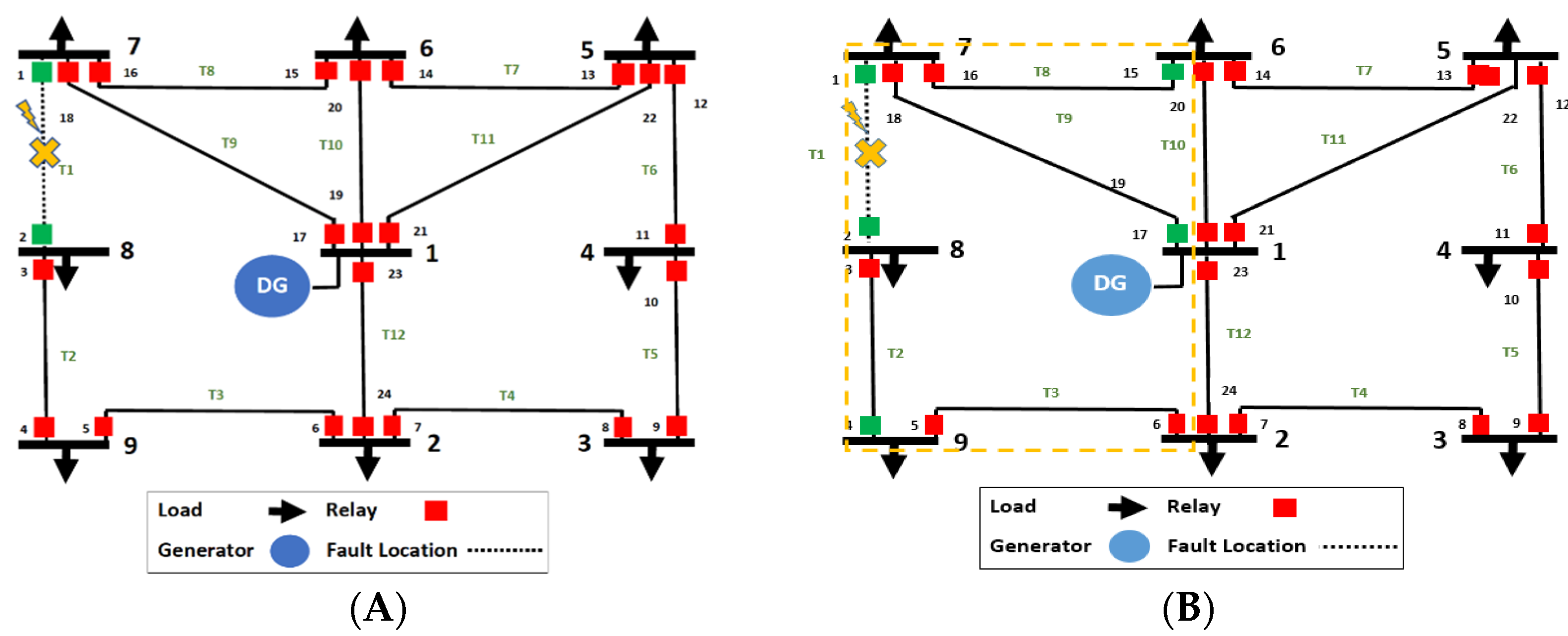
Figure 8.
Capturing the fault location on transmission line 9, and the relays within containment zone of IEEE 14-bus system.
Figure 8.
Capturing the fault location on transmission line 9, and the relays within containment zone of IEEE 14-bus system.
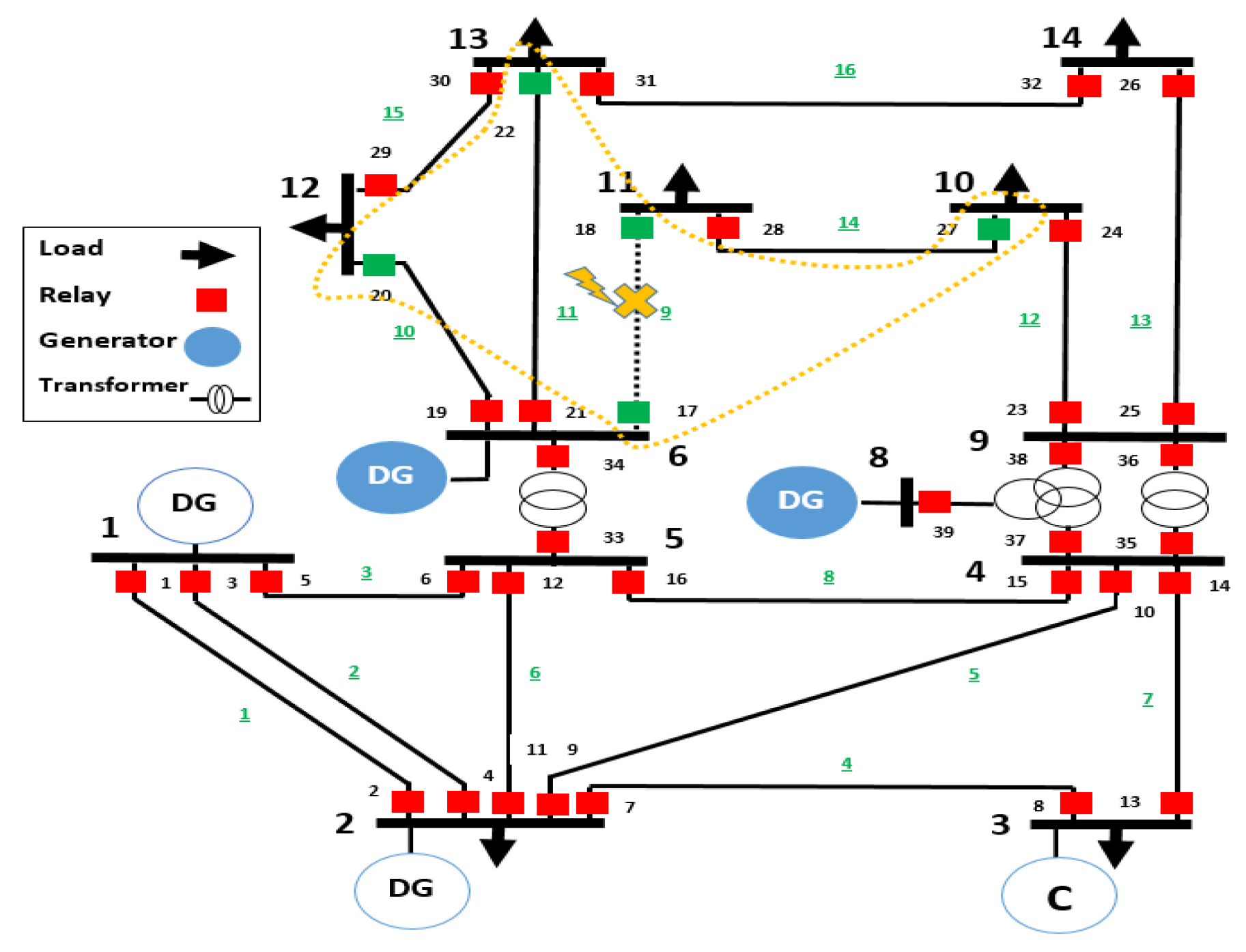
Figure 9.
Capturing the containment zone for one fault at line 16 (A), and for two faults at line 12 and 16 (B) of IEEE 14 bus system.
Figure 9.
Capturing the containment zone for one fault at line 16 (A), and for two faults at line 12 and 16 (B) of IEEE 14 bus system.
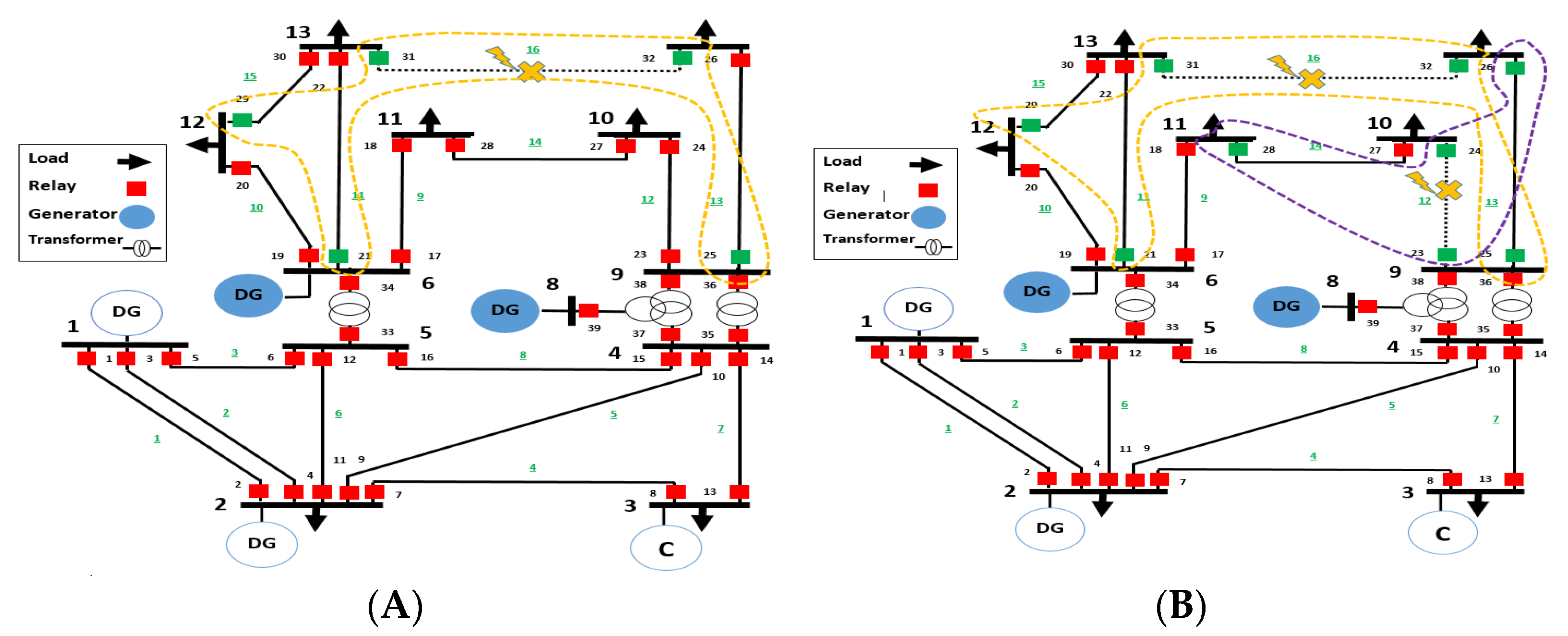
Figure 10.
Capturing the performance of the approach of [23] while handling tolerable disturbance on the IEEE 9 system.
Figure 10.
Capturing the performance of the approach of [23] while handling tolerable disturbance on the IEEE 9 system.
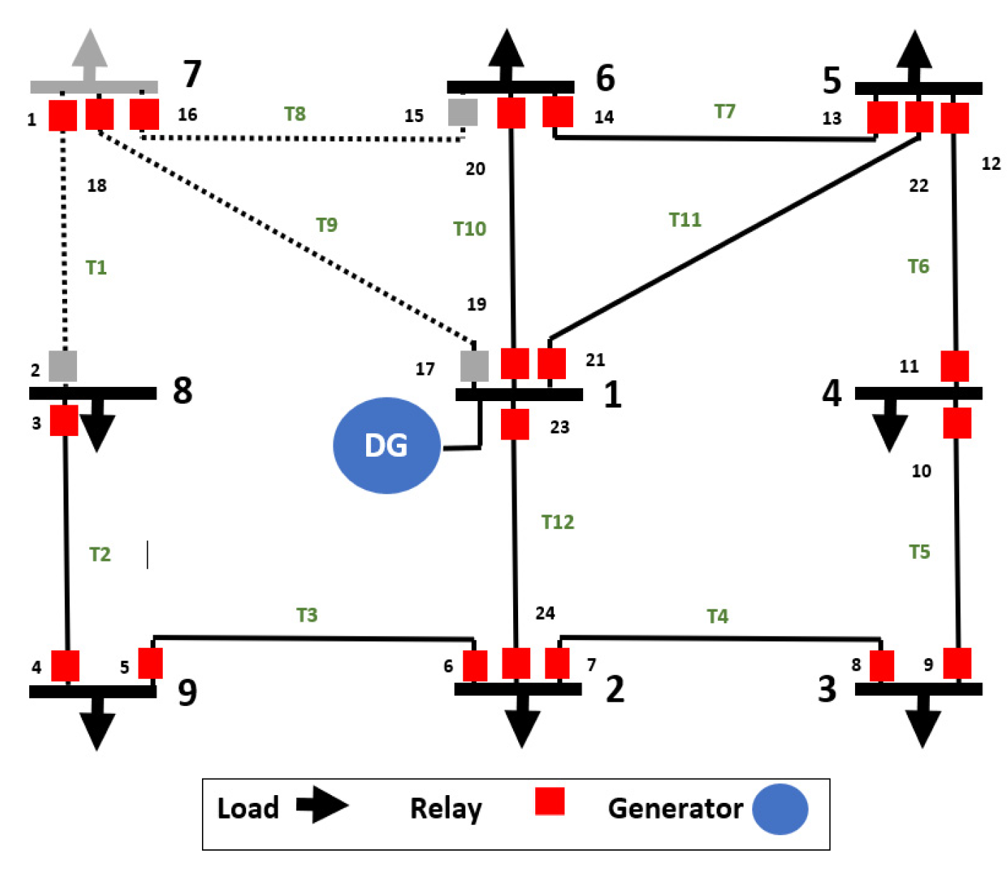
Figure 11.
Capturing the protection performance of the baseline [23] approach on tolerable disturbance for IEEE 14 system.
Figure 11.
Capturing the protection performance of the baseline [23] approach on tolerable disturbance for IEEE 14 system.
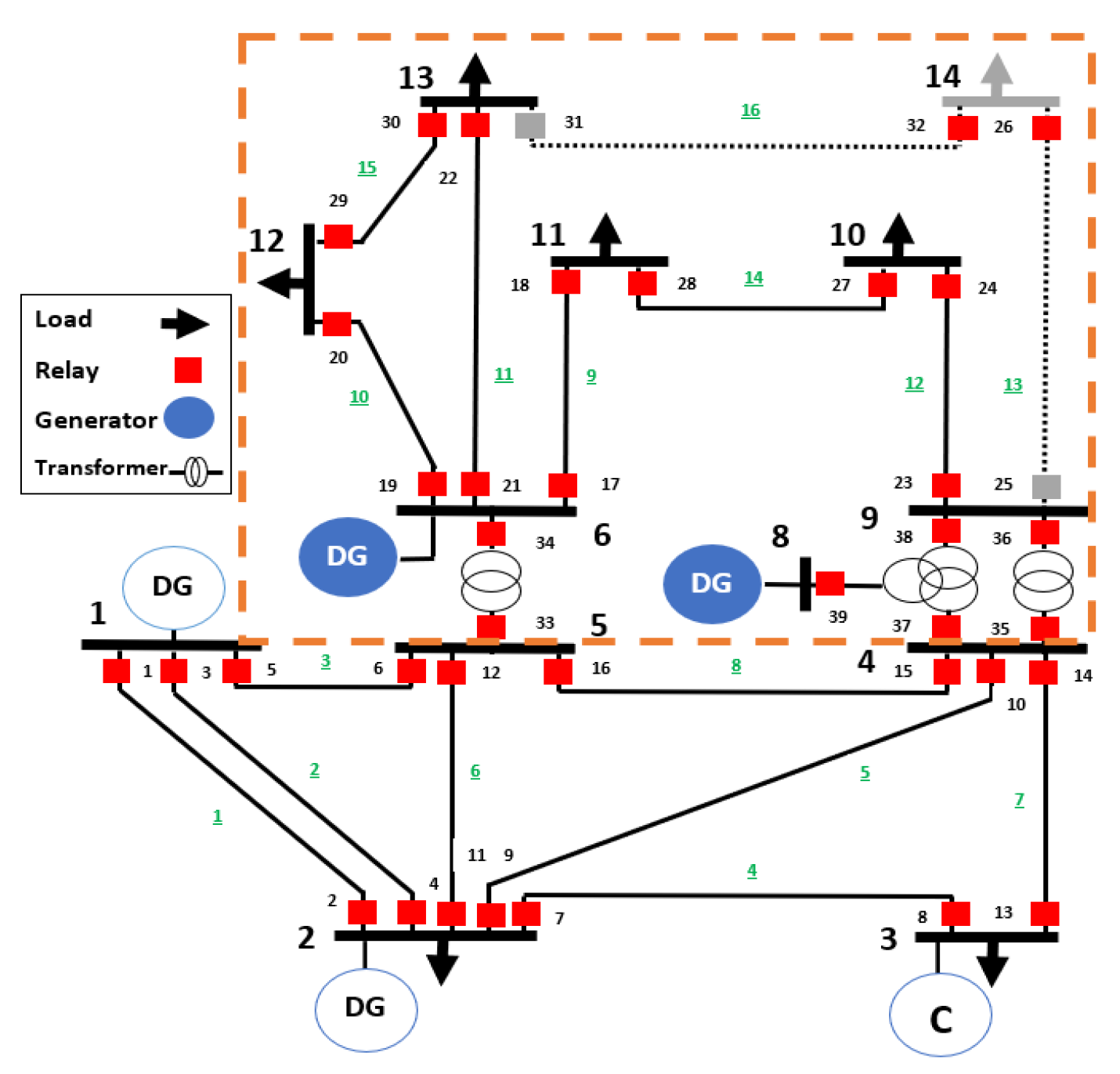
Figure 12.
A single-line diagram showing IEEE 14 Bus system as in with [23] distributed generators on buses 4, 5 and 6.
Figure 12.
A single-line diagram showing IEEE 14 Bus system as in with [23] distributed generators on buses 4, 5 and 6.

Figure 13.
A comparing the total operating time of primary and backup relays of our proposed scheme to that achieved by the approach of [23].
Figure 13.
A comparing the total operating time of primary and backup relays of our proposed scheme to that achieved by the approach of [23].
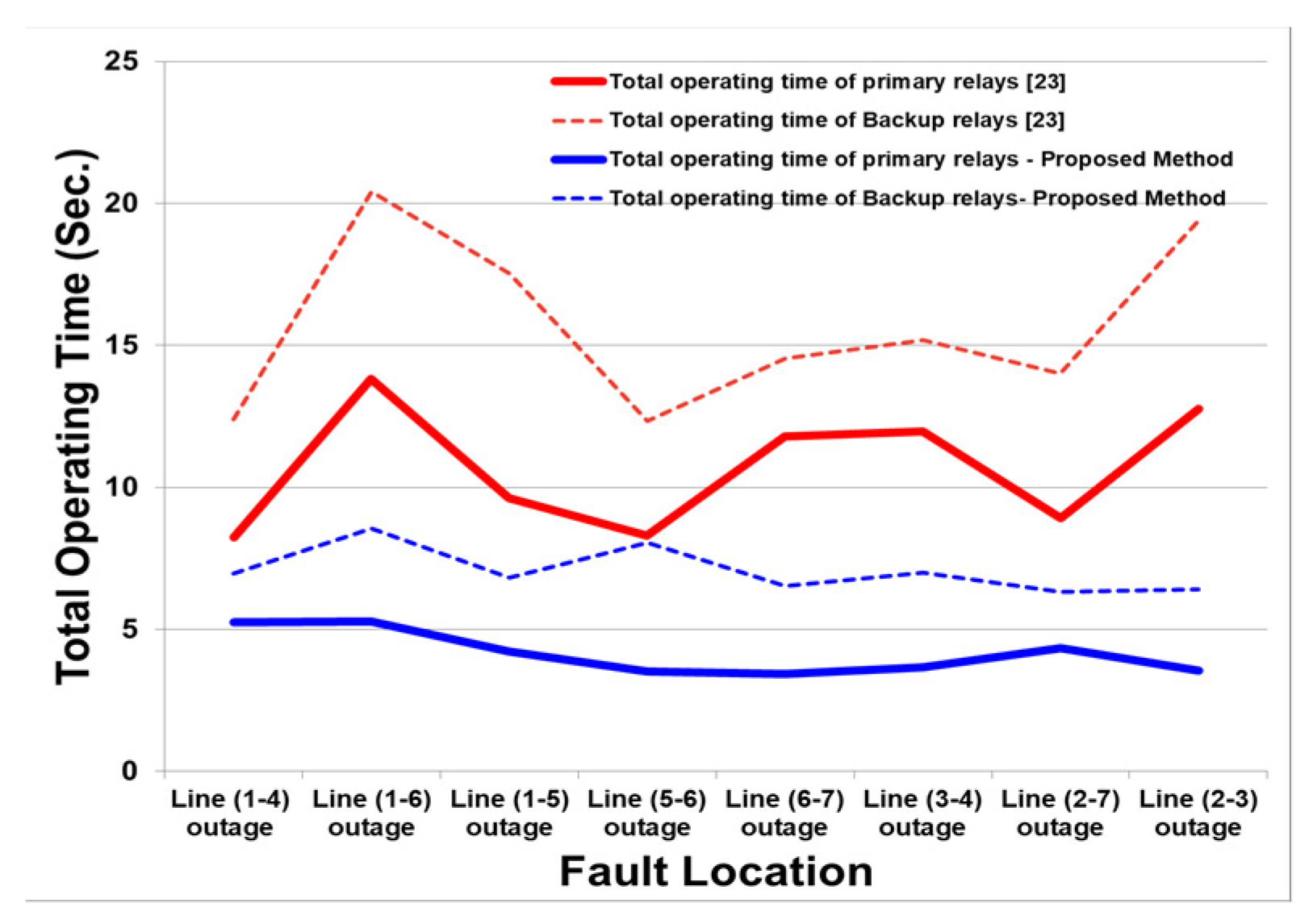
Table 1.
Different protection strategies to address fault current changes.
| Protection Strategy | Advantages | Disadvantages |
|---|---|---|
|
|
|
|
|
|
| ||
|
|
|
|
|
|
|
|
|
|
|
|
Table 2.
MG mode of operation through the status of DGs.
| Mode of Operation | Connected | Islanded |
|---|---|---|
| Active and reactive power (P-Q) | Constant | Variable |
| Voltage and frequency (V-F) | Variable | Constant |
Table 3.
The electrical components specifications.
| Generator’s Specification | Protection Component’s Specification | Protection Component’s Specification | |||
|---|---|---|---|---|---|
| The active power | 102.554 MW | Overcurrent relays type | Schweitzer 351, curve type IEC. | Transmission line current | 1750 Amps |
| The reactive power | 5.597 MVAR | Overcurrent relays pickup range | IDMT, 0.02-3.2 s, 1 Amp | The Apparent power rating | 100 MVA |
| The apparent power | 104.5 VA | Circuit breakers type | Standard SYM | Resistance | R = 0.0001 P.U. |
| The power factor | 95% | Circuit breakers duration | 5-cycle duration, contact parting time (CPT) of 3, and time constant of 45 s. | Reactance | X = 10 P.U. |
| Poles | 4 | Circuit breakers maximum rating | 1.01 KV | Admittance | Y = 0 P.U. |
| Speed | 1500 RPM | Transformer ratio | 500:1 | ||
| Full-Load Amperes (FLA) rating | 1925 | ||||
| Impedance | Xd” = 10%; Xd”/Ra = 19; Ra = 0.052105 Ohms | ||||
Table 4.
The location and capability for the DG units associated with the Considered Microgrid based IEEE 14.
Table 4.
The location and capability for the DG units associated with the Considered Microgrid based IEEE 14.
| DG No. | DG Location | Capacity of Synchronous Generators (MVA) |
|---|---|---|
| DG unit 1 | 6 | 100 |
| DG unit 2 | 8 | 100 |
Table 5.
The characteristics of Overcurrent relays IEC standard.
| Curve Description | Standard | α | β | L |
|---|---|---|---|---|
| Standard inverse | IEC | 0.02 | 0.14 | 0 |
Table 6.
The DOCR settings and the operating time after the optimization process when fault occurred at transmission line 1 (T1).
Table 6.
The DOCR settings and the operating time after the optimization process when fault occurred at transmission line 1 (T1).
| Containment Zone Relays | TDS | PS | Operating Time (s) |
|---|---|---|---|
| Relay 1 | 0.026210 | 0.021952 | 0.0257 |
| Relay 2 | 0.028915 | 0.025359 | 0.0237 |
| Relay 4 | 0.028039 | 0.024171 | 0.0359 |
| Relay 15 | 0.026001 | 0.026902 | 0.2253 |
| Relay 17 | 0.528113 | 0.559173 | 0.0341 |
Table 7.
The affected relays corresponding to each fault location.
| Fault Location | Containment Zone Relays | Operate. Time (s) |
|---|---|---|
| Tran. Line (T1) | Relay (1, 2, 4, 15, 17) | 0.3447 |
| Tran. Line (T2) | Relay (2, 3, 1, 6) | 0.1029 |
| Tran. Line (T3) | Relay (4, 5, 3, 8, 23) | 0.4311 |
| Tran. Line (T4) | Relay (7, 8, 10, 23) | 0.4236 |
| Tran. Line (T5) | Relay (7, 9, 10, 22) | 0.1409 |
| Tran. Line (T6) | Relay (11, 22, 9, 14, 21) | 0.3265 |
| Tran. Line (T7) | Relay (13, 14, 11, 16, 19, 21) | 0.3461 |
| Tran. Line (T8) | Relay (15, 16, 17, 2, 19, 13) | 0.4522 |
| Tran. Line (T9) | Relay (17, 18, 2, 15) | 0.539 |
| Tran. Line (T10) | Relay (19, 20, 13, 16) | 0.4875 |
| Tran. Line (T11) | Relay (21, 22, 11, 14) | 0.5018 |
| Tran. Line (T12) | Relay (23, 24, 5, 8) | 0.3049 |
Table 8.
The DOCR settings and the operating time when fault occurred at transmission line 9 (T9).
| Containment Zone Relays | TDS | PS | Operating Time (s) |
|---|---|---|---|
| Relay 17 | 0.3218 | 1.6721 | 1.3860 |
| Relay 18 | 0.1783 | 1.1743 | 1.3582 |
| Relay 20 | 0.2852 | 2.4265 | 1.3026 |
| Relay 22 | 0.4190 | 1.9308 | 1.2995 |
| Relay 27 | 0.4013 | 2.2003 | 1.3381 |
Table 9.
The involved relays (within the containment zone) and its total operating time when the scope of the failure grows.
Table 9.
The involved relays (within the containment zone) and its total operating time when the scope of the failure grows.
| Fault Location | Containment Zone Relays | Total Operating Time (s) |
|---|---|---|
| Tran. Line (T16) | Relay (21, 25, 29, 31, 32) | 7.9531 |
| Tran. Line (T16, T12) | Relay (21, 23, 24, 25, 26, 28 29, 31, 32) | 8.8793 |
| Tran. Line (T12, T15, T16) | Relay (19, 21, 23, 24, 25, 26, 28 29, 30, 31, 32) | 9.6779 |
| Tran. Line (T12, T14, T15, T16) | Relay (17, 19, 21, 23, 24, 25, 26, 27, 28, 29, 30, 31, 32) | 10.6148 |
Table 10.
The list of impacted relays and their settings when tolerable disturbance is experienced in the IEEE 9, 14 configurations.
Table 10.
The list of impacted relays and their settings when tolerable disturbance is experienced in the IEEE 9, 14 configurations.
| Config. | Relay No. | TDS | PS | Max. Current in Normal Operation (Amps.) | Current during Dynamic Loads(Amps.) |
|---|---|---|---|---|---|
| IEEE 9 Bus System | 2 | 0.0383 | 0.0231 | 108.33 | 124.09 |
| 15 | 0.0261 | 0.0260 | 96.34 | 110.53 | |
| 17 | 0.0295 | 0.0322 | 388.91 | 403.81 | |
| IEEE 14 Bus System | 25 | 0.3962 | 2.7504 | 194.10 | 224.07 |
| 31 | 0.3885 | 2.9884 | 369.92 | 381.03 |
Table 11.
A comparison of total operating time between the proposed protection scheme and that of [23] for different fault location.
Table 11.
A comparison of total operating time between the proposed protection scheme and that of [23] for different fault location.
| Fault Location | Total Operating Time in (s) | ||
|---|---|---|---|
| [23] | Proposed Scheme | Reduction | |
| Line (1–4) outage | 20.6281 | 13.2155 | 35.93% |
| Line (1–6) outage | 27.1609 | 14.9852 | 44.82% |
| Line (1–5) outage | 34.2278 | 14.0431 | 58.97% |
| Line (5–6) outage | 22.9395 | 10.2297 | 55.40% |
| Line (6–7) outage | 32.1598 | 9.9875 | 68.94% |
| Line (3–4) outage | 27.1606 | 10.9409 | 59.71% |
| Line (2–7) outage | 26.3331 | 9.8911 | 62.44% |
| Line (2–3) outage | 20.6281 | 12.1005 | 41.34% |
Table 12.
The DOCR settings and the operating time for baseline [23] when fault occurred at transmission line 1 (T1).
Table 12.
The DOCR settings and the operating time for baseline [23] when fault occurred at transmission line 1 (T1).
| Relay No. | TDS | PS | Operating Time (s) |
|---|---|---|---|
| 1 | 0.021525 | 0.021621 | 0.0163801 |
| 2 | 0.026352 | 0.021475 | 0.0298431 |
| 3 | 0.033039 | 0.020311 | 0.0296611 |
| 4 | 0.023705 | 0.026102 | 0.0280651 |
| 5 | 0.027107 | 0.024631 | 0.0296401 |
| 6 | 0.025357 | 0.023533 | 0.0227431 |
| 7 | 0.025357 | 0.020961 | 0.0251802 |
| 8 | 0.027012 | 0.029731 | 0.0269221 |
| 9 | 0.026041 | 0.020173 | 0.0260221 |
| 10 | 0.033461 | 0.021762 | 0.0290762 |
| 11 | 0.021752 | 0.023075 | 0.0320891 |
| 12 | 0.027093 | 0.023387 | 0.0821091 |
| 13 | 0.027201 | 0.023387 | 0.0392731 |
| 14 | 0.025441 | 0.023853 | 0.0392731 |
| 15 | 0.021359 | 0.175344 | 0.0286422 |
| 16 | 0.025991 | 0.543573 | 0.0273281 |
| 17 | 0.020836 | 0.246732 | 0.0205129 |
| 18 | 0.534511 | 0.720311 | 0.0321467 |
| 19 | 0.833215 | 0.032125 | 0.0276543 |
| 20 | 1.199532 | 0.025321 | 0.0290762 |
| 21 | 1.197021 | 0.246323 | 0.0346218 |
| 22 | 0.025012 | 0.021473 | 0.0296401 |
| 23 | 1.245122 | 0.722562 | 0.0290762 |
| 24 | 1.206718 | 1.097653 | 0.0296401 |
Table 13.
A comparison of total operating time between the proposed protection scheme and that of [23] for fault located on transmission line 1.
Table 13.
A comparison of total operating time between the proposed protection scheme and that of [23] for fault located on transmission line 1.
| Proposed Protection System | Baseline [23] | |
|---|---|---|
| Operating Time (s) | 0.3464 | 0.7446 |
Table 14.
The total operating time of our proposed protection system and that of [23] for each fault location.
Table 14.
The total operating time of our proposed protection system and that of [23] for each fault location.
| Fault Location | Operate. Time (s) | % of Total Operating Time Reduction | |
|---|---|---|---|
| Proposed Protection System | Baseline [23] | ||
| Tran. Line (T1) | 0.3464 | 0.7446 | 53.479 |
| Tran. Line (T2) | 0.1006 | 0. 2813 | 64.237 |
| Tran. Line (T3) | 0.4293 | 0.8296 | 48.252 |
| Tran. Line (T4) | 0.4292 | 0.8527 | 48.298 |
| Tran. Line (T5) | 0.1373 | 0.3011 | 54.400 |
| Tran. Line (T6) | 0.3159 | 0.6731 | 53.067 |
| Tran. Line (T7) | 0.2950 | 0.7042 | 58.108 |
| Tran. Line (T8) | 0.4494 | 0.7219 | 37.747 |
| Tran. Line (T9) | 0.5022 | 0.8633 | 41.828 |
| Tran. Line (T10) | 0.4976 | 0.8245 | 39.648 |
| Tran. Line (T11) | 0.5022 | 0.8904 | 43.591 |
| Tran. Line (T12) | 0.3024 | 0.6991 | 56.744 |
Table 15.
The DOCR settings and the operating time for baseline [23] when single fault occurred at transmission line 9.
Table 15.
The DOCR settings and the operating time for baseline [23] when single fault occurred at transmission line 9.
| Relay No. | TDS | PS | Operating Time (s) |
|---|---|---|---|
| 17 | 0.309864 | 1.673021 | 1.102216 |
| 18 | 0.068321 | 1.912391 | 0.108317 |
| 19 | 0.205115 | 1.037233 | 1.262101 |
| 20 | 0.054012 | 1.175339 | 0.523014 |
| 21 | 0.135661 | 1.912391 | 1.328115 |
| 22 | 0.360196 | 1.673021 | 0.122958 |
| 23 | 0.059984 | 1.292341 | 0.942339 |
| 24 | 0.124201 | 2.428312 | 0.048322 |
| 25 | 0.139448 | 1.862502 | 1.028258 |
| 26 | 0.054012 | 1.424142 | 0.202446 |
| 27 | 0.308124 | 2.428312 | 0.754291 |
| 28 | 0.092321 | 1.862502 | 1.754992 |
| 29 | 0.064983 | 1.382232 | 0.983201 |
| 30 | 0.111439 | 0.753319 | 0.212933 |
| 31 | 0.050637 | 1.673021 | 0.521991 |
| 32 | 0.055116 | 1.093202 | 1.319982 |
| 33 | 0.137887 | 1.029344 | 0.643301 |
| 34 | 0.111439 | 2.428312 | 1.411826 |
| 35 | 0.181019 | 1.091193 | 0.237662 |
| 36 | 0.124201 | 1.175339 | 1.902366 |
| 37 | 0.071998 | 1.862502 | 1.123101 |
| 38 | 0.081445 | 1.082322 | 0.927311 |
Table 16.
Comparing the total operating time of the proposed protection scheme and that of [23] for a single fault and multiple independent faults.
Table 16.
Comparing the total operating time of the proposed protection scheme and that of [23] for a single fault and multiple independent faults.
| Total Operating Time (s) | Proposed Protection System | Baseline [23] | % of Coordinated DOCRs |
|---|---|---|---|
| Single fault in line (9) | 6.6844 | 18.4610 | 36.98% |
| Multiple independent faults line (16) | 7.9531 | 19.2988 | 41.10% |
| Multiple independent faults line (12, 16) | 8.8793 | 21.7641 | 40.79% |
| Multiple independent faults line (12, 15, 16) | 9.6779 | 22.5852 | 42.61% |
| Multiple independent faults line (12, 14, 15, 16) | 10.6148 | 23.9832 | 44.37% |
Publisher’s Note: MDPI stays neutral with regard to jurisdictional claims in published maps and institutional affiliations. |
© 2021 by the authors. Licensee MDPI, Basel, Switzerland. This article is an open access article distributed under the terms and conditions of the Creative Commons Attribution (CC BY) license (https://creativecommons.org/licenses/by/4.0/).
Share and Cite
MDPI and ACS Style
Bawayan, H.; Younis, M. Microgrid Protection through Adaptive Overcurrent Relay Coordination. Electricity 2021, 2, 524-553. https://doi.org/10.3390/electricity2040031
AMA Style
Bawayan H, Younis M. Microgrid Protection through Adaptive Overcurrent Relay Coordination. Electricity. 2021; 2(4):524-553. https://doi.org/10.3390/electricity2040031
Chicago/Turabian StyleBawayan, Haneen, and Mohamed Younis. 2021. "Microgrid Protection through Adaptive Overcurrent Relay Coordination" Electricity 2, no. 4: 524-553. https://doi.org/10.3390/electricity2040031