Article

Voltage Unbalance, Power Factor and Losses Optimization in Electrified Railways Using an Electronic Balancer

1
Department of Electrical and Computers Engineering, University of Porto, Rua Roberto Frias, 4200-465 Porto, Portugal
2
SNCF Réseau, Département Traction Électrique, 6 Avenue François Mitterrand, 93574 La Plaine Saint Denis, France
*
Author to whom correspondence should be addressed.
Electricity 2021, 2(4), 554-572; https://doi.org/10.3390/electricity2040032
Submission received: 3 October 2021 / Revised: 8 November 2021 / Accepted: 9 November 2021 / Published: 12 November 2021

Abstract

:
Unbalanced currents, low power factor and high losses contribute to increasing the bill infrastructure managers must pay to the TSO/DSO operator that supplies electric energy to the railway system. Additionally, if regenerative energy coming from braking regimes is not allowed to be injected into the grid or even is penalized when it occurs, then the optimization of those parameters must be pursued. One of the possible measures that can be taken to counteract those phenomena is the installation of electronic balancers in heavy loaded substations in order to optimize the interface to the three-phase electric grid. This paper shows the benefit of such use taking examples from real conditions and realistic simulations assumed equivalent to field measurements.

1. Introduction

In the European Union there is an important increase underway in railway traffic either in terms of passenger trains or in terms of freight trains. The constitution of the Shift2Rail (S2R) Joint Undertaking (JU) is a driving force framed in the Horizon 2020 to tackle the rising issues in this domain [1]. Among several others funded by the S2R JU, the IN2STEMPO project is a large spectrum, one that has many and quite different objectives. One of the most important is the study and demonstration of solutions based on Flexible AC Transmission Systems (FACTS) devices capable of improving the performance of the railway system [2].
The increasing traffic in almost all electrified railway lines also increases the power demand from the transmission/distribution system operator (TSO/DSO). However, an important part of the connected traction power substations (TPSS) present an electrical interface to the high voltage (HV) or extra high voltage (EHV) grid that is far from optimal regarding some relevant parameters. Pure single-phase connections, or based on V/V transformers or on Scott or Leblanc transformers, present to the electric grid an equivalent unbalanced load.
In the past, solutions like the Steinmetz compensation scheme were used to mitigate the unbalance until a certain level. The process of balancing the traction power substation current can be divided into two types: Passive balancing (fixed Steinmetz network) and active balancing (variable current source). The passive Steinmetz compensation circuit can achieve the balanced condition in a specific load power operating point. However, the fixed impedance of a conventional Steinmetz compensation circuit does not provide the variable equivalent impedance required by the highly variable traction loads if the compensation is supposed to be made in the full load range. Still, it must be mentioned that Steinmetz compensation circuits with variable equivalent impedances were researched [3].
The fixed passive impedances are replaced by controllable currents through power semiconductor devices (e.g., thyristors); the system is designated a Static Var Compensator (SVC). However, two relevant issues can occur when using the thyristor-based active Steinmetz system: The converter injects low-frequency harmonic currents into the electric grid even when low-frequency tuned filters are used [4], and, due to an unknown equivalent grid impedance there is the risk of potential resonances created by them [5].
Recently, new power electronics devices and converter topologies allowed the development of advanced versions of the Steinmetz compensation circuit, either as single converters [6,7,8,9] or hybrid solutions [10,11]. Thyristor-based or IGBT-based these compensators are active balancers since they do not behave as variable equivalent impedances in parallel with the point of common coupling but, instead, they act as variable current sources according to the operation point of the railway load.
Only modern architectures, all based on power electronics converters, like the Static Frequency Converter (SFC) [12,13], the co-phase arrangement [14,15], or the Rail Power Conditioner (RPC) [16,17], are capable of interfacing with the grid in an optimized way, i.e., balanced three-phase load, near sinusoidal currents and almost unitary power factor. However, these solutions require a special transformer like the RPC or the co-phase architectures, or dual-stage converters, as is the case of the SFC.
The electronic balancer is a power electronics based system belonging to the FACTS family and performs functions that improve some parameters of the railway electric system. An electronic balancer is a universal solution since it is connected in parallel with the point of common coupling (PCC) of the substation and so does not require a special transformer.
Its main architecture is similar to the active power filter or the Static Synchronous Compensator (STATCOM), and its main function in railway applications is to balance the three-phase currents although it can also compensate the reactive power thus increasing the power factor in the three-phase grid. The balancer also acts as an active filter, having the capability of compensating harmonic currents in a limited low-frequency range [8,18,19]. Relevant and positive side effects of balancer usage are better power quality and increased energy efficiency, very important keywords in today’s electric railways industry [20,21,22].
In recent scientific literature, several works have addressed the problem of voltage/current unbalance. With experimental validation, in [23] the authors propose the usage of a modular multilevel converter STATCOM to solve the effects of an unbalanced load, where the injection of the third harmonic enables a more optimal operation. To cope with train regeneration which causes a necessary increase in the compensator capacity, the authors in [24] propose a hybrid topology with a modular multilevel converter railway power conditioner and a magnetic controlled reactor where the capacity of the devices can be reduced when compared with a traditional architecture.
The impact in the power grid of an increasing number of High Speed Railway (HSR) lines together with the increase of renewable energy sources has also been addressed. The adoption of STATCOM solutions to mitigate these issues has been reviewed in [25]. In [26] is presented a three-stage pre-assessment process taking into consideration the grid connection scheme, towards an evaluation for the need of a compensator in the TPSS. In [27] is studied the integration of wind farms and the HSR power system, when both geographically coexist in weak power grids of remote areas. Specifically, the impact of the intermittent TPSS power consumption will cause performance reduction of Doubly Fed Induction Generator (DFIG) wind turbines. The solution proposed by the authors and further extended by [28] is to propose a variable voltage unbalance factor target reference for the railway STATCOM and the DFIG wind turbines, to cope with the standards and to improve the DFIG wind turbine operation.
The objective of this paper is then the evaluation of the impact in the three-phase grid of installing an electronic balancer in the railway electrical infrastructure. In particular, it is focused on analyzing the resulting current and voltage unbalance factors, the power factor and the power losses. The optimization of these parameters can be mandatory through standards (e.g., the requirements set in [29,30]) and/or contractual agreements or, if optional, they bring benefits in terms of energy costs. Accordingly, only the steady-state condition is of relevance in the work, with the dynamics of the balancer operation not being relevant and, as such, not considered in the presented analysis.

2. Voltage Unbalance Factor, Power Factor and Losses

The architecture considered in this paper is the single-phase connection of a substation to the HV/EHV grid, as shown in Figure 1. The three relevant parameters under analysis are the voltage unbalance factor ( V UF ), the power factor in the three-phase and the grid losses.

2.1. Voltage Unbalance in the Three-Phase Grid

When seen from the three-phase grid, the single-phase substation current is an unbalanced one. Then, the three-phase current can be decomposed into a positive sequence component (PSC), a negative sequence component (NSC), and a zero sequence component (ZSC), which is null when there is no neutral wire [31]. The three sequences of currents (positive: I ̲ 1 , negative: I ̲ 2 and zero: I ̲ 0 ) are obtained from the currents in the tree-phase system ( I ̲ a , I ̲ b , and I ̲ c ) by:
I ̲ 1 I ̲ 2 I ̲ 0 = 1 3 1 a a 2 1 a 2 a 1 1 1 I ̲ a I ̲ b I ̲ c
where a = exp ( j 2 π / 3 ) . It should be mentioned that the decomposition is valid either in transient conditions (time domain) or in steady-state (phasor domain). In this work only the steady-state condition is relevant and the symmetrical components decomposition provides three phasors: I ̲ 1 , I ̲ 2 and I ̲ 0 .
The main consequence of having a negative sequence component in the current is the appearance of a negative sequence component in the three-phase voltage. This is a highly negative factor that is penalized by either power quality standards or TSO/DSO operators. The voltage unbalance factor is defined as the ratio between the magnitude of the negative sequence component ( V ̲ 2 ) and the positive sequence component ( V ̲ 1 ) and is highly limited in quality of service regulations, grid codes and in relevant standards [29]:
V UF ( % ) = | V ̲ 2 | | V ̲ 1 | · 100
Considering the assumption that the negative sequence impedance is equal to the positive sequence one (either in high-voltage or in medium-voltage levels), the V UF factor is also equal to the ratio between the NSC and the PSC components of the three-phase current. An accurate estimate of the produced voltage unbalance factor was demonstrated in [32] and is given by:
V UF S L S L + S SC 3 ϕ
where S L is the actual apparent power of the single-phase load and S SC 3 ϕ is the three-phase short-circuit apparent power of the grid at the point of connection of the load, i.e. the primary side of the TPSS traction substation in this study.
Nevertheless, it should be noted that, if no additional compensation measures are taken, the voltage unbalance factor tends to be higher when the TPSS is connected to HV grids than when connected to EHV grids. This is due to the lower short-circuit equivalent impedance of HV grids compared to EHV grids. Then, the connection to EHV grids could be a solution to avoid excessive V UF values but, usually, it is more expensive than the connection to HV ones [33]. Thus, compensating the NSC of the three-phase current using electronic balancers is of major importance for infrastructure managers leading to the existence of an important market of technological solutions, supplied by major industrial companies, to solve this issue.

2.2. Three-Phase Power Factor

The power factor in a three-phase system with the presence of negative and zero sequence components of currents, as a result of unbalanced three-phase loads, has different interpretations regarding the definition of apparent power [34]. In this work we use the definition of power factor for the unbalanced load which includes the definition of apparent power suggested by Buchholz known as Fryze Buchholz Depenbrock (FBD) theory [35]. According to this theory, in three-phase, three-wire systems, the three-phase active power (named collective active power, P Σ ) is defined as:
P Σ = 1 T 0 T ( v a * i a + v b * i b + v c * i c ) d t
where v k * is the instantaneous voltage measured between phase k and a virtual star point common to all phases and i k is the phase k current. Similarly, the apparent power (named collective apparent power, S Σ ) is defined as:
S Σ = V a * 2 + V b * 2 + V c * 2 · I a 2 + I b 2 + I c 2
where V k * and I k are the root mean square (r.m.s.) values of the voltage and current in phase k, respectively. Using the two above defined powers, the collective power factor is defined by:
P F Σ = P Σ S Σ
and expresses an important power quality aspect of the three-phase power circuit.
An alternative to the FBD theory for estimating the power factor in the three-phase grid could be the one recommended in IEEE standard 1459 [36]. However, it can be concluded that, for the conditions assumed in this work, namely a balanced voltage system without harmonic distortion, the two definitions produce the same result.

2.3. Power Losses

Another important electric grid parameter is the three-phase power losses. Not only the global efficiency of the system is affected but also high losses cause excessive heat in the conductors and rise their temperature, reducing the reliability. For the calculation of this parameter, the equivalent impedance of the electric grid represented in Figure 1 (Thévenin equivalent) is considered and obtained from TSO/DSO information. Parameters R g and j ω L g are the equivalent positive sequence impedance of the grid. As example, in an unbalanced condition the equivalent traction current flows only through phases a and b, being zero in phase c. If the equivalent traction current (defined by I ̲ Tr ) has a r.m.s. value of I Tr then the power losses in the unbalanced three-phase system, P LossU are given by:
P LossU = 2 R g I ̲ Tr 2
In the three-phase system the resulting current are given by:
I ̲ a = I ̲ Tr e j π / 6 I ̲ b = I ̲ Tr e j 5 π / 6 I ̲ c = 0
Assuming that the equivalent traction current has a power factor expressed by P F = cos ϕ then, using (1), it can be obtained the three sequences of the three-phase current. In this case, the positive, negative and zero sequences are given, respectively, by:
I ̲ 1 = 1 / 3 · I ̲ Tr e j ϕ I ̲ 2 = 1 / 3 · I ̲ Tr e j ( ϕ π / 3 ) I ̲ 0 = 0
When the balancer compensates the negative sequence of the load current the three-phase current becomes balanced and the losses ( P LossB ) are now only originated by I ̲ 1 and are given by:
P LossB = R g I ̲ Tr 2
It can be concluded that a substantial loss reduction of 50% is achieved if a balanced current circulates in the three-phase grid for the same load power.
If the operation mode of the electronic balancer is set to compensate also the power factor then a further reduction of the losses can be obtained ( P LossPF ) through the reduction of the r.m.s. value of the current. In this case they are given by:
P LossPF = R g I ̲ Tr 2 ( P F ) 2
This last losses factor reduction depends only on the power factor value (and not on the absolute power value). Eventually, this reduction is not too important in order to justify the other effects it has in the sizing (e.g., semiconductors, dc-bus capacitor) and structure of the converter [37].

3. Electronic Balancer
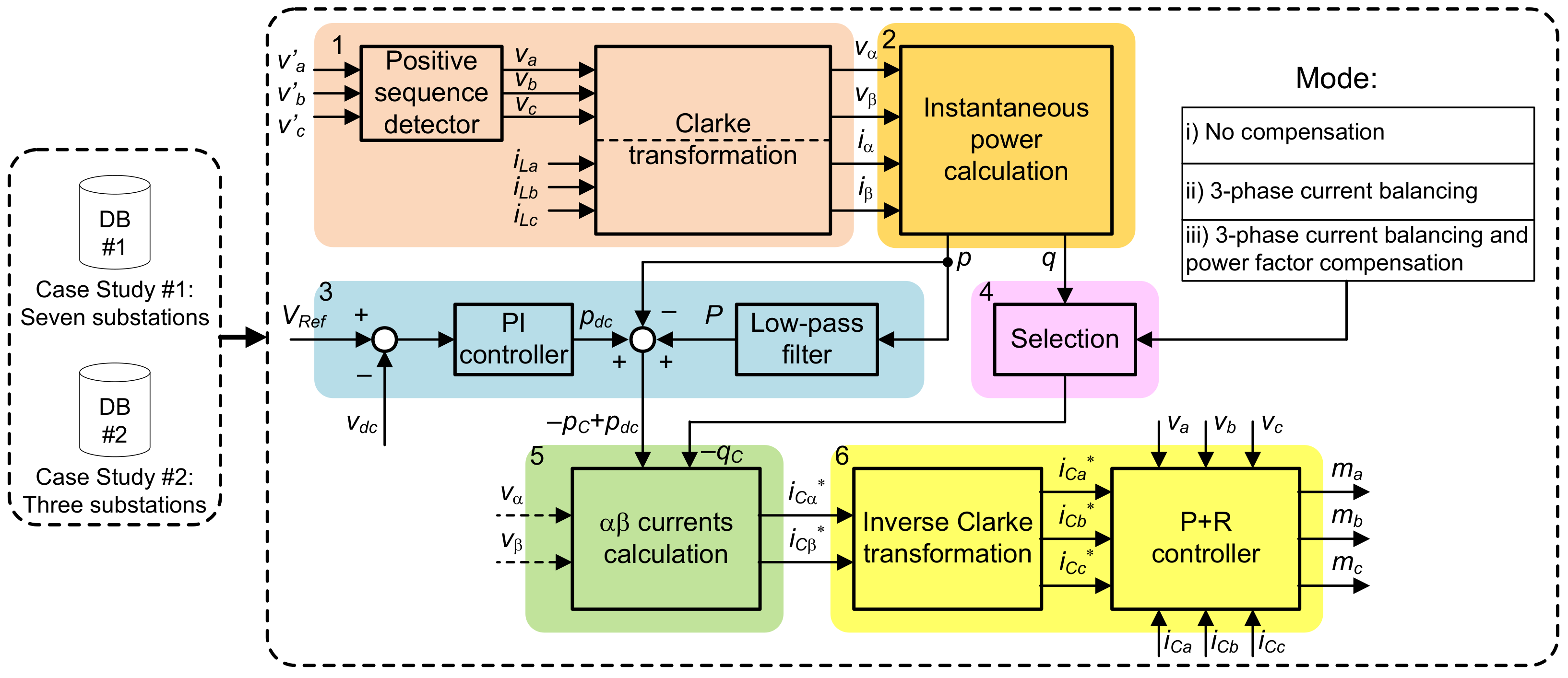
The functionality of an electronic balancer can be reached with a three-phase dc/ac power electronic converter without active power flow capability at the dc-bus. It can manage reactive power and, in doing so, it can also redirect active power between its phases, independently of the TPSS architecture: Single-phase, V-V (as shown in Figure 2a), or other. The converter power structure can vary to a great extent but, in the medium to high power range, the modular multilevel structure in its different arrangements (in Figure 2b) is exemplified the full-bridge one) tends to have more advantages than its alternatives [19,37]. In terms of three-phase grid interface the converter behaves like a conventional one and its upper layer control structure is well known.
Among several alternatives to implement the control functions, the main ones used in this work are based on [38,39] and can be organized as: (1) Positive sequence extraction of the fundamental grid voltage, V ̲ 1 , through a phase-locked loop (PLL) followed by a Clarke transformation of the three-phase voltages and currents; (2) instantaneous real and imaginary power calculation, p ( t ) and q ( t ) , respectively, in ( α , β ) axes; (3) estimation of the average active power flow and dc-bus losses compensation; (4) mode selection between: (i) No compensation, (ii) three-phase current balancing only or (iii) three-phase current balancing and power factor compensation; (5) definition of the compensation current in ( α , β ) axes; (6) inverse Clarke transformation and closed loop control of the three-phase currents (using proportional-resonant controllers). It should be mentioned that the control algorithm also compensates low-frequency current harmonics [18]. The main block diagram of the Balancer controller implementing the above functions is shown in Figure 3, according to the following brief description.
In an electric system intended to be balanced and containing only a positive sequence of voltages, the presence of negative sequence components can be a major problem. In this condition, it is shown that the active power supplied by the network is given by [40]:
P = 3 V 1 I 1 cos ( ϕ 1 ) + 3 V 2 I 2 cos ( ϕ 2 )
where V 1 , V 2 , I 1 and I 2 are the root-mean-square values of the positive and negative sequence components of the voltage and current in the electric grid, respectively, and ϕ 1 ( ϕ 2 ) is the phase displacement between the voltage and current of the positive (negative) sequence. Thus, the positive and negative sequence components of voltage and current contribute to the active power. It is therefore necessary to develop and apply a control method that properly addresses this condition, as in [38]. Since the fundamental objective of the compensation system is to impose balanced currents on the grid then, under this condition, the active power will be associated only with the positive sequence component of the grid voltage (estimated with block 1 in Figure 3). In this work an a b c axes scalar control method is proposed for the AC currents, but methods such as α β axes control or d q (vector) axes control, among others, could also be used [41]. The pq-theory was selected as the power control method [40]. In a three-phase, three-wire system, the a b c α β Clarke transformation of voltages and currents, also included in block 1 of Figure 3, is given by:
v α v β = 2 3 1 1 / 2 1 / 2 0 3 / 2 3 / 2 v a v b v c
The instantaneous powers, real and imaginary, p and q, respectively, are given by (see block 2 in Figure 3):
p q = v α v β v β v α i α i β
For the selection of the compensation mode for the imaginary power q c is the instantaneous imaginary power to be compensated (block 4 in Figure 3). For this application two options are possible: Current balancing only or current balancing and power factor correction. In both cases, harmonics compensation is included but in a limited range, according to the above mentioned restrictions. In any condition, the dc-bus power losses, p dc , must be supplied by the electric grid (block 3 in Figure 3). Then, the compensation currents references in α β axes (output of block 5 in Figure 3) are given by:
i C α * i C β * = 1 v α 2 + v β 2 v α v β v β v α p C + p d c q C
The inverse Clarke transformation, α β a b c , which provides the three-phase AC currents references (block 6 in Figure 3) for the converter is given by:
i C a * i C b * i C c * = 1 0 1 / 2 3 / 2 1 / 2 3 / 2 i C α * i C β *
The Proportional plus Resonant controller (PR) has been elected for the control of the AC currents with zero steady-state error. The Laplace transform of the ideal PR controller is:
G P R ( s ) = K P r + 2 K I r s s 2 + ω 0 2
where K P r and K I r are design parameters and ω 0 is the grid angular frequency. Since this work is mainly concerned with three-phase current balancing, losses and power factor, it is assumed that there are no harmonics either in the three-phase voltages or the load currents. Accordingly, there is no need of additional controllers, tuned for rejecting the load current low-frequency harmonics.
It should be noted that the current control could be implemented in α β axes, with two PR controllers instead of three [40,42]. However, in the three-phase version it is more simple to include the current limits in each phase because when compensating the power factor, the three-phase currents at the converter output become themselves unbalanced.
Thus, in steady-state, the Balancer operation eliminates the NSC component of the current in the three-phase grid and, if defined by the mode of operation, also compensates all the remaining three-phase reactive power. In this way, the power factor in the three-phase grid can be increased to near unitary and the power losses can be reduced if the current magnitude is also reduced.
As stated in the Introduction, only the steady-state operation is relevant in this work. It is assumed that the Balancer operation does not affect the grid voltage and thus the load current is considered an independent variable. The analysis presented in this work depends on a dataset of measurements (in fact, realistic simulations) in each substations, where this data is an output of the Horizon 2020 IN2STEMPO project. The methodology is based on evaluation framework based on Matlab, where this framework uses the dataset to generate results regarding the voltage unbalance factor, the power factor and power losses in the three-phase grid. These results, presented in this paper in the following sections, refer to different conditions according to the Balancer mode of operation; that being:
(i)
No compensation: There is no compensation of the unbalanced three-phase current; the system operates as is.
(ii)
Load current balancing: Only the negative sequence of the three-phase current is compensated by the Balancer.
(iii)
Load current balancing and power factor correction: The negative sequence ( I ̲ 2 ) of the three-phase current is compensated for load balancing, and unitary power factor is reached by compensating the imaginary/reactive part of the positive sequence of the three-phase current.
The algorithm processes output data from domain-specific software (quasi-instantaneous apparent power consumption with a time step of 1 s) obtained for two case studies: The first one related to a near 250 km railway line which includes seven traction power substations and a second case study with a near 290 km line comprising three substations.

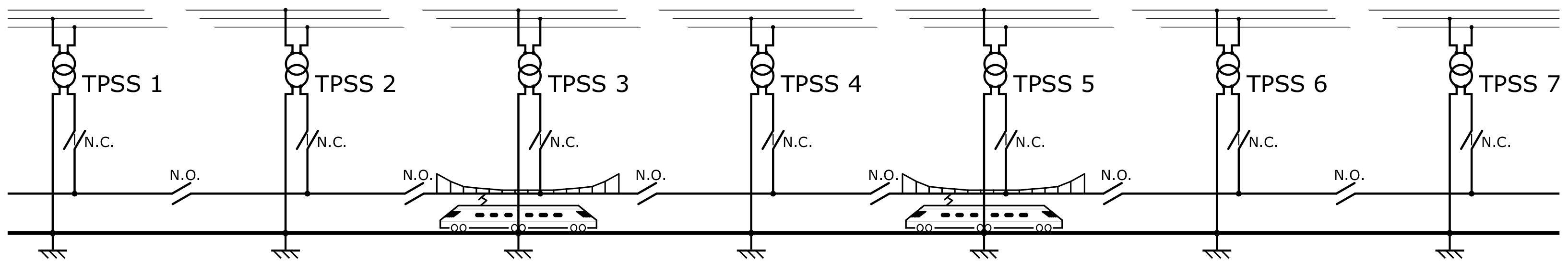
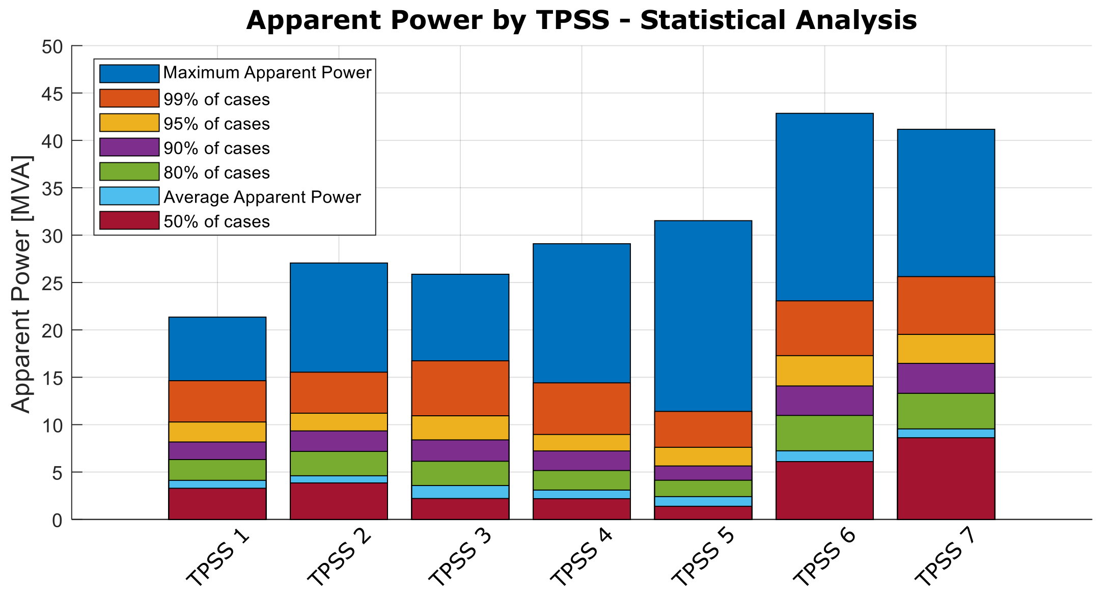
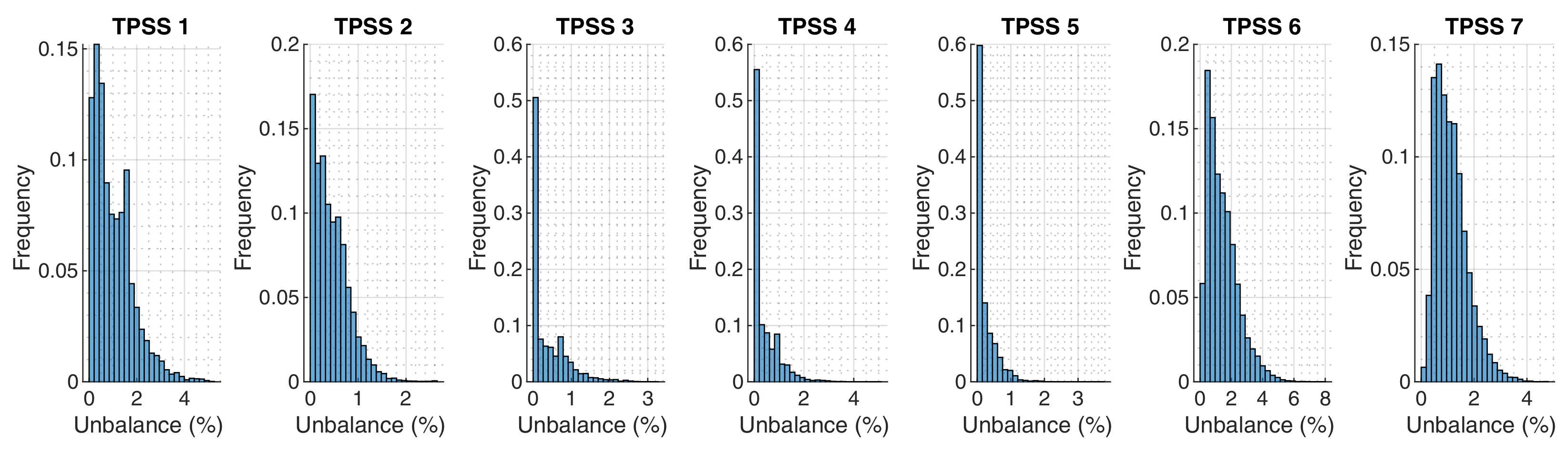
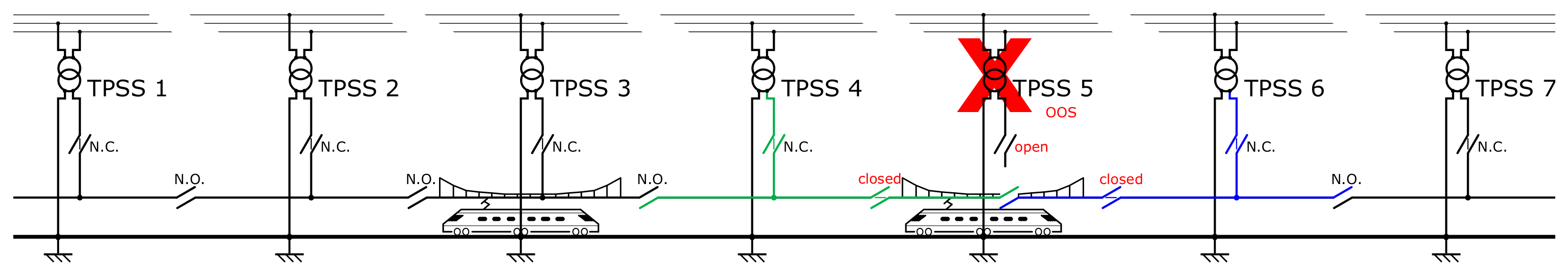
4. Case Study #1: Seven Substations

Case study #1 is a line constituted by seven substations according to the diagram in Figure 4.
For this line, and using the results from the simulated operation, Figure 5 shows the range of apparent power as a percentage of the samples (samples of 1 s) that appears during the period between 05:00 o’clock and 24:00 for all substations in this line.
As an example, in the case of TPSS 1, the apparent power range delivered by the substation between 0 MVA to 10 MVA represents almost 95% of the operation time (05:00 to 24:00), which is less than half of the maximum apparent power for this scenario in this TPSS.
For the following analysis, we chose two TPSS to show the results of the three relevant parameters of the electric grid: Voltage unbalance factor, power factor and power losses.
Substation #7 has the highest average apparent power in this case study–traction line with a conventional connection (single-phase) to the grid. Then, this TPSS is used to further analyze those parameters.

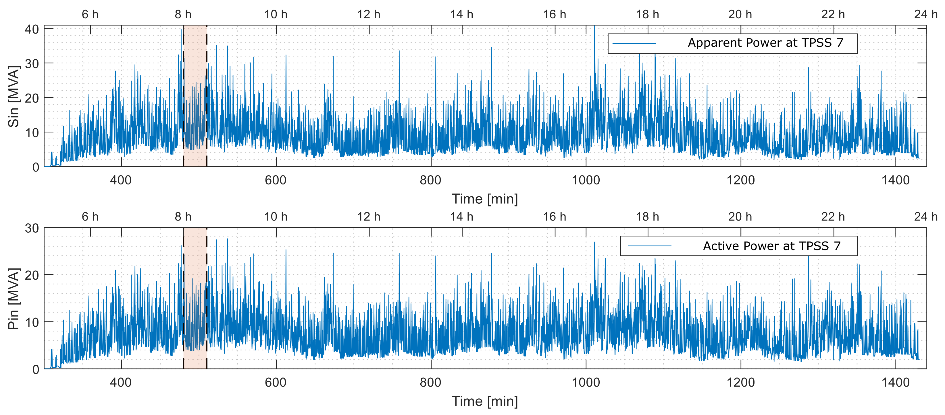
4.1. Substation #7 with Conventional Feeding in Normal Operation

The highly variable apparent power, S in , and active power, P in , absorbed by substation #7 are shown in Figure 6.
As mentioned, without any compensation the unbalanced power gives origin to a negative sequence component of the three-phase voltage at the PCC. For a connection to a three-phase 63 kV voltage level the short circuit power at substation #7 is S SC 3 ϕ = 800 MVA. Accordingly, the corresponding V UF is given (in percentage) in Figure 7.
The V UF profile ranges from zero to near 5%. While important, because it indicates that V UF exceeds 1%, this information is not sufficient either for calculating the effective V UF factor that matters for standards fulfilling or for conformity assessment of quality of service agreements. Usually, larger time windows and averaging factors are used to establish the effective value for V UF [30]. An additional illustrative information is obtained with the plots of the histograms of all substations in terms of the equivalent voltage unbalance factor, where it is used the dataset of timestamped measurements for each TPSS power consumption, sampled at one-second for around 19 h (from 05:00 to 24:00). In Figure 8 is shown this plot and it should be pointed out that the short circuit power is different for each substation.
The seven substations constituting the railway line have different V UF profiles, with substations #3, #4 and #5 having the best interface while substations #1, #6 and #7 are more loaded. Large unbalance factors with high number of occurrences will demand for corrective measures in order to reduce this power quality issue.
In above Figure 8, it is shown the simulated instantaneous apparent and active power. The highlighted window represents 30 min of time. The power factor parameter will be represented in the next two figures below, Figure 9a,b, for the time period considered (from 480 min to 510 min).
Figure 9a represents the single phase power factor in the TPSS 7, using the apparent and active power represented in Figure 6 to calculate their value. In the same Figure 9a is also represented the power factor in the electric grid without any compensation of the unbalanced three-phase current. The difference in the power factor in the electric grid is due to the assumed definition of power factor for unbalanced loads in the electric grid.
Figure 9b shows the power factor in three-phase grid for three different scenarios: (i) Without any compensation; (ii) balance of three-phase load current (the PF is still below one); and (iii) load balance and power factor compensation (unitary power factor is obtained). It is seen that compensation of the negative sequence component of the load current increases the three-phase grid power factor to a value equal to the single-phase load one.
As referred before, we use a definition of power factor for the unbalanced load which includes the definition of apparent power suggested by Buchholz [35]. If we do not use the mentioned approach for grid power factor, but use the IEEE 1459 approach to calculate the power factor, without any compensation we get the power factor profile in Figure 10.
As stated above, the other electric grid parameter analyzed in these results is the three-phase power losses, calculated according to the equivalent circuit in Figure 1. The total power losses in the three-phase grid under different scenarios of load current compensation is represented in Figure 11 and Figure 12, at the point of common coupling of substation #7.
Figure 11 shows the two different scenarios in the point of common coupling: (i) Total losses in three-phase grid without any compensation of the load current (y-axis on the left side); (ii) total losses in three-phase grid with the balance of the three-phase current (y-axis on the left side).
The right y-axis of Figure 10 illustrates the percentage of the power loss decrease after load balancing compared to the initial power losses before load balancing, defined by the expression in (18):
P Δ Loss = P LossB P Loss
This type of compensation results in a constant reduction of the power losses of 50%. The even distribution of the apparent power in the three phases implies a reduction of the r.m.s. value of the current in two phases and an increase in the third one; globally, a significant reduction in the losses is obtained. Figure 12 represents a scenario similar to the one in Figure 11 when full compensation is considered—load balancing and power factor correction.
The right y-axis of Figure 12 represents the percentage of the power losses decrease compared to the initial power losses after load balancing and power factor correction as defined in (19):
P Δ Loss = P LossPF P Loss
Using the results from previous figures to represent the two parameters, power factor and power losses, we can point out some conclusions:
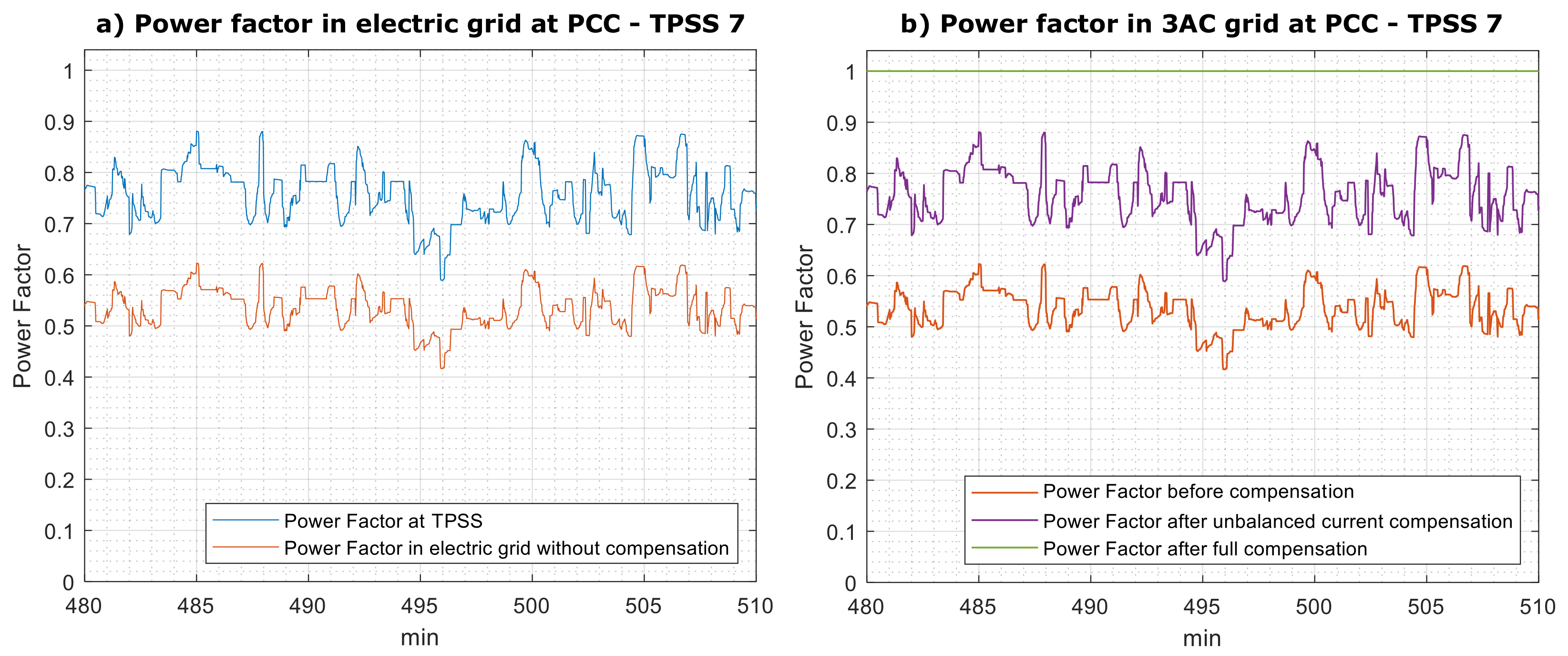
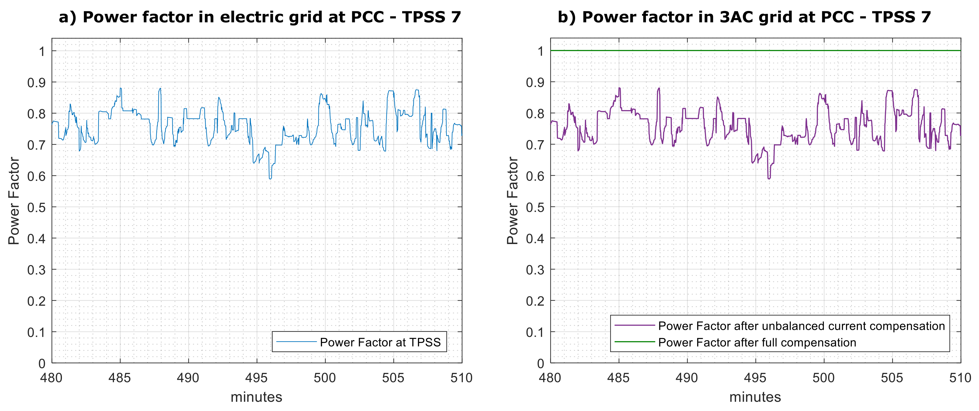
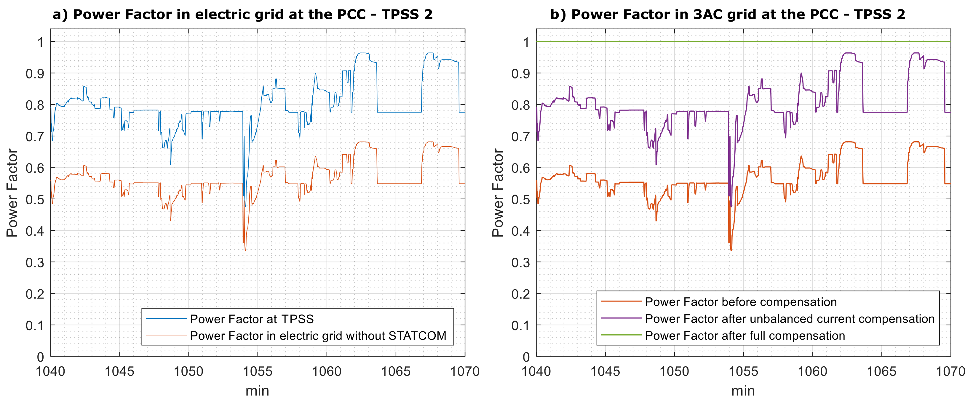
  • In the scenario without compensation of the unbalanced current, the power factor in the three-phase grid has a reduction of 1 / 2 compared with the single phase power factor at the TPSS (Figure 9a).
  • With the compensation of the negative sequence of the unbalanced three-phase current, the power factor in three-phase grid increases by a factor of 2 becoming equal to the load power factor (Figure 9b). Additionally, if reactive power compensation is set, then the grid power factor becomes unitary.
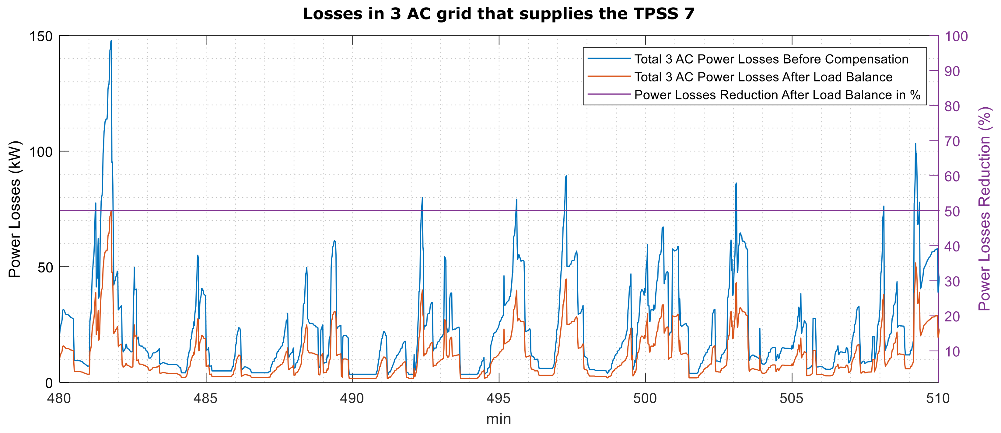
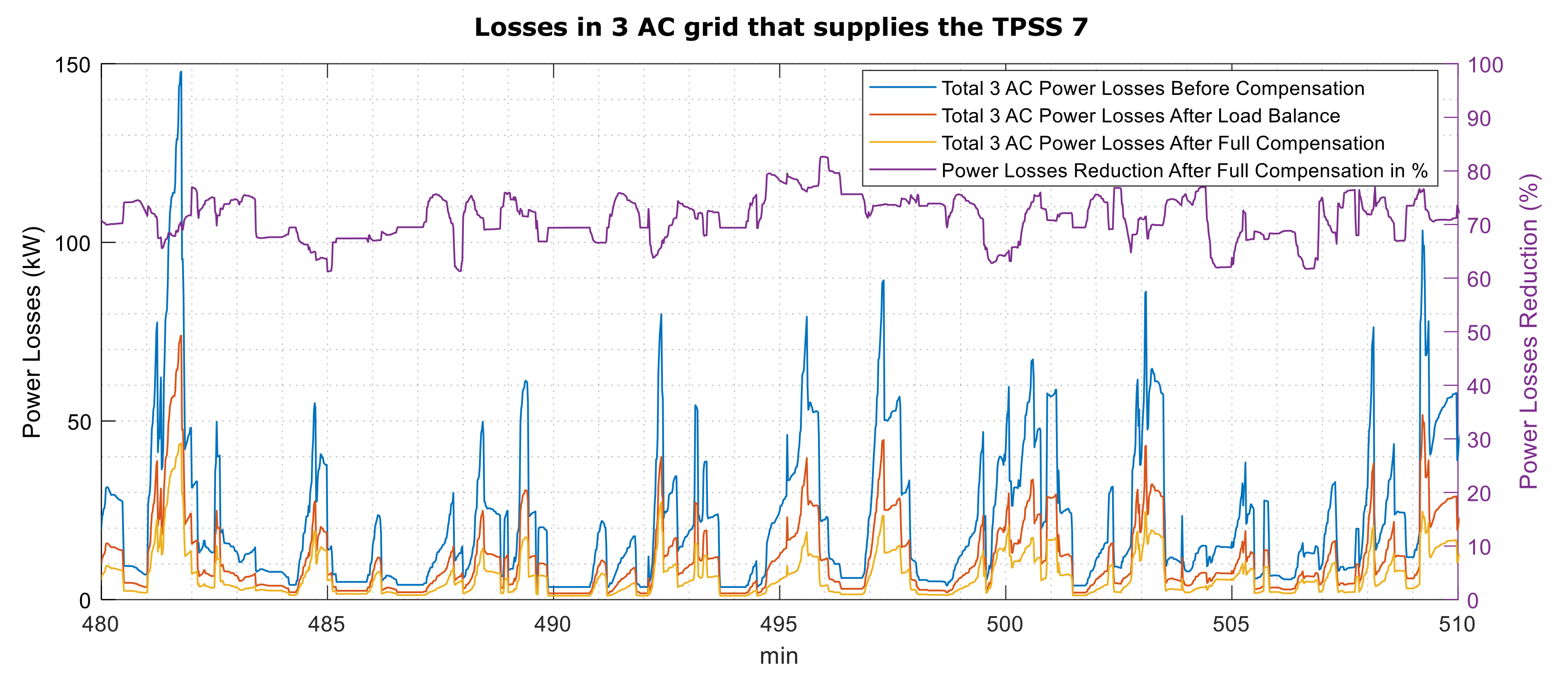
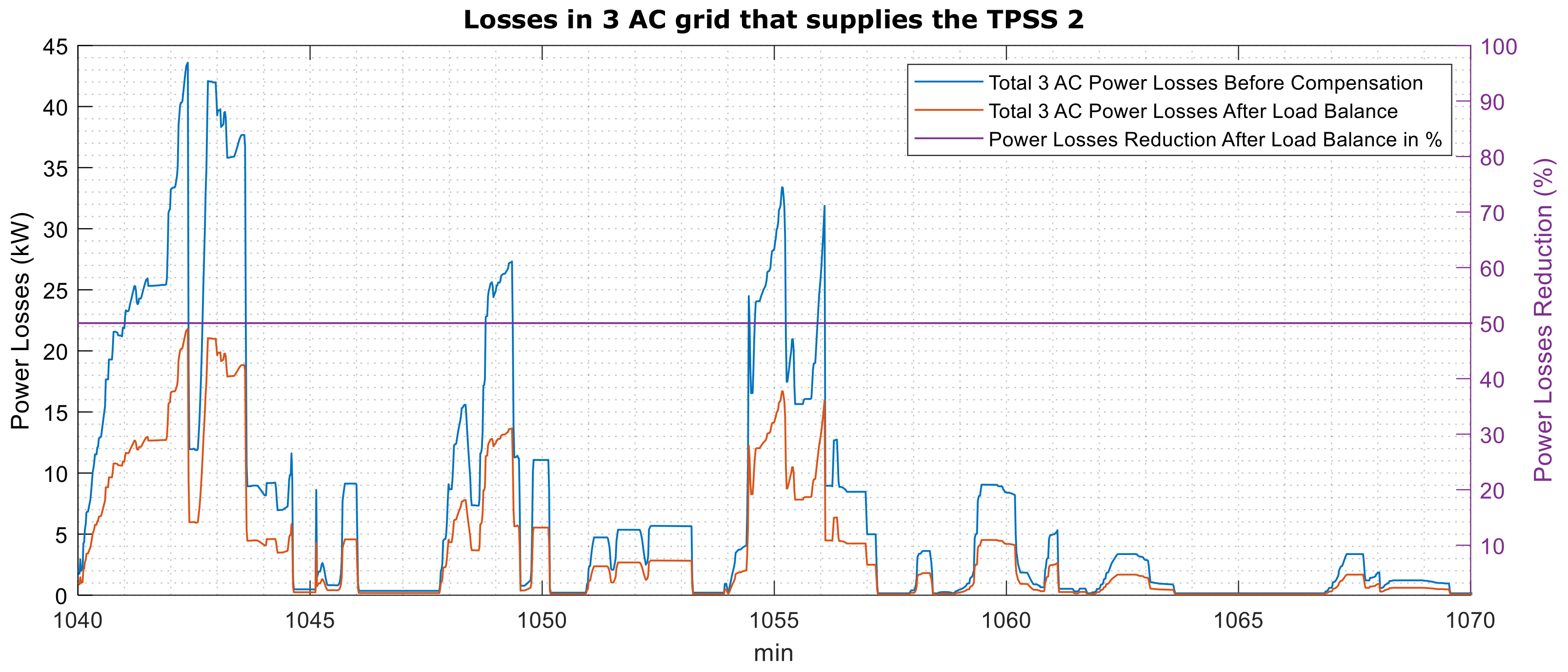
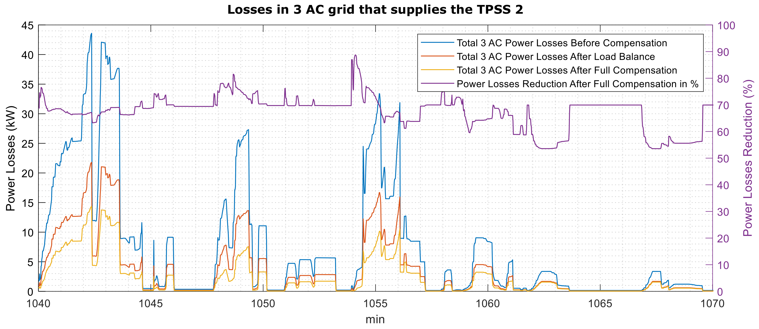
  • Regarding power losses, the compensation of current’s negative sequence component has a consequence of losses decreasing around 50%. This losses’ decrease can be more noticeable by compensating to a unitary power factor in the three-phase grid, as shown in Figure 12.

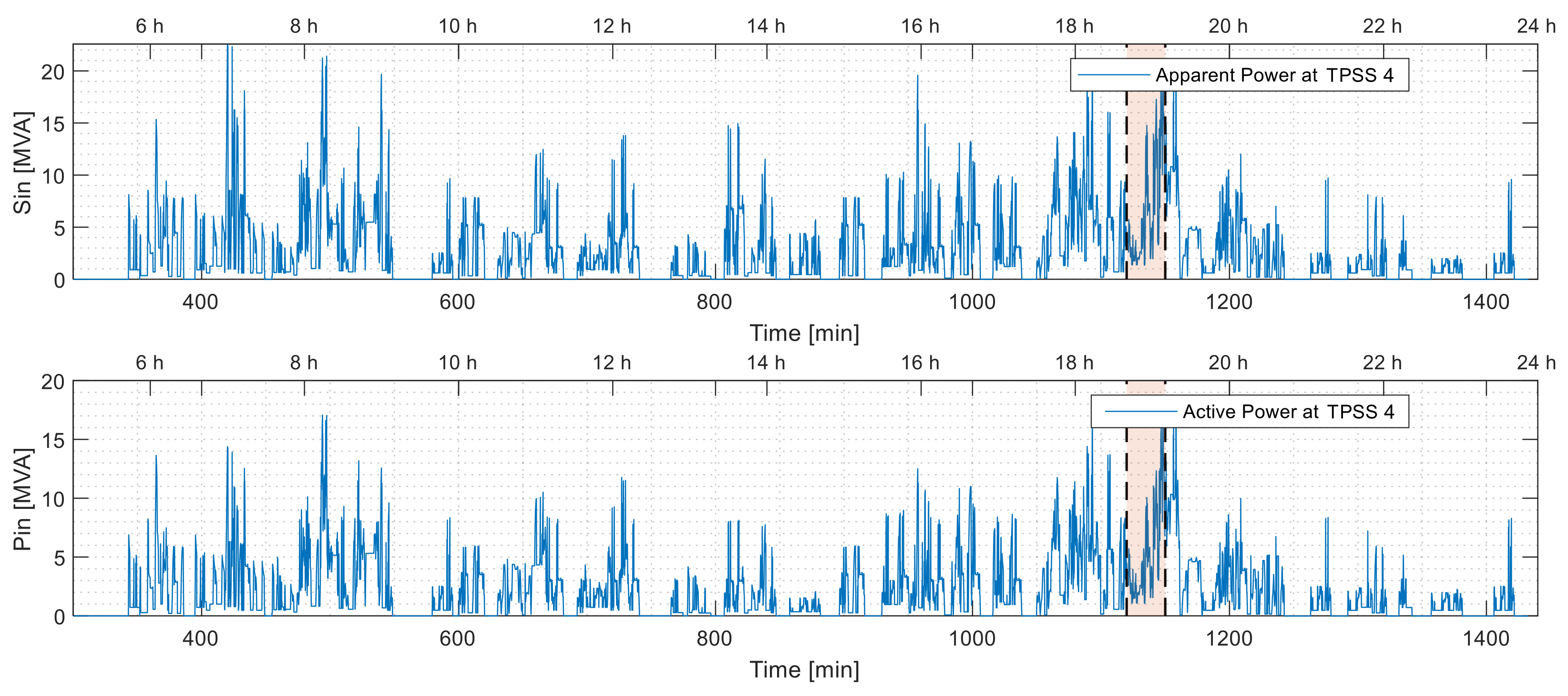
4.2. Substation #4 in Degraded Mode

To analyze some results from a degraded scenario, substation #5 is selected to be placed out of service (OOS) in the simulated scenario, as illustrated in Figure 13. In this degraded mode, the adjacent substations #4 and #6 give the power support in case of a failure scenario (or out of service).
The same procedure employed before is used to analyze the power factor and losses in TPSS 4 towards the evaluation of this OOS scenario. The consumed apparent power, S i n , and active power, P i n , during all analyzed interval are given in Figure 14.
In this scenario, TPSS 5 is out of service. When TPSS 5 is in failure mode during a period of time, the adjacent substations will handle the out of service period of TPSS 5. We selected the time period between 18:40 and 19:10 (from minute 1120 until minute 1150) to analyze the power factor (in Figure 15) and the power losses (in Figure 16 and Figure 17) in the three-phase grid at the point of common coupling.
Regarding power factor behaviour, similar conclusions as the ones obtained from Figure 9 can be verified. In the three-phase grid the power factor increases if the compensation of the negative sequence component is made by the Balancer; it increases to near one if the full compensation is selected.
The same applies to losses in the three-phase grid: Full compensation (Figure 17) obtains the highest reduction in the grid losses.
Using the results from previous figures to represent the power factor and power losses, we have some conclusions:
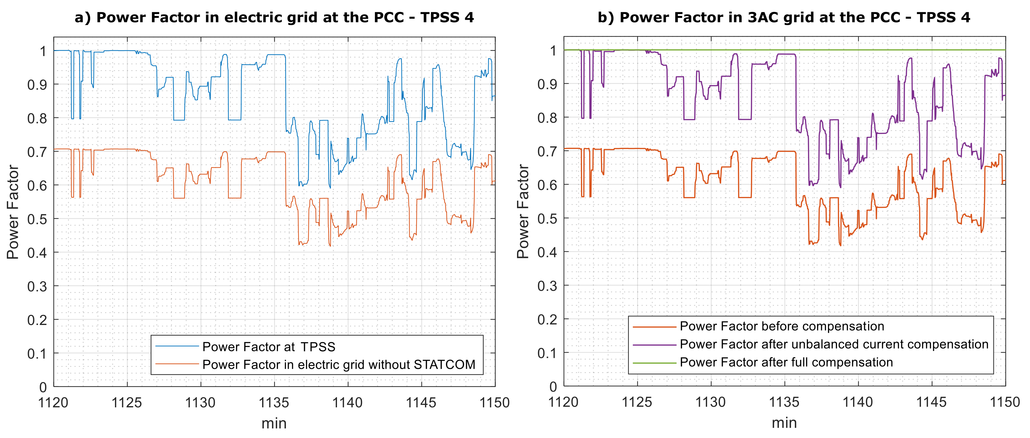
  • Without any compensation of the unbalanced load current, the power factor in the three-phase grid has a reduction of 1 / 2 compared with the single-phase power factor at the TPSS (Figure 15a).
  • With the compensation of the negative sequence of the unbalanced three-phase current, the power factor in three-phase grid increases by a factor of 2 becoming equal to the load power factor. Additionally, if reactive power compensation is used, then the grid power factor becomes unitary (Figure 15b).
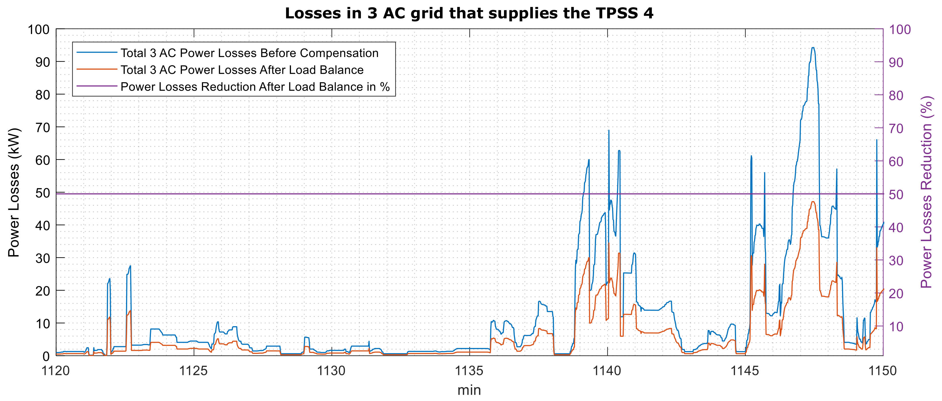
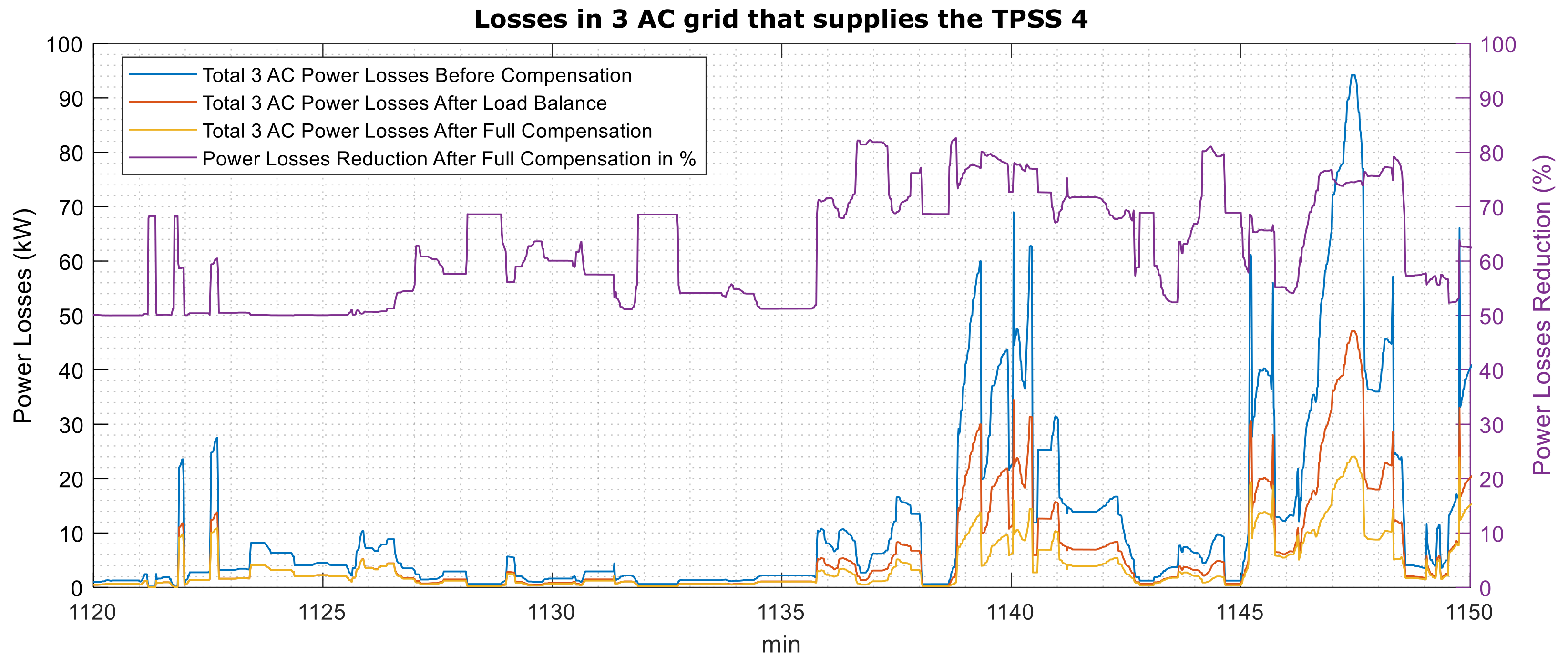
  • Regarding power losses, the compensation of the current’s negative sequence has a consequence of losses decreasing around 50%. This losses’ decrease can be more noticeable by compensating the power factor in the three-phase grid to one, as shown in Figure 17.

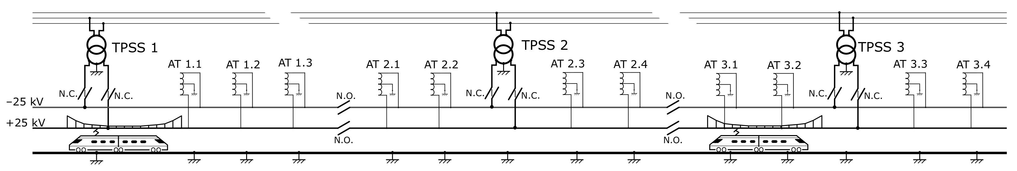
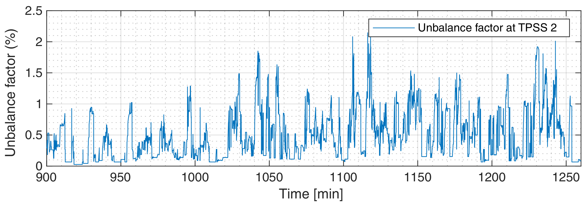
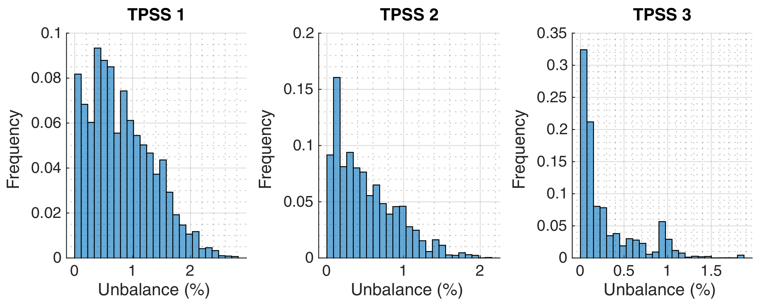
5. Case Study #2: Three Substations

The other line studied in this work is constituted by three substations having a 2 × 25 kV electrification scheme, illustrated in Figure 18.
Since the global results obtained are quite similar to the ones presented for case study #1, it is only presented the results when operating in normal mode and for one substation.

Substation #2 in Normal Operation

The quasi-instantaneous apparent power, S in , and the active power, P in , consumption of a six hours timetable (between 15:00 and 21:00) for substation #2 are shown in Figure 19.
For a connection to a three-phase 220 kV voltage level the short circuit power at substation #2 is S SC 3 ϕ = 1000 MVA. Accordingly, the corresponding V UF is given (in percentage) in Figure 20.
The V UF profile ranges from zero to around 2%. As in case study #1, the occurrence of very different levels for V UF can be better visualized with a histogram of the results, shown in Figure 21 for the three substations, although they are not enough for a complete characterization of this parameter.
Substation #3 appears to have a better interface to the electric grid in terms of power quality while substations #1 and #2 might require further attention in terms of monitoring.
The time period selected to analyze the power factor and the power losses in the three-phase grid is from 17:20 to 17:50 (1040 min–1070 min). The power factor evaluation is shown in Figure 22.
Regarding power factor behaviour, similar conclusions as the ones obtained from Figure 9 and Figure 15 are obtained. In the three-phase grid the power factor increases if the compensation of the negative sequence component is made by the Balancer; it increases to near one if the full compensation is made.
In relation to power losses the results for this analysis are shown in Figure 23 and Figure 24 for the two possible compensation modes: Current balancing only and full compensation mode.
Similarly to the power factor and also for the power losses, the conclusions are similar to the ones obtained regarding case study #1. In both compensation modes there is an important reduction of the power losses when comparing with the system operating without any compensation.
The inclusion of the Balancer in the 2 × 25 kV electrification scheme could be justified by similar reasons: The distances between substations are longer and the power requirements are usually also higher than in 1 × 25 kV. Thus, the unbalance factor, the power factor and the equivalent power losses in the three-phase grid have the same or higher importance.

6. Conclusions

The power quality issues associated with the unbalanced current in the three-phase power grid caused by the single-phase railway electrification structure were addressed in this paper. An electronic balancer can reduce/eliminate the negative sequence component of the three-phase current, contributing to strongly reduce the voltage unbalance factor, to increase the power factor value and to lower the power losses. The methodology to validate the impact of this electronic balancer was proposed in this paper, using a database of two different railway lines: One with 1 × 25 kV with seven substations and the second with a 2 × 25 kV with three substations.
For each dataset, first it was evaluated a baseline scenario without compensation, then it was compensated the negative sequence component of the current towards a balanced power supply at the PCC, and finally the reactive power is minimized to achieve a unitary power factor.
Analyzing the global results presented in this study, it can be concluded that there are no differences in the system behavior, in normal mode or degraded mode, with 1 × 25 kV or 2 × 25 kV supply, if the compensation mode is the same. A balanced three-phase current does not originate any voltage unbalance factor and relevant gains are obtained either in three-phase power factor or grid power losses when the negative sequence component of the load current is compensated. Additionally, but not so relevant, further improvements are obtained in the last two parameters if the load power factor is also compensated.
Globally, the compensation of the negative sequence component of the load current in the three-phase grid brings important benefits to the power quality of the electrification system. The improvement in the power factor and the losses reduction are the most relevant, with the results and findings presented in this paper supporting the advantages of using an electronic balancer.

Author Contributions

Conceptualization, A.P.M., P.R., M.H. and V.A.M.; Funding acquisition, A.P.M. and M.H.; Investigation, A.P.M. and P.R.; Methodology, A.P.M. and P.R.; Software, A.P.M. and P.R.; Writing–original draft, A.P.M. and V.A.M.; Writing–review & editing, A.P.M. and V.A.M. All authors have read and agreed to the published version of the manuscript.

Funding

In2Stempo project has received funding from the Shift2Rail Joint Undertaking under the European Union’s Horizon 2020 grant agreement no 777515. This work was supported by UIDB/00147/2020–SYSTEC-Research Centre for Systems and Technologies, funded by national funds through the FCT/MCTES (PIDDAC).

Institutional Review Board Statement

Not applicable.

Informed Consent Statement

Not applicable.

Data Availability Statement

Due to confidentiality restrictions, no data is made publicly available from this study.

Conflicts of Interest

The authors declare no conflict of interest.

Abbreviations

The following abbreviations are used in this manuscript:
DFIGDoubly Fed Induction Generators
EHVExtra-High Voltage
FACTSFlexible AC Transmission Systems
FBDFryze Buchholz Depenbrock
HVHigh Voltage
HSRHigh Speed Railway
IEEEInstitute of Electrical and Electronics Engineers
IN2STEMPOInnovative Solutions in Future Stations, Energy Metering and Power Supply
JUJoint Undertaking
NSCNegative Sequence Component
OOSOut of Service
PCCPoint of Common Coupling
PFPower Factor
PLLPhase-Locked Loop
PRProportional plus Resonant
PSCPositive Sequence Component
RPCRail Power Conditioner
S2RShift2Rail
SFCStatic Frequency Converter
STATCOMStatic Synchronous Compensator
SVCStatic Var Compensator
TPSSTraction Power Substations
TSO/DSOTransmission System Operator/Distribution System Operator
ZSCZero Sequence Component

References

  1. Shift2Rail. Multi-Annual Action Plan; Publications Office of the European Union: Luxembourg, 2019. [Google Scholar] [CrossRef]
  2. European Comission. Innovative Solutions in Future Stations, Energy Metering and Power Supply. 2019. Available online: https://cordis.europa.eu/project/id/777515 (accessed on 10 October 2021).
  3. ABB. SVCs for Load Balancing and Trackside Voltage Control; Technical Report; ABB: Västerås, Sweden, 2010. [Google Scholar]
  4. Lee, S.Y.; Wu, C.J.; Chang, W.N. A compact control algorithm for reactive power compensation and load balancing with static Var compensator. Electr. Power Syst. Res. 2001, 58, 63–70. [Google Scholar] [CrossRef]
  5. Sainz, L.; Caro, E.; Riera, S. Characterization of Harmonic Resonances in the Presence of the Steinmetz Circuit in Power Systems. In Power Quality Harmonics Analysis and Real Measurements Data; Romero, G., Ed.; IntechOpen: London, UK, 2011; Chapter 7. [Google Scholar] [CrossRef] [Green Version]
  6. Konishi, S.; Baba, K.; Daiguji, M. Var Compensators. Fuji Electr. Rev. 2002, 48, 37–45. [Google Scholar]
  7. Grunbaum, R.; Halvarsson, P.; Thorvaldsson, B. Knowing the FACTS. ABB Rev. 2010, 2, 35–41. [Google Scholar]
  8. Gruber, R.; O’Brien, D. Use of Modular Multilevel Converter (MMC) Technology in Rail Electrification. In Proceedings of the AusRAIL 2014, Making Making Innovation Work, Perth, Australia, 11–12 November 2014. [Google Scholar]
  9. Hayashiya, H.; Kondo, K. Recent trends in power electronics applications as solutions in electric railways. IEEJ Trans. Electr. Electron. Eng. 2020, 15, 632–645. [Google Scholar] [CrossRef]
  10. Hu, S.; Wu, B.; Rehtanz, C.; Zhang, Z.; Chen, Y.; Zhou, G.; Li, Y.; Luo, L.; Cao, Y.; Xie, B.; et al. A New Integrated Hybrid Power Quality Control System for Electrical Railway. IEEE Trans. Ind. Electron. 2015, 62, 6222–6232. [Google Scholar] [CrossRef]
  11. Tokiwa, A.; Yamada, H.; Tanaka, T.; Watanabe, M.; Shirai, M.; Teranishi, Y. New Hybrid Static VAR Compensator with Series Active Filter. Energies 2017, 10, 1617. [Google Scholar] [CrossRef]
  12. Abrahamsson, L.; Schütte, T.; Östlund, S. Use of converters for feeding of AC railways for all frequencies. Energy Sustain. Dev. 2012, 16, 368–378. [Google Scholar] [CrossRef] [Green Version]
  13. Krastev, I.; Tricoli, P.; Hillmansen, S.; Chen, M. Future of Electric Railways: Advanced Electrification Systems with Static Converters for ac Railways. IEEE Electrif. Mag. 2016, 4, 6–14. [Google Scholar] [CrossRef]
  14. Sun, Z.; Jiang, X.; Zhu, D.; Zhang, G. A Novel Active Power Quality Compensator Topology for Electrified Railway. IEEE Trans. Power Electron. 2004, 19, 1036–1042. [Google Scholar] [CrossRef]
  15. Chen, M.; Li, Q.; Roberts, C.; Hillmansen, S.; Tricoli, P.; Zhao, N.; Krastev, I. Modelling and performance analysis of advanced combined co-phase traction power supply system in electrified railway. IET Gener. Transm. Distrib. 2016, 10, 906–916. [Google Scholar] [CrossRef]
  16. Uzuka, T.; Ikedo, S.; Ueda, K. A static voltage fluctuation compensator for AC electric railway. In Proceedings of the 2004 IEEE 35th Annual Power Electronics Specialists Conference (IEEE Cat. No.04CH37551), Aachen, Germany, 20–25 June 2004. [Google Scholar] [CrossRef]
  17. Tanta, M.; Pinto, J.G.; Monteiro, V.; Martins, A.P.; Carvalho, A.S.; Afonso, J.L. Topologies and Operation Modes of Rail Power Conditioners in AC Traction Grids: Review and Comprehensive Comparison. Energies 2020, 13, 2151. [Google Scholar] [CrossRef]
  18. Paszkier, B.; Zouiti, M.; Javerzac, J.L.; Perret, J.P.; Courtois, C. VSC based imbalance compensator for railway substations. In Proceedings of the 41st Session of the International Conference on Large High Voltage Electric Systems (CIGRE), Paris, France, 27 August 27–1 September 2006. [Google Scholar]
  19. Tanta, M.; Cunha, J.; Barros, L.A.M.; Monteiro, V.; Pinto, J.G.O.; Martins, A.P.; Afonso, J.L. Experimental Validation of a Reduced-Scale Rail Power Conditioner Based on Modular Multilevel Converter for AC Railway Power Grids. Energies 2021, 14, 484. [Google Scholar] [CrossRef]
  20. Bueno, A.; Aller, J.M.; Restrepo, J.A.; Harley, R.; Habetler, T.G. Harmonic and Unbalance Compensation Based on Direct Power Control for Electric Railway Systems. IEEE Trans. Power Electron. 2013, 28, 5823–5831. [Google Scholar] [CrossRef]
  21. He, Z.; Zheng, Z.; Hu, H. Power quality in high-speed railway systems. Int. J. Rail Transp. 2016, 4, 71–97. [Google Scholar] [CrossRef] [Green Version]
  22. Kaleybar, H.J.; Brenna, M.; Foiadelli, F.; Fazel, S.S.; Zaninelli, D. Power Quality Phenomena in Electric Railway Power Supply Systems: An Exhaustive Framework and Classification. Energies 2020, 13, 6662. [Google Scholar] [CrossRef]
  23. Oghorada, O.J.K.; Zhang, L. Unbalanced and Reactive Load Compensation Using MMCC-Based SATCOMs With Third-Harmonic Injection. IEEE Trans. Ind. Electron. 2019, 66, 2891–2902. [Google Scholar] [CrossRef] [Green Version]
  24. Yuan, J.; Xiao, F.; Zhang, C.; Chen, Y.; Ni, Z.; Zhong, Y. Collaborative unbalance compensation method for high-speed railway traction power supply system considering energy feedback. IET Power Electron. 2019, 12, 129–137. [Google Scholar] [CrossRef]
  25. Tareen, W.; Aamir, M.; Mekhilef, S.; Nakaoka, M.; Seyedmahmoudian, M.; Horan, B.; Memon, M.; Baig, N. Mitigation of Power Quality Issues Due to High Penetration of Renewable Energy Sources in Electric Grid Systems Using Three-Phase APF/STATCOM Technologies: A Review. Energies 2018, 11, 1491. [Google Scholar] [CrossRef] [Green Version]
  26. Chen, Y.; Chen, M.; Tian, Z.; Liu, Y.; Hillmansen, S. VU limit pre-assessment for high-speed railway considering a grid connection scheme. IET Gener. Transm. Distrib. 2019, 13, 1121–1131. [Google Scholar] [CrossRef]
  27. Chen, Y.; Chen, M.; Tian, Z.; Liu, Y. Voltage Unbalance Management for High-Speed Railway Considering the Impact of Large-Scale DFIG-Based Wind Farm. IEEE Trans. Power Deliv. 2020, 35, 1667–1677. [Google Scholar] [CrossRef]
  28. Xiao, D.; Minwu, C.; Yinyu, C. Negative Sequence Current and Reactive Power Comprehensive Compensation for Freight Railway Considering the Impact of DFIGs. CPSS Trans. Power Electron. Appl. 2021, 6, 235–241. [Google Scholar] [CrossRef]
  29. IEC. Electromagnetic Compatibility (EMC)-Part 3-13: Limits-Assessment of Emission Limits for the Connection of Unbalanced Installations to MV, HV and EHV Power Systems; IEC/TR 61000-3-13; IEC: Geneva, Switzerland, 2008. [Google Scholar]
  30. IEC. Electromagnetic compatibility (EMC)-Part 4-30: Testing and Measurement Techniques-Power Quality Measurement Methods; IEC/TR 61000-4-30; IEC: Geneva, Switzerland, 2008. [Google Scholar]
  31. Paap, G.C. Symmetrical components in the time domain and their application to power network calculations. IEEE Trans. Power Syst. 2000, 15, 522–528. [Google Scholar] [CrossRef]
  32. Chen, T.H. Criteria to estimate the voltage unbalances due to high-speed railway demands. IEEE Trans. Power Syst. 1994, 9, 1672–1678. [Google Scholar] [CrossRef]
  33. Plantive, E.; Courtois, C.; Javerzac, J.L.; Poirrier, J.P. Application of a 20 MVA STATCOM for voltage balancing and power active filtering of a 25 kV AC single-phase railway substation connected to the 90 kV grid in France. In Proceedings of the 38th Session of the International Conference on Large High Voltage Electric Systems (CIGRE), Paris, France, 27 August–1 September 2000. [Google Scholar]
  34. Simões, M.G.; Harirchi, F.; Babakmehr, M. Survey on time-domain power theories and their applications for renewable energy integration in smart-grids. IET Smart Grid 2019, 2, 491–503. [Google Scholar] [CrossRef]
  35. Depenbrock, M. The FBD-method, a generally applicable tool for analyzing power relations. IEEE Trans. Power Syst. 1993, 8, 381–387. [Google Scholar] [CrossRef]
  36. Willems, J.L. IEEE Standard 1459. IEEE Standard Definitions for the Measurement of Electric Power Quantities Under Sinusoidal, Nonsinusoidal, Balanced, or Unbalanced Conditions. In Proceedings of the 2010 IEEE International Workshop on Applied Measurements for Power Systems, Aachen, Germany, 22–24 September 2010. [Google Scholar] [CrossRef] [Green Version]
  37. Laka, A.; Cross, A.; Barrena, J.A.; Chivite-Zabalza, J.; Rodriguez, M.A. VSC topology comparison for STATCOM application under unbalanced conditions. In Proceedings of the 2013 15th European Conference on Power Electronics and Applications (EPE), Lille, France, 2–6 September 2013. [Google Scholar] [CrossRef] [Green Version]
  38. Hochgraf, C.; Lasseter, R.H. Statcom controls for operation with unbalanced voltages. IEEE Trans. Power Deliv. 1998, 13, 538–544. [Google Scholar] [CrossRef] [Green Version]
  39. Martins, A.P.; Morais, V.A.; Ramos, C.J. Analysis of the STATCOM/Balancer Robustness in Railway Applications. In Proceedings of the 2020 IEEE 14th International Conference on Compatibility, Power Electronics and Power Engineering (CPE-POWERENG), Setubal, Portugal, 8–10 July 2020. [Google Scholar] [CrossRef]
  40. Akagi, H.; Watanabe, E.H.; Aredes, M. Instantaneous Power Theory and Applications to Power Conditioning, 2nd ed.; John Wiley & Sons, Inc.: Hoboken, NJ, USA, 2017. [Google Scholar] [CrossRef]
  41. Kazmierkowski, M.; Malesani, L. Current control techniques for three-phase voltage-source PWM converters: A survey. IEEE Trans. Ind. Electron. 1998, 45, 691–703. [Google Scholar] [CrossRef]
  42. Zmood, D.; Holmes, D. Stationary frame current regulation of PWM inverters with zero steady-state error. IEEE Trans. Power Electron. 2003, 18, 814–822. [Google Scholar] [CrossRef]
Figure 1. Electronic Balancer for compensation of the single-phase connection of a traction substation to a HV/EHV grid.
Electricity 02 00032 g001
Figure 2. Examples of possible architecture for the V-V based TPSS (a) and possible solution for power structure of the electronic balancer using modular multilevel converter (b).
Electricity 02 00032 g002
Figure 3. Control diagram of the Balancer system.
Electricity 02 00032 g003
Figure 4. Simplified diagram of case study #1 substations.
Electricity 02 00032 g004
Figure 5. The range of apparent power in percentages per number of occurrences.
Electricity 02 00032 g005
Figure 6. Apparent and active power consumed at substation #7.
Electricity 02 00032 g006
Figure 7. Voltage unbalance factor profile at the PCC corresponding to substation #7.
Electricity 02 00032 g007
Figure 8. Voltage unbalance factor histograms corresponding to TPSS 1 to TPSS 7.
Electricity 02 00032 g008
Figure 9. Power factor at substation #7 with and without compensation: (a) single-phase; (b) three-phase.
Electricity 02 00032 g009
Figure 10. Power factor at substation #7: (a) single-phase; (b) three-phase, in the three-phase grid side, with different types of compensation.
Electricity 02 00032 g010
Figure 11. Power losses in the three-phase grid supplying substation #7.
Electricity 02 00032 g011
Figure 12. Power losses in the three-phase grid supplying substation #7 with different compensation options.
Electricity 02 00032 g012
Figure 13. Connections of substations #4, #5 and #6 in a degraded mode.
Electricity 02 00032 g013
Figure 14. Apparent and active power consumption in TPSS 4 when TPSS 5 is out of service.
Electricity 02 00032 g014
Figure 15. Power factor in the three-phase grid when TPSS 4 is operating in degraded mode: (a) without Balancer compensation; (b) with Balancer compensation.
Electricity 02 00032 g015
Figure 16. Losses in the three-phase grid supplying TPSS 4 when TPSS 5 is out of service.
Electricity 02 00032 g016
Figure 17. Power losses and losses reduction in the three-phase grid supplying the TPSS 4 with different compensation options.
Electricity 02 00032 g017
Figure 18. Single-line diagram of case study #2, a 2 × 25 kV line.
Electricity 02 00032 g018
Figure 19. Apparent and active power consumption at substation #2 in normal mode.
Electricity 02 00032 g019
Figure 20. Voltage unbalance factor profile at TPSS 2, in case study #2.
Electricity 02 00032 g020
Figure 21. Histogram of V UF for the three substations constituting the line in case study #2.
Electricity 02 00032 g021
Figure 22. Power factor in the three-phase grid when TPSS 2 is operating in normal mode: (a) without Balancer compensation; (b) with Balancer compensation.
Electricity 02 00032 g022
Figure 23. Losses (left axis) and losses reduction (right axis) in the three-phase grid supplying substation #2 in normal mode without and with load balancing.
Electricity 02 00032 g023
Figure 24. Losses (left axis) and losses reduction (right axis) in the three-phase grid supplying substation #2 with different compensation options.
Electricity 02 00032 g024
Publisher’s Note: MDPI stays neutral with regard to jurisdictional claims in published maps and institutional affiliations.

